Using cTWAS - Multigroup Branch
wesleycrouse
2023-09-11
Last updated: 2023-10-21
Checks: 6 1
Knit directory: ctwas_applied/
This reproducible R Markdown analysis was created with workflowr (version 1.7.0). The Checks tab describes the reproducibility checks that were applied when the results were created. The Past versions tab lists the development history.
The R Markdown file has unstaged changes. To know which version of
the R Markdown file created these results, you’ll want to first commit
it to the Git repo. If you’re still working on the analysis, you can
ignore this warning. When you’re finished, you can run
wflow_publish to commit the R Markdown file and build the
HTML.
Great job! The global environment was empty. Objects defined in the global environment can affect the analysis in your R Markdown file in unknown ways. For reproduciblity it’s best to always run the code in an empty environment.
The command set.seed(20210726) was run prior to running
the code in the R Markdown file. Setting a seed ensures that any results
that rely on randomness, e.g. subsampling or permutations, are
reproducible.
Great job! Recording the operating system, R version, and package versions is critical for reproducibility.
Nice! There were no cached chunks for this analysis, so you can be confident that you successfully produced the results during this run.
Great job! Using relative paths to the files within your workflowr project makes it easier to run your code on other machines.
Great! You are using Git for version control. Tracking code development and connecting the code version to the results is critical for reproducibility.
The results in this page were generated with repository version 29b99ed. See the Past versions tab to see a history of the changes made to the R Markdown and HTML files.
Note that you need to be careful to ensure that all relevant files for
the analysis have been committed to Git prior to generating the results
(you can use wflow_publish or
wflow_git_commit). workflowr only checks the R Markdown
file, but you know if there are other scripts or data files that it
depends on. Below is the status of the Git repository when the results
were generated:
Untracked files:
    Untracked:  gwas.RData
    Untracked:  ld_R_info.RData
    Untracked:  z_snp_pos_ebi-a-GCST004131.RData
    Untracked:  z_snp_pos_ebi-a-GCST004132.RData
    Untracked:  z_snp_pos_ebi-a-GCST004133.RData
    Untracked:  z_snp_pos_scz-2018.RData
    Untracked:  z_snp_pos_ukb-a-360.RData
    Untracked:  z_snp_pos_ukb-d-30780_irnt.RData

Unstaged changes:
    Modified:   analysis/transition_multigroup.Rmd
Note that any generated files, e.g. HTML, png, CSS, etc., are not included in this status report because it is ok for generated content to have uncommitted changes.
These are the previous versions of the repository in which changes were
made to the R Markdown (analysis/transition_multigroup.Rmd)
and HTML (docs/transition_multigroup.html) files. If you’ve
configured a remote Git repository (see ?wflow_git_remote),
click on the hyperlinks in the table below to view the files as they
were in that past version.
| File | Version | Author | Date | Message |
|---|---|---|---|---|
| Rmd | 29b99ed | wesleycrouse | 2023-09-28 | adding preharmonization |
| html | 29b99ed | wesleycrouse | 2023-09-28 | adding preharmonization |
| Rmd | 3384c1b | wesleycrouse | 2023-09-14 | fixing typo |
| html | 3384c1b | wesleycrouse | 2023-09-14 | fixing typo |
| Rmd | 7edeea5 | wesleycrouse | 2023-09-14 | updating user guide for new harmonization option |
| html | 7edeea5 | wesleycrouse | 2023-09-14 | updating user guide for new harmonization option |
| Rmd | 3147f25 | wesleycrouse | 2023-09-12 | adding user guide for multigroup branch |
| html | 3147f25 | wesleycrouse | 2023-09-12 | adding user guide for multigroup branch |
| Rmd | e3b2903 | wesleycrouse | 2023-08-31 | adding transition documents |
Overview
This document is a user guide for multigroup branch of
the cTWAS R package, which is under development. It details how to use
to use the summary statistics version of cTWAS with multiple groups of
prediciton models. This can be used to jointly analyze gene expression
from multiple tissues, or to jointly analyze prediction models from
different types of -omics data (i.e. gene expression and chromatin
accessibility), among other potential uses. This version of cTWAS also
includes several performance improvements and additional options to
divide up the analysis for large jobs. Additional details about cTWAS
are available in the paper. This
document assumes that you have already read the user guide for the
main branch of cTWAS, available here.
Getting started
Start by installing the multigroup branch of cTWAS in R
via GitHub:
remotes::install_github("xinhe-lab/ctwas", ref = "multigroup")Then load the package and set the working directory where you want to perform perform the analysis.
library(ctwas)

#set the working directory interactively
setwd("/project2/mstephens/wcrouse/ctwas_tutorial")

#set the working directory when compiling this document with Knitr
knitr::opts_knit$set(root.dir = "/project2/mstephens/wcrouse/ctwas_tutorial")
Preparing input data
The inputs for the summary statistics version of cTWAS include GWAS summary statistics for variants, prediction models for genes in PredictDB format, and an LD reference.
These inputs should be harmonized prior to analysis (i.e. the reference and alternative alleles for each variant should match across all three data sources). We provide some options for harmonization if the data are not already harmonized. See the section on harmonization for more details.
GWAS z-scores
For this analysis, we will use summary statistics from a GWAS of LDL cholesterol in the UK Biobank. We will download the VCF from the IEU Open GWAS Project. Set the working directory, download the summary statistics, and unzip the file.
dir.create("gwas_summary_stats")

system("wget https://gwas.mrcieu.ac.uk/files/ukb-d-30780_irnt/ukb-d-30780_irnt.vcf.gz -P gwas_summary_stats")
R.utils::gunzip("gwas_summary_stats/ukb-d-30780_irnt.vcf.gz")
Next, we will use the VariantAnnotation package to read the summary statistics. Then, we will compute the z-scores and format the input data. We will also collect the sample size, which will be useful later. We will save this output for convenience.
#read the data
z_snp <- VariantAnnotation::readVcf("gwas_summary_stats/ukb-d-30780_irnt.vcf")
z_snp <- as.data.frame(gwasvcf::vcf_to_tibble(z_snp))

#compute the z-scores
z_snp$Z <- z_snp$ES/z_snp$SE

#collect sample size (most frequent sample size for all variants)
gwas_n <- as.numeric(names(sort(table(z_snp$SS),decreasing=TRUE)[1]))

#subset the columns and format the column names
z_snp <- z_snp[,c("rsid", "ALT", "REF", "Z")]
colnames(z_snp) <- c("id", "A1", "A2", "z")

#drop multiallelic variants (id not unique)
z_snp <- z_snp[!(z_snp$id %in% z_snp$id[duplicated(z_snp$id)]),]

#save the formatted z-scores and GWAS sample size
saveRDS(z_snp, file="gwas_summary_stats/ukb-d-30780_irnt.RDS")
saveRDS(gwas_n, file="gwas_summary_stats/gwas_n.RDS")
After the previous step has run, we can load the data and look at the format. Z_snp is a data frame, and each row is a variant. A1 is the alternate allele, and A2 is the reference allele. The sample size for this GWAS is N=343,621.
z_snp <- readRDS("gwas_summary_stats/ukb-d-30780_irnt.RDS")
gwas_n <- readRDS("gwas_summary_stats/gwas_n.RDS")

head(z_snp)
id A1 A2 z
1 rs530212009 C CA -1.10726803
2 rs12238997 G A -1.05210759
3 rs371890604 C G -1.27724687
4 rs144155419 A G -0.84645309
5 rs189787166 T A -0.05504189
6 rs148120343 C T -1.23068731gwas_n[1] 343621Prediction models
The multigroup version of cTWAS only accepts multiple
sets of prediction models in PredictDB format. A single set of
prediction models can still be specified in FUSION format, as in the
main branch. See the section on converting between FUSION
and PredictDB weights for guidence on using multiple sets of FUSION
weights.
To specify weights in PredictDB format, provide the path to the
.db file. Multiple prediction models can be specified by
providing multiple paths as a vector.
For this analysis, we will use liver and subcutaneous adipose gene
expression models trained on GTEx v8 in the PredictDB format. We will
download both the prediction models (.db) and the
covariances between variants in the prediction models
(.txt.gz). The covariances can optionally be used during
harmonization to recover strand ambiguous variants.
#download the files
system("wget https://zenodo.org/record/3518299/files/mashr_eqtl.tar")

#extract to ./weights folder
system("mkdir weights")
system("tar -xvf mashr_eqtl.tar -C weights")
system("rm mashr_eqtl.tar")
In the paper, we also performed an additional preprocessing step to remove lncRNAs from the prediction models. This can be done using the following code:
library(RSQLite)

#####processing liver weights

#specify the weight to remove lncRNA from
weight <- "weights/eqtl/mashr/mashr_Liver.db"

#read the PredictDB weights
sqlite <- dbDriver("SQLite")
db = dbConnect(sqlite, weight)
query <- function(...) dbGetQuery(db, ...)
weights_table <- query("select * from weights")
extra_table <- query("select * from extra")
dbDisconnect(db)

#subset to protein coding genes only
extra_table <-  extra_table[extra_table$gene_type=="protein_coding",,drop=F]
weights_table <- weights_table[weights_table$gene %in% extra_table$gene,]

#read and subset the covariances
weight_info = read.table(gzfile(paste0(tools::file_path_sans_ext(weight), ".txt.gz")), header = T)
weight_info <- weight_info[weight_info$GENE %in% extra_table$gene,]

#write the .db file and the covariances
dir.create("weights_nolnc", showWarnings=F)

if (!file.exists("weights_nolnc/mashr_Liver_nolnc.db")){
  db <- dbConnect(sqlite, "weights_nolnc/mashr_Liver_nolnc.db")
  dbWriteTable(db, "extra", extra_table)
  dbWriteTable(db, "weights", weights_table)
  dbDisconnect(db)

  weight_info_gz <- gzfile("weights_nolnc/mashr_Liver_nolnc.txt.gz", "w")
  write.table(weight_info, weight_info_gz, sep=" ", quote=F, row.names=F, col.names=T)
  close(weight_info_gz)
}

#####processing adipose weights

#specify the weight to remove lncRNA from
weight <- "weights/eqtl/mashr/mashr_Adipose_Subcutaneous.db"

#read the PredictDB weights
sqlite <- dbDriver("SQLite")
db = dbConnect(sqlite, weight)
query <- function(...) dbGetQuery(db, ...)
weights_table <- query("select * from weights")
extra_table <- query("select * from extra")
dbDisconnect(db)

#subset to protein coding genes only
extra_table <-  extra_table[extra_table$gene_type=="protein_coding",,drop=F]
weights_table <- weights_table[weights_table$gene %in% extra_table$gene,]

#read and subset the covariances
weight_info = read.table(gzfile(paste0(tools::file_path_sans_ext(weight), ".txt.gz")), header = T)
weight_info <- weight_info[weight_info$GENE %in% extra_table$gene,]

#write the .db file and the covariances
dir.create("weights_nolnc", showWarnings=F)

if (!file.exists("weights_nolnc/mashr_Adipose_Subcutaneous_nolnc.db")){
  db <- dbConnect(sqlite, "weights_nolnc/mashr_Adipose_Subcutaneous_nolnc.db")
  dbWriteTable(db, "extra", extra_table)
  dbWriteTable(db, "weights", weights_table)
  dbDisconnect(db)

  weight_info_gz <- gzfile("weights_nolnc/mashr_Adipose_Subcutaneous_nolnc.txt.gz", "w")
  write.table(weight_info, weight_info_gz, sep=" ", quote=F, row.names=F, col.names=T)
  close(weight_info_gz)
}

rm(extra_table, weight_info, weights_table, weight_info_gz, sqlite, db)
We specify these processed prediction models as a vector of paths:
weight <- c("weights_nolnc/mashr_Liver_nolnc.db", "weights_nolnc/mashr_Adipose_Subcutaneous_nolnc.db")LD reference and regions
LD reference information can be provided to cTWAS as either individual-level genotype data (in PLINK format), or as genetic correlation matrices (termed “R matrices”) for regions that are approximately LD-independent. These regions must also be specified, regardless of how the LD reference information is provided.
We will use the regions and LD matrices specified in the user guide
for the main branch of cTWAS.
ld_R_dir <- "/project2/mstephens/wcrouse/UKB_LDR_0.1/"Running cTWAS genome-wide with multiple weights
We now provide a workflow for the genome-wide analysis using cTWAS and multiple groups of weights. This can be computationally intensive. We performed these analyses with 10 cores and 56GB of RAM, although the exact resource requirements will vary with the numbers of genes and variants provided.
Harmonizing z-scores and LD reference
In both the main and multigroup branches of
cTWAS, there is a function to harmonize the z-scores to the LD reference
before the analysis. Because the z-scores and the LD reference were from
the same source (UK Biobank), we expect that the strand is consistent
between the GWAS and LD reference, so we used the option
strand_ambig_action_z = "none" to treat strand ambiguous
variants as unambiguous. We perform this pre-harmonziation of z-scores
here:
outputdir <- "results/multigroup/"
outname <- "example_multigroup"

dir.create(outputdir, showWarnings=F, recursive=T)

#harmonize variant z scores
if (file.exists(paste0(outputdir, outname, "_z_snp.Rd"))){
  load(file = paste0(outputdir, outname, "_z_snp.Rd"))
} else {
  res <- ctwas:::preharmonize_z_ld(z_snp=z_snp,
                           ld_R_dir=ld_R_dir,
                           outputdir=outputdir,
                           outname=outname,
                           harmonize_z=T,
                           strand_ambig_action_z="none")
  z_snp <- res$z_snp
  save(z_snp, file = paste0(outputdir, outname, "_z_snp.Rd"))
  rm(res)
}
Imputing gene z-scores
To impute gene z-scores genome-wide, we specify the GWAS summary
statistics, both the PredictDB liver and adipose weights, and the LD
reference matrices. This step can be slow, especially with both of the
advanced harmonization options turned on. Note that we’ve turned off the
option to harmonize z-scores (harmonize_z = F) since we
already harmonized them in the previous step.
In this version of cTWAS, we’ve included two options to parallelize
and divide up the imputation. First, we’ve added the option
ncore to specify the number of cores to use during
imputation. Second, we’ve added the option to impute over a subset of
chromosomes, allowing the imputation to be divided into multiple jobs.
Here, we show an example of imputing gene z-scores for individual
chromosomes using multiple cores, and then combining the results. It
would be straightforward to batch similar code over multiple jobs for
larger analyses.
We’ve also added an option to take no additional action beyond simple
harmonization with strand ambiguous weights. We replaced the option
recover_strand_ambig_wgt = TRUE/FALSE from the
main branch with the option
strand_ambig_action_wgt = c("drop", "none", "recover"). The
"drop" option is equivalent to FALSE from the
main branch, and "recover" is equivalent to
TRUE. The new "none" option treats strand
ambiguous weights as unambiguous; it does the initial simple
harmonization (flipping based on allele matching) but then doesn’t do
anything else to the ambiguous weights. The default behavior has changed
from recover_strand_ambig_wgt = TRUE in the
main branch to
recover_strand_ambig_wgt = "drop" in order to be consistent
with default of strand_ambig_action_z. Code using
cTWAS from the main branch or previous
versions of the multigroup branch (0.1.39 or
earlier) needs to be updated to reflect this change.
As specified here, imputation took approximately 7.5 hours using 4 cores. NOTE: I forgot that I used 6 cores elsewhere in this document
If specifying only a single .db file (or a single set of
FUSION weights), the output of this function using the
multigroup branch is identical to the output using the
main branch. If specifying more than one .db
file, the gene names will have the name of the corresponding
.db file appended after the gene name,
e.g. “gene1|mashr_Liver_nolnc”, but otherwise the output is the
same.
NOTE: The parallelized version of this
function has some memory issues when
strand_ambig_action_wgt = "recover" and multiple cores are
used. I think that this needs to be fixed by dividing up the covariances
provided by PredictDB into chunks, storing them, and then loading
specific groups by core. Currently, all the covariances are made
available to every core. For analyses with many sets of weights, it may
not be possible to recover strand ambiguous weights and also use
multiple cores until this memory issue is corrected.
ncore <- 6

#impute gene z-scores for both sets of prediction weights by chromosome
for (i in 1:22){
  if (!file.exists(paste0(outputdir, outname, "_chr", i, ".expr.gz"))){
    res <- impute_expr_z(z_snp = z_snp,
                         weight = weight,
                         ld_R_dir = ld_R_dir,
                         outputdir = outputdir,
                         outname = outname,
                         harmonize_z = F,
                         harmonize_wgt = T,
                         strand_ambig_action_wgt = "recover",
                         ncore=ncore,
                         chrom=i)
  }
}

#combine the imputed gene z-scores
ld_exprfs <- paste0(outputdir, outname, "_chr", 1:22, ".expr.gz")

z_gene <- list()

for (i in 1:22){
  load(paste0(outputdir, outname, "_chr", i, ".exprqc.Rd"))
  z_gene[[i]] <- z_gene_chr
}

z_gene <- do.call(rbind, z_gene)
rownames(z_gene) <- NULL

rm(qclist, wgtlist, z_gene_chr)
Estimating parameters
Now that we’ve imputed gene z-scores for both sets of prediction
models, we are ready to estimate parameters using cTWAS. In the
multigroup branch, we’ve included an option
(fine_map=F) to run only the parameter estimation step in
ctwas_rss. This makes it easier to divide larger analyses
into shorter individual jobs.
To specify that our gene z-scores come from multiple groups, we
simply add a type column specifying the group name for each
gene. We use the following code to extract the tissue label from the
concatenated gene names. Note that this code parses the specific
prediction model names in our analysis and will need to be adjusted when
using other data. For example, this code would give the same group name
(“Adipose”) to both “Adipose_Subcutaneous” and
“Adipose_Visceral_Omentum” if using those tissues.
#set the type for each gene (i.e. tissue)
z_gene$type <- sapply(z_gene$id, function(x){unlist(strsplit(unlist(strsplit(x, "[|]"))[2],"_"))[2]})

head(z_gene)
id z type
1 ENSG00000203995.9|mashr_Liver_nolnc 1.3215822 Liver
2 ENSG00000178965.13|mashr_Liver_nolnc 0.2323771 Liver
3 ENSG00000073754.5|mashr_Liver_nolnc 0.1452688 Liver
4 ENSG00000158764.6|mashr_Liver_nolnc 0.5230683 Liver
5 ENSG00000143195.12|mashr_Liver_nolnc -0.7138027 Liver
6 ENSG00000143194.12|mashr_Liver_nolnc 0.8676492 LiverIn addition to the options we specified in the main
branch cTWAS tutorial, we’ve added an option (ncore_LDR) to
parallelize the creation of the SNP-by-gene and gene-by-gene correlation
matrices:
#options used in main branch tutorial
thin <- 0.1
max_snp_region <- 20000
ncore <- 6

#additional options for the multigroup branch
fine_map <- F
ncore_LDR <- 6
In the multigroup branch, there are several options for
how to handle the effect size prior. By default, each group has its own
independent effect size parameter
(group_prior_var_stucture = "shared"). This allows for
group-specific priors but may also be too flexible if these parameters
are not well informed. In this example, we specify that the non-SNP
groups should share a single effect size parameter
(group_prior_var_structure = "shared"). There is also the
option to have the non-SNP groups share an effect size with the variants
as well (group_prior_var_structure = "shared+snps").
Finally, there is an option to place an inverse-Gamma prior on
independent variances for each group
(group_prior_var_structure = "inv_gamma"); the prior
parameters are controlled using the inv_gamma_shape and
inv_gamma_rate options.
#prior variance structure
group_prior_var_structure <- "shared"
We are now ready to run the parameter estimation step using cTWAS. As specified, this step took approximately 9 hours, using 6 cores.
if (file.exists(paste0(outputdir, outname, ".s2.susieIrssres.Rd"))){
  load(paste0(outputdir, outname, ".s2.susieIrssres.Rd"))

  group_prior <- group_prior_rec[,ncol(group_prior_rec)]
  group_prior["SNP"] <- group_prior["SNP"]*thin #adjust for thin argument

  group_prior_var <- group_prior_var_rec[,ncol(group_prior_var_rec)]

  rm(group_prior_rec, group_prior_var_rec)
} else {
  parameters <- ctwas_rss(z_gene = z_gene,
                          z_snp = z_snp,
                          ld_exprfs = ld_exprfs,
                          ld_R_dir = ld_R_dir,
                          ld_regions = "EUR",
                          ld_regions_version = "b38",
                          outputdir = outputdir,
                          outname = outname,
                          thin = thin,
                          max_snp_region = max_snp_region,
                          ncore = ncore,
                          ncore_LDR = ncore_LDR,
                          group_prior_var_structure = group_prior_var_structure,
                          fine_map = fine_map)

  group_prior <- parameters$group_prior
  group_prior_var <- parameters$group_prior_var
}

group_prior
SNP Liver Adipose
0.0001166562 0.0134823261 0.0024676440 group_prior_var SNP Liver Adipose
14.66086 28.73826 28.73826 Both the group_prior and group_prior_var
objects are named vectors containing the parameter estimates. In the
main branch, these objects were not named. Note that the
effect size estimates for Liver and Adipose are identical because we
specified that they would share a single parameter.
NOTE: This parameter-estimation-only step
still computes the SNP-by-gene and gene-by-gene matrices even though it
doesn’t need to. Of the 9 hours that this ran, approximately 1.5 hours
were spent computing these matrices (and indexing genes/variants to
regions, not sure what proportion of time is just building the
matrices). These matrices are computed again during the
fine-mapping-only step although they could be recycled. They are only
computed once when running the combined parameter estimation and
fine-mapping. The simplest option to avoid this computation would be to
set the SNP-by-gene matrices to contain all zeros and the gene-by-gene
matrices to be identity matrices when fine_map=F. This
option that would need to be passed to the index_regions
function, which computes the LDR matrices. This would avoid some
computation (not sure exactly how much) but the downside is that this
would still save a lot of (effectively empty) files in the LDR folder,
so it isn’t the cleanest fix.
In this example, regions are merged (merge=T) and
analyzed jointly when a gene spans a region boundary, which is the
default behavior. However, if many prediction models are specified, this
could lead to excessive region merging, even if prediction models are
sparse. If more than a handful of regions are merged, there many be
computational issues in subsequent steps. In my experience running this
analysis using prediction models from all 49 GTEx tissues, region
merging was not tractable. Turning region merging off
(merge=F) discards all genes that span region boundaries.
This will resolve computational issues around excessive region merging
but will also prevent the analysis of boundary-spanning genes. For
larger analyses, turning off region merging will likely be necessary. I
think that this issue is currently the biggest limitation to using the
multigroup branch.
Fine-mapping
We now perform the fine-mapping step with the parameters that we
estimated in the previous step. Note that the options used in the
fine-mapping step should be the same as in parameter estimation step
(e.g. if setting merge=F, make sure to specify it in both
functions). The group_prior_var_strucutre option is only
necessary during parameter estimation.
As specified, this step took approximately 3.5 hours, using 6 cores.
# run ctwas_rss

ctwas_rss(z_gene = z_gene,
          z_snp = z_snp,
          ld_exprfs = ld_exprfs,
          ld_R_dir = ld_R_dir,
          ld_regions = "EUR",
          ld_regions_version = "b38",
          outputdir = outputdir,
          outname = outname,
          thin = thin,
          max_snp_region = max_snp_region,
          ncore = ncore,
          ncore_LDR = ncore_LDR,
          group_prior = group_prior,
          group_prior_var = group_prior_var,
          estimate_group_prior = F,
          estimate_group_prior_var = F)
NOTE: If thin is specified,
then for regions with a gene having PIP greater than
rerun_gene_PIP, cTWAS makes a final pass, analyzing these
regions using the full set of variants. However, this behavior may not
be appropriate for the multigroup version. In the context of prediction
models with multiple tissues, cTWAS will only be re-run if a single
gene/tissue pair is over the threshold. If prediction models across
tissues are correlated, there could be a high probability of a gene
effect in a region, but with high uncertainty on which tissue, and thus
a relatively low PIP on any particular gene/tissue pair. cTWAS would not
be re-run in this case, and this region would only contain results using
thinned variants.
Assessing parameter estimates
We provide code to assess the convergence of the estimated parameters
and to compute the proportion of variance explained (PVE) by variants
and genes. Note that this function has been modified from the
main branch in order to accommodate multiple groups and the
named objects returned by the multigroup branch.
ctwas_parameters <- ctwas_summarize_parameters(outputdir = outputdir,
                                               outname = outname,
                                               gwas_n = gwas_n,
                                               thin = thin)

#estimated prior inclusion probability
ctwas_parameters$group_prior
SNP Liver Adipose
0.0001166562 0.0134823261 0.0024676440 #estimated prior effect size
ctwas_parameters$group_prior_var SNP Liver Adipose
14.66086 28.73826 28.73826 #estimated enrichment of genes over variants
ctwas_parameters$enrichment Liver Adipose
115.57317 21.15313 #PVE explained by genes and variants
ctwas_parameters$group_pve SNP Liver Adipose
0.043284956 0.011141573 0.002382633 #total heritability (sum of PVE)
ctwas_parameters$total_pve[1] 0.05680916#attributable heritability
ctwas_parameters$attributable_pve SNP Liver Adipose
0.7619362 0.1961228 0.0419410 #plot convergence
ctwas_parameters$convergence_plot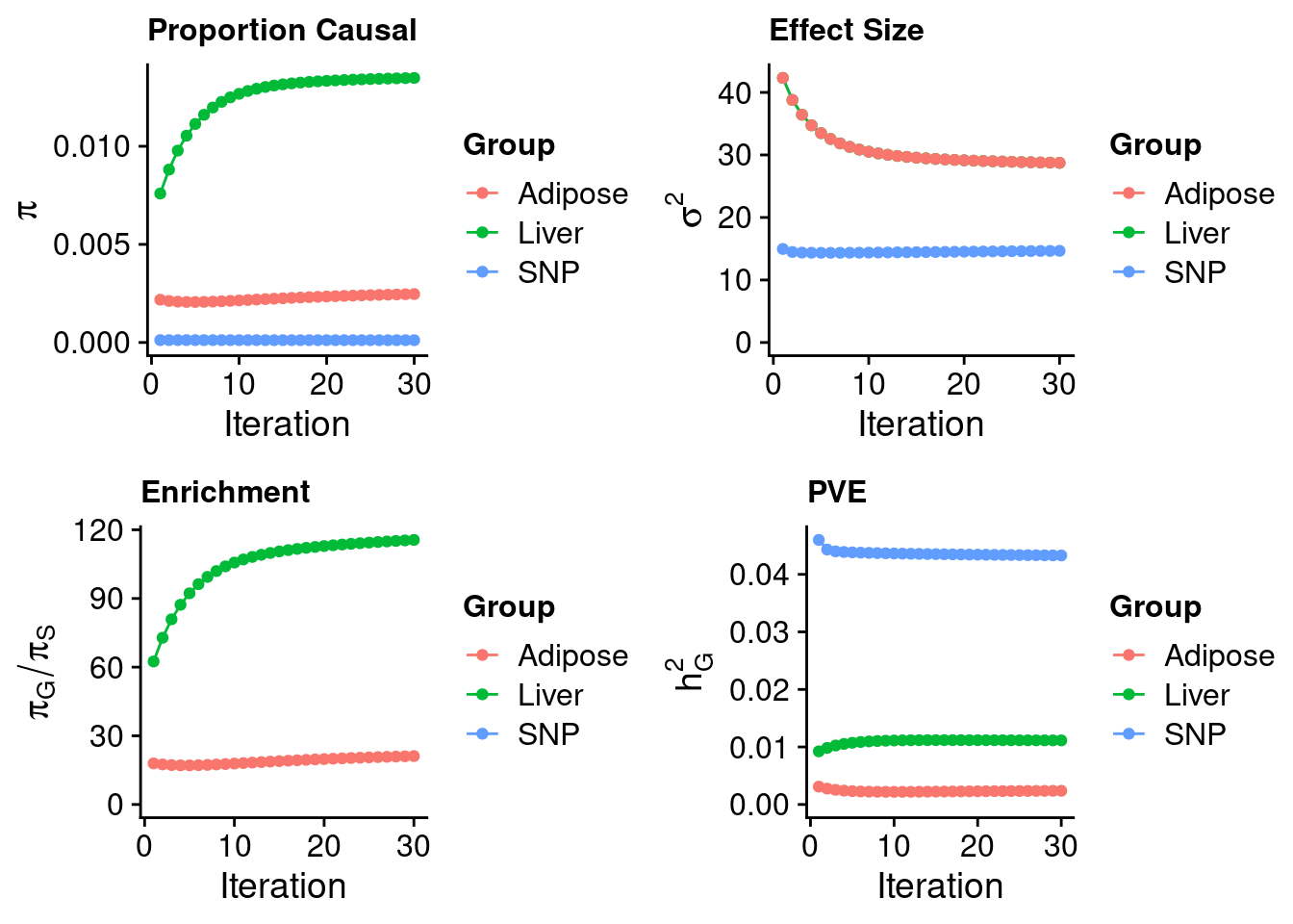
| Version | Author | Date |
|---|---|---|
| 3147f25 | wesleycrouse | 2023-09-12 |
Viewing the results
As before, we will add the gene names to the results (the PredictDB weights use Ensembl IDs as the primary identifier), as well as the z-scores for each SNP and gene. We then show all genes with PIP greater than 0.8, which is the threshold we used in the paper.
#load cTWAS results
ctwas_res <- read.table(paste0(outputdir, outname, ".susieIrss.txt"), header=T)

#load information for all genes
gene_info <- data.frame(gene=as.character(), genename=as.character(), gene_type=as.character(), weight=as.character())

for (i in 1:length(weight)){
  sqlite <- RSQLite::dbDriver("SQLite")
  db = RSQLite::dbConnect(sqlite, weight[i])
  query <- function(...) RSQLite::dbGetQuery(db, ...)
  gene_info_current <- query("select gene, genename, gene_type from extra")
  RSQLite::dbDisconnect(db)

  gene_info_current$weight <- weight[i]

  gene_info <- rbind(gene_info, gene_info_current)
}

gene_info$weight <- sapply(gene_info$weight, function(x){rev(unlist(strsplit(tools::file_path_sans_ext(x), "/")))[1]})
gene_info$id <- paste(gene_info$gene, gene_info$weight, sep="|")

#add gene names to cTWAS results
ctwas_res$genename[ctwas_res$type!="SNP"] <- gene_info$genename[match(ctwas_res$id[ctwas_res$type!="SNP"], gene_info$id)]

rm(gene_info)

#add z-scores to cTWAS results
ctwas_res$z[ctwas_res$type=="SNP"] <- z_snp$z[match(ctwas_res$id[ctwas_res$type=="SNP"], z_snp$id)]
ctwas_res$z[ctwas_res$type!="SNP"] <- z_gene$z[match(ctwas_res$id[ctwas_res$type!="SNP"], z_gene$id)]

#display the genes with PIP > 0.8
ctwas_res <- ctwas_res[order(-ctwas_res$susie_pip),]
ctwas_res[ctwas_res$type!="SNP" & ctwas_res$susie_pip > 0.8,]
chrom id pos
875456 1 ENSG00000134222.16|mashr_Liver_nolnc 109275684
1205603 16 ENSG00000261701.6|mashr_Liver_nolnc 72063820
921101 2 ENSG00000125629.14|mashr_Liver_nolnc 118088372
1300580 19 ENSG00000104870.12|mashr_Adipose_Subcutaneous_nolnc 49506216
964198 3 ENSG00000138246.15|mashr_Adipose_Subcutaneous_nolnc 132417408
917413 2 ENSG00000143921.6|mashr_Liver_nolnc 43839108
1040065 8 ENSG00000173273.15|mashr_Liver_nolnc 9315699
1153507 13 ENSG00000183087.14|mashr_Liver_nolnc 113849020
984483 6 ENSG00000204599.14|mashr_Liver_nolnc 30324306
1313921 20 ENSG00000100979.14|mashr_Liver_nolnc 45906012
930511 2 ENSG00000163083.5|mashr_Liver_nolnc 120552693
1104553 11 ENSG00000149485.18|mashr_Liver_nolnc 61829161
1286910 19 ENSG00000255974.7|mashr_Liver_nolnc 40847202
977050 5 ENSG00000151292.17|mashr_Liver_nolnc 123513182
1230060 17 ENSG00000173757.9|mashr_Liver_nolnc 42276835
897972 1 ENSG00000143771.11|mashr_Liver_nolnc 224356827
1193741 16 ENSG00000087237.10|mashr_Adipose_Subcutaneous_nolnc 56960332
1293403 19 ENSG00000105287.12|mashr_Liver_nolnc 46713856
999860 7 ENSG00000105866.13|mashr_Liver_nolnc 21553355
856283 1 ENSG00000169174.10|mashr_Adipose_Subcutaneous_nolnc 55025188
1220001 17 ENSG00000129244.8|mashr_Liver_nolnc 7646363
938094 2 ENSG00000138439.11|mashr_Adipose_Subcutaneous_nolnc 202630335
1293434 19 ENSG00000176920.11|mashr_Liver_nolnc 48700572
957720 3 ENSG00000082701.14|mashr_Liver_nolnc 120094435
1017959 7 ENSG00000136271.10|mashr_Liver_nolnc 44575121
1215803 16 ENSG00000153786.12|mashr_Adipose_Subcutaneous_nolnc 85001918
1031107 7 ENSG00000172336.4|mashr_Liver_nolnc 100705751
905490 2 ENSG00000151360.9|mashr_Liver_nolnc 3594771
964193 3 ENSG00000138246.15|mashr_Liver_nolnc 132417408
1022706 7 ENSG00000164713.9|mashr_Liver_nolnc 98253249
936104 2 ENSG00000123612.15|mashr_Liver_nolnc 157625480
868412 1 ENSG00000198890.7|mashr_Liver_nolnc 107056380
1238840 17 ENSG00000141338.13|mashr_Adipose_Subcutaneous_nolnc 68883786
847891 1 ENSG00000088280.18|mashr_Liver_nolnc 23484588
1034749 8 ENSG00000253958.1|mashr_Liver_nolnc 8535378
1055920 9 ENSG00000155158.20|mashr_Liver_nolnc 15280189
1300502 19 ENSG00000105552.14|mashr_Liver_nolnc 48811525
938084 2 ENSG00000204217.13|mashr_Liver_nolnc 202422002
1293473 19 ENSG00000142233.11|mashr_Adipose_Subcutaneous_nolnc 48702748
1308472 19 ENSG00000099326.8|mashr_Liver_nolnc 58573678
1031112 7 ENSG00000087087.18|mashr_Liver_nolnc 100875204
1127597 12 ENSG00000188906.14|mashr_Liver_nolnc 40194128
1113929 11 ENSG00000213445.9|mashr_Adipose_Subcutaneous_nolnc 65631472
1273268 19 ENSG00000105520.10|mashr_Adipose_Subcutaneous_nolnc 11354640
1074726 10 ENSG00000198964.13|mashr_Liver_nolnc 50624798
1162991 14 ENSG00000205978.5|mashr_Liver_nolnc 24400540
1042242 8 ENSG00000076554.15|mashr_Adipose_Subcutaneous_nolnc 80171625
974903 4 ENSG00000145390.11|mashr_Liver_nolnc 119212763
1187856 15 ENSG00000140564.11|mashr_Liver_nolnc 90868426
1137363 12 ENSG00000119242.8|mashr_Adipose_Subcutaneous_nolnc 123959862
1145626 13 ENSG00000244754.8|mashr_Liver_nolnc 32538827
1209951 16 ENSG00000140961.12|mashr_Liver_nolnc 83946924
1220000 17 ENSG00000141504.11|mashr_Liver_nolnc 7626953
1068293 9 ENSG00000148180.19|mashr_Liver_nolnc 121208638
1080788 10 ENSG00000166272.16|mashr_Liver_nolnc 102727686
1262590 19 ENSG00000167674.14|mashr_Liver_nolnc 4472101
1279563 19 ENSG00000130311.10|mashr_Liver_nolnc 17309356
863790 1 ENSG00000162607.12|mashr_Liver_nolnc 62436136
849865 1 ENSG00000142765.17|mashr_Liver_nolnc 27342119
994260 6 ENSG00000112339.14|mashr_Liver_nolnc 135069698
1293470 19 ENSG00000063176.15|mashr_Adipose_Subcutaneous_nolnc 48624233
1247674 18 ENSG00000119537.15|mashr_Liver_nolnc 63367187
880779 1 ENSG00000162836.11|mashr_Liver_nolnc 147646379
1050310 8 ENSG00000164938.13|mashr_Liver_nolnc 94949325
949893 3 ENSG00000168297.15|mashr_Liver_nolnc 58332534
1223261 17 ENSG00000167525.13|mashr_Adipose_Subcutaneous_nolnc 28711515
1086634 10 ENSG00000119965.12|mashr_Liver_nolnc 122945179
1187855 15 ENSG00000140577.15|mashr_Liver_nolnc 90529730
1093915 11 ENSG00000177685.16|mashr_Liver_nolnc 827713
1168762 14 ENSG00000205683.11|mashr_Liver_nolnc 72894241
1097993 11 ENSG00000179119.14|mashr_Liver_nolnc 18634724
945093 2 ENSG00000127831.10|mashr_Liver_nolnc 218419492
1313920 20 ENSG00000168612.4|mashr_Liver_nolnc 45880903
1313911 20 ENSG00000124145.6|mashr_Liver_nolnc 45338670
1252500 19 ENSG00000172009.14|mashr_Liver_nolnc 2786399
949898 3 ENSG00000198643.6|mashr_Liver_nolnc 58666565
840683 1 ENSG00000142627.12|mashr_Liver_nolnc 16156481
type region_tag1 region_tag2 cs_index susie_pip mu2
875456 Liver 1 67 1 1.0000000 1626.39733
1205603 Liver 16 38 1 0.9999997 153.94303
921101 Liver 2 69 1 0.9999974 64.04761
1300580 Adipose 19 34 2 0.9999841 1523.43860
964198 Adipose 3 82 1 0.9998215 83.00146
917413 Liver 2 27 1 0.9991814 302.62225
1040065 Liver 8 12 1 0.9986467 81.16154
1153507 Liver 13 62 1 0.9985972 77.70567
984483 Liver 6 24 1 0.9985468 75.78000
1313921 Liver 20 28 2 0.9977147 59.90758
930511 Liver 2 70 1 0.9972855 72.81400
1104553 Liver 11 34 1 0.9970792 158.79603
1286910 Liver 19 28 1 0.9960592 31.16748
977050 Liver 5 75 1 0.9955770 82.43659
1230060 Liver 17 25 1 0.9948814 31.07379
897972 Liver 1 114 1 0.9942504 40.37204
1193741 Adipose 16 31 1 0.9939986 138.71686
1293403 Liver 19 33 2 0.9938631 29.00746
999860 Liver 7 19 1 0.9938243 100.47788
856283 Adipose 1 34 3 0.9924322 114.91769
1220001 Liver 17 7 1 0.9914785 37.09339
938094 Adipose 2 120 1 0.9875333 46.99878
1293434 Liver 19 33 1 0.9870850 61.91303
957720 Liver 3 74 1 0.9851409 43.92782
1017959 Liver 7 32 2 0.9849785 57.48240
1215803 Adipose 16 49 1 0.9842259 27.93781
1031107 Liver 7 62 3 0.9840788 41.36037
905490 Liver 2 2 1 0.9835021 27.51907
964193 Liver 3 82 2 0.9801771 90.11562
1022706 Liver 7 60 1 0.9784173 29.44894
936104 Liver 2 94 1 0.9759563 24.84081
868412 Liver 1 66 1 0.9699806 31.44140
1238840 Adipose 17 39 3 0.9696022 32.07870
847891 Liver 1 16 1 0.9674202 32.26601
1034749 Liver 8 11 1 0.9582030 25.12727
1055920 Liver 9 13 1 0.9572766 22.79163
1300502 Liver 19 34 1 0.9502051 26.34479
938084 Liver 2 120 2 0.9493726 27.12936
1293473 Adipose 19 33 4 0.9490689 58.29687
1308472 Liver 19 39 2 0.9445003 30.03895
1031112 Liver 7 62 2 0.9443047 32.10793
1127597 Liver 12 25 1 0.9429438 26.52642
1113929 Adipose 11 36 1 0.9422099 26.16307
1273268 Adipose 19 10 5 0.9364037 31.84989
1074726 Liver 10 33 1 0.9325839 23.99160
1162991 Liver 14 3 1 0.9264982 48.14652
1042242 Adipose 8 57 1 0.9257452 25.71814
974903 Liver 4 77 1 0.9249822 24.03569
1187856 Liver 15 42 1 0.9145107 22.11389
1137363 Adipose 12 75 1 0.9140207 30.50941
1145626 Liver 13 11 2 0.9113481 27.33164
1209951 Liver 16 48 1 0.9056783 49.86130
1220000 Liver 17 7 0 0.9050244 24.93119
1068293 Liver 9 62 1 0.9035894 25.61959
1080788 Liver 10 66 1 0.8944034 22.12075
1262590 Liver 19 5 0 0.8925091 21.58841
1279563 Liver 19 14 0 0.8814246 22.09555
863790 Liver 1 39 1 0.8796699 251.36385
849865 Liver 1 19 1 0.8788043 21.23177
994260 Liver 6 89 1 0.8729362 28.48964
1293470 Adipose 19 33 3 0.8708694 38.75007
1247674 Liver 18 35 1 0.8698953 24.14218
880779 Liver 1 73 1 0.8695047 21.48528
1050310 Liver 8 66 1 0.8657317 21.44965
949893 Liver 3 40 2 0.8650828 27.44129
1223261 Adipose 17 17 2 0.8628298 30.72466
1086634 Liver 10 77 1 0.8560163 38.82627
1187855 Liver 15 42 0 0.8445486 22.47120
1093915 Liver 11 1 0 0.8444883 21.10145
1168762 Liver 14 34 0 0.8404494 20.93932
1097993 Liver 11 13 1 0.8370970 33.44970
945093 Liver 2 129 1 0.8282817 26.47016
1313920 Liver 20 28 0 0.8262432 30.57181
1313911 Liver 20 28 0 0.8194279 21.10817
1252500 Liver 19 3 1 0.8131890 27.50227
949898 Liver 3 40 3 0.8128006 21.47916
840683 Liver 1 11 0 0.8114200 21.75891
genename z
875456 PSRC1 -41.6873361
1205603 HPR -17.9627705
921101 INSIG2 -8.9827018
1300580 FCGRT -4.3479561
964198 DNAJC13 -3.9826268
917413 ABCG8 -20.2939818
1040065 TNKS 11.0385644
1153507 GAS6 -8.9236884
984483 TRIM39 8.8401635
1313921 PLTP -5.7324907
930511 INHBB -8.5189356
1104553 FADS1 12.9263513
1286910 CYP2A6 5.4070280
977050 CSNK1G3 9.1162909
1230060 STAT5B 5.4262521
897972 CNIH4 6.1455352
1193741 CETP 13.8144273
1293403 PRKD2 5.0722167
999860 SP4 10.6931913
856283 PCSK9 17.2108693
1220001 ATP1B2 4.7940083
938094 FAM117B 7.8526526
1293434 FUT2 -11.9271069
957720 GSK3B 6.4748241
1017959 DDX56 9.6418614
1215803 ZDHHC7 -4.8622384
1031107 POP7 -5.8452584
905490 ALLC 4.9190656
964193 DNAJC13 4.8455009
1022706 BRI3 -5.1401355
936104 ACVR1C -4.6873702
868412 PRMT6 -5.3237208
1238840 ABCA8 4.8004468
847891 ASAP3 5.2832248
1034749 CLDN23 4.7200104
1055920 TTC39B -4.3344945
1300502 BCAT2 4.7963978
938084 BMPR2 6.1242669
1293473 NTN5 11.1322519
1308472 MZF1 -4.6096568
1031112 SRRT 5.4249961
1127597 LRRK2 4.7928082
1113929 SIPA1 -5.0964929
1273268 PLPPR2 3.9656649
1074726 SGMS1 4.8739685
1162991 NYNRIN 7.0099523
1042242 TPD52 -4.6843625
974903 USP53 -4.5083710
1187856 FURIN -4.3910334
1137363 CCDC92 -5.3280459
1145626 N4BP2L2 3.8680171
1209951 OSGIN1 6.9073098
1220000 SAT2 2.6934662
1068293 GSN -4.6968606
1080788 WBP1L -4.2557557
1262590 CTB-50L17.10 4.2586633
1279563 DDA1 4.7740307
863790 USP1 16.2582110
849865 SYTL1 -3.9628543
994260 HBS1L 5.0222452
1293470 SPHK2 -8.7214595
1247674 KDSR -4.5262867
880779 ACP6 4.0601206
1050310 TP53INP1 4.0384478
949893 PXK -3.7920082
1223261 PROCA1 5.5432820
1086634 C10orf88 -6.7878497
1187855 CRTC3 -4.3895585
1093915 CRACR2B -3.9895855
1168762 DPF3 -3.8928948
1097993 SPTY2D1 -5.5571227
945093 VIL1 4.7255312
1313920 ZSWIM1 -0.6413199
1313911 SDC4 -3.9207271
1252500 THOP1 4.9057397
949898 FAM3D -3.8894573
840683 EPHA2 -4.0941586In the context of genes in multiple tissues, it is also useful to evaluate the PIP for each gene combined over tissues:
#aggregate by gene name
df_gene <- aggregate(ctwas_res$susie_pip[ctwas_res$type!="SNP"], by=list(ctwas_res$genename[ctwas_res$type!="SNP"]), FUN=sum)
colnames(df_gene) <- c("genename", "combined_pip")

#drop duplicated gene names
df_gene <- df_gene[!(df_gene$genename %in% names(which(table(ctwas_res$genename)>length(weight)))),]

#collect tissue-level results
all_tissue_names <- unique(ctwas_res$type[ctwas_res$type!="SNP"])

df_gene_pips <- matrix(NA, nrow=nrow(df_gene), ncol=length(all_tissue_names))
colnames(df_gene_pips) <- all_tissue_names

ctwas_gene_res <- ctwas_res[ctwas_res$type!="SNP",]

for (i in 1:nrow(df_gene)){
  gene <- df_gene$genename[i]
  ctwas_gene_res_subset <- ctwas_gene_res[which(ctwas_gene_res$genename==gene),]
  df_gene_pips[i,ctwas_gene_res_subset$type] <- ctwas_gene_res_subset$susie_pip
}

df_gene <- cbind(df_gene, df_gene_pips)

rm(df_gene_pips, ctwas_gene_res, ctwas_gene_res_subset)

#sort by combined PIP
df_gene <- df_gene[order(-df_gene$combined_pip),]
df_gene <- df_gene[,apply(df_gene, 2, function(x){!all(is.na(x))})] #drop genes that weren't imputed in any tissue

#genes with PIP>0.8 or 20 highest PIPs
head(df_gene, max(sum(df_gene$combined_pip>0.8), 20))
genename combined_pip Liver Adipose
3176 DNAJC13 1.9799986 9.801771e-01 9.998215e-01
191 ACVR1C 1.1261346 9.759563e-01 1.501783e-01
2149 CETP 1.1169933 1.229948e-01 9.939986e-01
12731 ZDHHC7 1.0620377 7.781184e-02 9.842259e-01
8820 PSRC1 1.0075935 1.000000e+00 7.593502e-03
4358 GAS6 1.0060571 9.985972e-01 7.459953e-03
8064 PELO 1.0035760 5.024904e-01 5.010856e-01
2692 CSNK1G3 1.0031056 9.955770e-01 7.528617e-03
5375 INHBB 1.0012097 9.972855e-01 3.924139e-03
5391 INSIG2 1.0011505 9.999974e-01 1.153056e-03
5107 HPR 1.0010150 9.999997e-01 1.015291e-03
11856 TRIM39 1.0008417 9.985468e-01 2.294848e-03
4057 FCGRT 1.0000238 3.973914e-05 9.999841e-01
60 ABCG8 0.9991814 9.991814e-01 NA
8374 PLTP 0.9989467 9.977147e-01 1.231980e-03
11690 TNKS 0.9986467 9.986467e-01 NA
2829 CYP2A6 0.9980887 9.960592e-01 2.029523e-03
2411 CNIH4 0.9975962 9.942504e-01 3.345786e-03
10846 STAT5B 0.9972770 9.948814e-01 2.395582e-03
3765 FADS1 0.9970792 9.970792e-01 NA
10614 SP4 0.9966978 9.938243e-01 2.873506e-03
918 ATP1B2 0.9966460 9.914785e-01 5.167490e-03
8679 PRKD2 0.9942458 9.938631e-01 3.827365e-04
7977 PCSK9 0.9924322 NA 9.924322e-01
10730 SPTY2D1 0.9918087 8.370970e-01 1.547116e-01
1267 C10orf88 0.9890884 8.560163e-01 1.330721e-01
2990 DDX56 0.9887973 9.849785e-01 3.818732e-03
458 ALLC 0.9876085 9.835021e-01 4.106457e-03
3793 FAM117B 0.9875333 NA 9.875333e-01
4275 FUT2 0.9870850 9.870850e-01 NA
4754 GSK3B 0.9851409 9.851409e-01 NA
5662 KDSR 0.9850219 8.698953e-01 1.151266e-01
8486 POP7 0.9840788 9.840788e-01 NA
10765 SRRT 0.9823611 9.443047e-01 3.805641e-02
1205 BRI3 0.9815273 9.784173e-01 3.110027e-03
2774 CWF19L1 0.9805764 7.658773e-01 2.146991e-01
1814 CCDC92 0.9761439 6.212321e-02 9.140207e-01
8264 PKN3 0.9750684 6.572158e-01 3.178526e-01
7960 PCMTD2 0.9705038 2.739162e-01 6.965876e-01
8691 PRMT6 0.9699806 9.699806e-01 NA
824 ASAP3 0.9697683 9.674202e-01 2.348021e-03
31 ABCA8 0.9696022 NA 9.696022e-01
8368 PLPPR2 0.9679011 3.149742e-02 9.364037e-01
10086 SIPA1 0.9674107 2.520088e-02 9.422099e-01
2315 CLDN23 0.9600289 9.582030e-01 1.825925e-03
12011 TTC39B 0.9599800 9.572766e-01 2.703350e-03
1169 BMPR2 0.9535796 9.493726e-01 4.207004e-03
7086 MZF1 0.9509912 9.445003e-01 6.490953e-03
1084 BCAT2 0.9502081 9.502051e-01 3.032018e-06
7562 NTN5 0.9490689 NA 9.490689e-01
11522 TMEM199 0.9481945 7.114751e-01 2.367194e-01
6210 LRRK2 0.9458186 9.429438e-01 2.874851e-03
9552 RPS11 0.9446817 7.985254e-01 1.461563e-01
10673 SPHK2 0.9443445 7.347516e-02 8.708694e-01
7458 NPC1L1 0.9392186 7.929435e-01 1.462750e-01
5840 KPNA1 0.9367328 2.536761e-01 6.830568e-01
11756 TPD52 0.9358023 1.005711e-02 9.257452e-01
9998 SGMS1 0.9325839 9.325839e-01 NA
7645 NYNRIN 0.9295386 9.264982e-01 3.040334e-03
12315 USP53 0.9292979 9.249822e-01 4.315735e-03
5779 KLHDC7A 0.9252255 7.807753e-01 1.444502e-01
4270 FURIN 0.9166055 9.145107e-01 2.094804e-03
7093 N4BP2L2 0.9128246 9.113481e-01 1.476541e-03
1850 CCND2 0.9098426 6.982195e-01 2.116231e-01
7741 OSGIN1 0.9077131 9.056783e-01 2.034796e-03
9727 SAT2 0.9070538 9.050244e-01 2.029470e-03
10591 SORCS2 0.9050890 4.337048e-01 4.713842e-01
4756 GSN 0.9035894 9.035894e-01 NA
8697 PROCA1 0.9001486 3.731878e-02 8.628298e-01
12463 WBP1L 0.8993326 8.944034e-01 4.929153e-03
2714 CTB-50L17.10 0.8960038 8.925091e-01 3.494657e-03
147 ACP6 0.8866123 8.695047e-01 1.710757e-02
12283 USP1 0.8838901 8.796699e-01 4.220161e-03
11022 SYTL1 0.8822972 8.788043e-01 3.492915e-03
2950 DDA1 0.8814246 8.814246e-01 NA
4878 HBS1L 0.8749648 8.729362e-01 2.028607e-03
1278 C11orf58 0.8746984 7.383461e-01 1.363523e-01
5088 HOXB6 0.8730426 7.957469e-01 7.729575e-02
11746 TP53INP1 0.8686028 8.657317e-01 2.871084e-03
8924 PXK 0.8662626 8.650828e-01 1.179817e-03
2883 DAGLB 0.8636445 7.289249e-01 1.347196e-01
2620 CRACR2B 0.8568250 8.444883e-01 1.233675e-02
2666 CRTC3 0.8467871 8.445486e-01 2.238508e-03
3241 DPF3 0.8404494 8.404494e-01 NA
12373 VIL1 0.8282817 8.282817e-01 NA
13261 ZSWIM1 0.8278246 8.262432e-01 1.581360e-03
11310 THOP1 0.8228751 8.131890e-01 9.686012e-03
9807 SDC4 0.8203788 8.194279e-01 9.508738e-04
3912 FAM3D 0.8128006 8.128006e-01 NA
3588 EPHA2 0.8114200 8.114200e-01 NANOTE: To visualize individual loci, the
ctwas_locus_plot function will need to be updated to
accommodate multiple groups.
Converting between FUSION and PredictDB format
Because multiple sets of prediction models can only be specified in PredictDB format, it may be necessary to convert FUSION format weights to PredictDB format. See Jing’s code for converting between FUSION and PredictDB weights.
PredictDB weights assume that variant genotypes are not standardized
before imputation, but our implementation assumes standardized variant
genotypes. For this reason, PredictDB weights are be scaled by genotype
variance before imputing gene expression by default. If converting from
FUSION to PredictDB format, the weights are already on the standardized
scale, and scaling should be turned off using the option
scale_by_ld_variance=F in the impute_expr_z
function.
Harmonizing prediction models and LD reference
When using multiple sets of prediction models, or using the same
combination of prediction models and LD reference multiple times, it may
be beneficial to harmonize the prediction models and LD reference before
the analysis, rather than harmonizing within the
impute_expr_z function. Harmonization only needs to be done
once per combination of prediction models and LD reference. Harmonizing
beforehand reduces redundant computation, allows larger analyses to be
subdivided into smaller chunks, and allows harmonization to be
paralleled over .db files in separate jobs. Note that we
have not included an option to parallelize harmonization within
.db files in this function, as we have within the
impute_expr_z function. This is because the runtime is
manageable: pre-harmonizing the two .db files in this
analysis took around 2-3 hours each. The output is a harmonized
.db file in the output directory; we do not return the
harmonized covariances between variants in the prediction models
(.txt.gz).
preharmonize_wgt_ld(weight="weights_nolnc/mashr_Liver_nolnc.db",
                    ld_R_dir = ld_R_dir,
                    outputdir = "weights_nolnc/",
                    outname = "mashr_Liver_nolnc_harmonized",
                    strand_ambig_action_wgt = "recover")

preharmonize_wgt_ld(weight="weights_nolnc/mashr_Adipose_Subcutaneous_nolnc.db",
                    ld_R_dir = ld_R_dir,
                    outputdir = "weights_nolnc/",
                    outname = "mashr_Adipose_Subcutaneous_nolnc_harmonized",
                    strand_ambig_action_wgt = "recover")
After harmonization, we specify the harmonized weights as a vector
and run the imputation step with the weight harmonization option turned
off. The output of these commands is identical to harmonizing within the
impute_expr_z function, although the genes are now named
after the “_harmonized” .db files. These two steps can
replace the imputation step in the “Imputing gene z-scores” section.
#back up z_gene without pre-harmonization from previous sections for comparison
z_gene_orig <- z_gene

####################

weight <- c("weights_nolnc/mashr_Liver_nolnc_harmonized.db", "weights_nolnc/mashr_Adipose_Subcutaneous_nolnc_harmonized.db")

outname <- "example_multigroup_preharm"

ncore <- 6

#impute gene z-scores for both sets of prediction weights by chromosome
for (i in 1:22){
  if (!file.exists(paste0(outputdir, outname, "_chr", i, ".expr.gz"))){
    res <- impute_expr_z(z_snp = z_snp,
                         weight = weight,
                         ld_R_dir = ld_R_dir,
                         outputdir = outputdir,
                         outname = outname,
                         harmonize_z = F,
                         harmonize_wgt = F,
                         ncore=ncore,
                         chrom=i)
  }
}

#combine the imputed gene z-scores
ld_exprfs <- paste0(outputdir, outname, "_chr", 1:22, ".expr.gz")

z_gene <- list()

for (i in 1:22){
  load(paste0(outputdir, outname, "_chr", i, ".exprqc.Rd"))
  z_gene[[i]] <- z_gene_chr
}

z_gene <- do.call(rbind, z_gene)
rownames(z_gene) <- NULL

rm(qclist, wgtlist, z_gene_chr)

####################

#compare z_gene and z_gene_orig
head(z_gene)
id z
1 ENSG00000203995.9|mashr_Liver_nolnc_harmonized 1.3215822
2 ENSG00000178965.13|mashr_Liver_nolnc_harmonized 0.2323771
3 ENSG00000073754.5|mashr_Liver_nolnc_harmonized 0.1452688
4 ENSG00000158764.6|mashr_Liver_nolnc_harmonized 0.5230683
5 ENSG00000143195.12|mashr_Liver_nolnc_harmonized -0.7138027
6 ENSG00000143194.12|mashr_Liver_nolnc_harmonized 0.8676492head(z_gene_orig) id z type
1 ENSG00000203995.9|mashr_Liver_nolnc 1.3215822 Liver
2 ENSG00000178965.13|mashr_Liver_nolnc 0.2323771 Liver
3 ENSG00000073754.5|mashr_Liver_nolnc 0.1452688 Liver
4 ENSG00000158764.6|mashr_Liver_nolnc 0.5230683 Liver
5 ENSG00000143195.12|mashr_Liver_nolnc -0.7138027 Liver
6 ENSG00000143194.12|mashr_Liver_nolnc 0.8676492 Liver#match gene names; preharmonized version has an additional "_harmonized" from the .db file name
z_gene_orig <- z_gene_orig[sapply(z_gene_orig$id, grep, x=z_gene$id, fixed=T),]
any(z_gene_orig$z!=z_gene$z)[1] FALSE
sessionInfo()R version 4.1.0 (2021-05-18)
Platform: x86_64-pc-linux-gnu (64-bit)
Running under: CentOS Linux 7 (Core)
Matrix products: default
BLAS: /software/R-4.1.0-no-openblas-el7-x86_64/lib64/R/lib/libRblas.so
LAPACK: /software/R-4.1.0-no-openblas-el7-x86_64/lib64/R/lib/libRlapack.so
locale:
[1] LC_CTYPE=en_US.UTF-8 LC_NUMERIC=C LC_TIME=C
[4] LC_COLLATE=C LC_MONETARY=C LC_MESSAGES=C
[7] LC_PAPER=C LC_NAME=C LC_ADDRESS=C
[10] LC_TELEPHONE=C LC_MEASUREMENT=C LC_IDENTIFICATION=C
attached base packages:
[1] stats graphics grDevices utils datasets methods base
other attached packages:
[1] cowplot_1.1.1 ggplot2_3.4.0 ctwas_0.1.40 workflowr_1.7.0
loaded via a namespace (and not attached):
[1] Rcpp_1.0.11 lattice_0.20-45 getPass_0.2-2 ps_1.7.2
[5] assertthat_0.2.1 rprojroot_2.0.3 digest_0.6.31 foreach_1.5.2
[9] utf8_1.2.3 R6_2.5.1 RSQLite_2.3.1 evaluate_0.18
[13] httr_1.4.4 highr_0.9 pillar_1.9.0 rlang_1.1.1
[17] rstudioapi_0.14 data.table_1.14.8 whisker_0.4.1 callr_3.7.3
[21] jquerylib_0.1.4 blob_1.2.4 Matrix_1.5-3 rmarkdown_2.18
[25] labeling_0.4.2 stringr_1.5.0 bit_4.0.5 munsell_0.5.0
[29] compiler_4.1.0 httpuv_1.6.6 xfun_0.35 pkgconfig_2.0.3
[33] htmltools_0.5.4 tidyselect_1.2.0 tibble_3.2.1 logging_0.10-108
[37] codetools_0.2-18 fansi_1.0.4 dplyr_1.0.10 withr_2.5.0
[41] later_1.3.0 grid_4.1.0 jsonlite_1.8.4 gtable_0.3.1
[45] lifecycle_1.0.3 DBI_1.1.3 git2r_0.30.1 magrittr_2.0.3
[49] scales_1.2.1 cli_3.6.1 stringi_1.7.8 cachem_1.0.8
[53] farver_2.1.1 fs_1.5.2 promises_1.2.0.1 pgenlibr_0.3.6
[57] bslib_0.4.1 generics_0.1.3 vctrs_0.6.3 iterators_1.0.14
[61] tools_4.1.0 bit64_4.0.5 glue_1.6.2 processx_3.8.0
[65] fastmap_1.1.1 yaml_2.3.6 colorspace_2.0-3 memoise_2.0.1
[69] knitr_1.41 sass_0.4.4