Using cTWAS
wesleycrouse
2023-08-31
Last updated: 2023-09-12
Checks: 6 1
Knit directory: ctwas_applied/
This reproducible R Markdown analysis was created with workflowr (version 1.7.0). The Checks tab describes the reproducibility checks that were applied when the results were created. The Past versions tab lists the development history.
The R Markdown file has unstaged changes. To know which version of
the R Markdown file created these results, you’ll want to first commit
it to the Git repo. If you’re still working on the analysis, you can
ignore this warning. When you’re finished, you can run
wflow_publish to commit the R Markdown file and build the
HTML.
Great job! The global environment was empty. Objects defined in the global environment can affect the analysis in your R Markdown file in unknown ways. For reproduciblity it’s best to always run the code in an empty environment.
The command set.seed(20210726) was run prior to running
the code in the R Markdown file. Setting a seed ensures that any results
that rely on randomness, e.g. subsampling or permutations, are
reproducible.
Great job! Recording the operating system, R version, and package versions is critical for reproducibility.
Nice! There were no cached chunks for this analysis, so you can be confident that you successfully produced the results during this run.
Great job! Using relative paths to the files within your workflowr project makes it easier to run your code on other machines.
Great! You are using Git for version control. Tracking code development and connecting the code version to the results is critical for reproducibility.
The results in this page were generated with repository version f2b5c01. See the Past versions tab to see a history of the changes made to the R Markdown and HTML files.
Note that you need to be careful to ensure that all relevant files for
the analysis have been committed to Git prior to generating the results
(you can use wflow_publish or
wflow_git_commit). workflowr only checks the R Markdown
file, but you know if there are other scripts or data files that it
depends on. Below is the status of the Git repository when the results
were generated:
Untracked files:
    Untracked:  gwas.RData
    Untracked:  ld_R_info.RData
    Untracked:  z_snp_pos_ebi-a-GCST004131.RData
    Untracked:  z_snp_pos_ebi-a-GCST004132.RData
    Untracked:  z_snp_pos_ebi-a-GCST004133.RData
    Untracked:  z_snp_pos_scz-2018.RData
    Untracked:  z_snp_pos_ukb-a-360.RData
    Untracked:  z_snp_pos_ukb-d-30780_irnt.RData

Unstaged changes:
    Modified:   analysis/index.Rmd
    Modified:   analysis/transition.Rmd
    Modified:   analysis/transition_multigroup.Rmd
    Modified:   code/automate_Rmd.R
Note that any generated files, e.g. HTML, png, CSS, etc., are not included in this status report because it is ok for generated content to have uncommitted changes.
These are the previous versions of the repository in which changes were
made to the R Markdown (analysis/transition.Rmd) and HTML
(docs/transition.html) files. If you’ve configured a remote
Git repository (see ?wflow_git_remote), click on the
hyperlinks in the table below to view the files as they were in that
past version.
| File | Version | Author | Date | Message |
|---|---|---|---|---|
| Rmd | f2b5c01 | wesleycrouse | 2023-09-05 | adding region merging section to the transition document |
| html | f2b5c01 | wesleycrouse | 2023-09-05 | adding region merging section to the transition document |
| Rmd | a764e3d | wesleycrouse | 2023-08-31 | ctwas user guide |
| html | a764e3d | wesleycrouse | 2023-08-31 | ctwas user guide |
| Rmd | e3b2903 | wesleycrouse | 2023-08-31 | adding transition documents |
Overview
This document is a user guide for the cTWAS R package. It details how to use to use the summary statistics version of cTWAS, which is an integrative method for identifying causal genes at GWAS loci using eQTL data. Briefly, cTWAS conditions on genetic confounders, jointly modeling sparse effects of all nearby genes and variants in an extended fine-mapping framework. Additional details are available in the paper.
Running cTWAS involves four main steps: preparing input data, imputing gene z-scores, estimating parameters, and fine-mapping the genes and variants. The output of cTWAS is a posterior inclusion probability (PIP) for each variant and each gene with an expression model. This document will cover each of these topics in detail. We also describe some of the options available at each step and the analysis considerations behind these options.
We will start by examining the input data and running the cTWAS fine-mapping step at a single locus using parameters previously estimated in the cTWAS paper. Running cTWAS with fixed parameters at a single locus is relatively fast, and is the simplest way to use cTWAS, but it requires specifying parameters, rather than learning them from the data.
We will then provide a workflow for the same analysis, but using the full data and estimating parameters. This can be computationally intensive. We performed these analyses for the paper with 10 cores and 56GB of RAM, although the exact resource requirements will vary with the numbers of genes and variants provided.
Getting started
Start by installing cTWAS in R via GitHub. For the first section of this document, we will use the main branch of cTWAS.
remotes::install_github("xinhe-lab/ctwas", ref = "main")Then load the package and set the working directory where you want to perform perform the analysis.
library(ctwas)

#set the working directory interactively
setwd("/project2/mstephens/wcrouse/ctwas_tutorial")

#set the working directory when compiling this document with Knitr
knitr::opts_knit$set(root.dir = "/project2/mstephens/wcrouse/ctwas_tutorial")
Preparing input data
The inputs for the summary statistics version of cTWAS include GWAS summary statistics for variants, prediction models for genes, and an LD reference.
These inputs should be harmonized prior to analysis (i.e. the reference and alternative alleles for each variant should match across all three data sources). We provide some options for harmonization during the gene imputation step if the data are not already harmonized. See the section on harmonization for more details.
GWAS z-scores
For this analysis, we will use summary statistics from a GWAS of LDL cholesterol in the UK Biobank. We will download the VCF from the IEU Open GWAS Project. Set the working directory, download the summary statistics, and unzip the file.
dir.create("gwas_summary_stats")

system("wget https://gwas.mrcieu.ac.uk/files/ukb-d-30780_irnt/ukb-d-30780_irnt.vcf.gz -P gwas_summary_stats")
R.utils::gunzip("gwas_summary_stats/ukb-d-30780_irnt.vcf.gz")
Next, we will use the VariantAnnotation package to read the summary statistics. Then, we will compute the z-scores and format the input data. We will also collect the sample size, which will be useful later. We will save this output for convenience.
#read the data
z_snp <- VariantAnnotation::readVcf("gwas_summary_stats/ukb-d-30780_irnt.vcf")
z_snp <- as.data.frame(gwasvcf::vcf_to_tibble(z_snp))

#compute the z-scores
z_snp$Z <- z_snp$ES/z_snp$SE

#collect sample size (most frequent sample size for all variants)
gwas_n <- as.numeric(names(sort(table(z_snp$SS),decreasing=TRUE)[1]))

#subset the columns and format the column names
z_snp <- z_snp[,c("rsid", "ALT", "REF", "Z")]
colnames(z_snp) <- c("id", "A1", "A2", "z")

#drop multiallelic variants (id not unique)
z_snp <- z_snp[!(z_snp$id %in% z_snp$id[duplicated(z_snp$id)]),]

#save the formatted z-scores and GWAS sample size
saveRDS(z_snp, file="gwas_summary_stats/ukb-d-30780_irnt.RDS")
saveRDS(gwas_n, file="gwas_summary_stats/gwas_n.RDS")
After the previous step has run, we can load the data and look at the format. Z_snp is a data frame, and each row is a variant. A1 is the alternate allele, and A2 is the reference allele. The sample size for this GWAS is N=343,621.
z_snp <- readRDS("gwas_summary_stats/ukb-d-30780_irnt.RDS")
gwas_n <- readRDS("gwas_summary_stats/gwas_n.RDS")

head(z_snp)
id A1 A2 z
1 rs530212009 C CA -1.10726803
2 rs12238997 G A -1.05210759
3 rs371890604 C G -1.27724687
4 rs144155419 A G -0.84645309
5 rs189787166 T A -0.05504189
6 rs148120343 C T -1.23068731gwas_n[1] 343621Prediction models
Prediction models can be specified in either FUSION or PredictDB format. Given a choice, PredictDB is the recommended format as some optional features are not implemented for FUSION. In this user guide, we will use PredictDB weights.
Note: cTWAS performs best when prediction models are sparse (i.e. they do not include many variants per gene). As the density of variants increases, it become more intensive to compute gene-by-gene correlations using summary statistics. Dense variants can also lead to excessive region merging. See the section on region merging for more details. Given an option, it is preferable to choose sparse prediction models for these reasons. If using dense prediction models, we recommend removing variants with weight below a threshold from the prediction models.
NOTE: It might be useful to give users the option to threshold weights during imputation.
FUSION format
Please check Fusion/TWAS for the format of FUSION weights. Below is an example.
weight_fusion <- system.file("extdata/example_fusion_weights", "Tissue", package = "ctwas")To specify weights in FUSION format, provide the directory that
contains all the .rdata files as above. We assume a file
with same name as the directory with the suffix .pos is
present in the same level as the directory. The program will search for
this file automatically. For example, we have both the directory
Tissue/ and Tissue.pos present under the
extdata/example_fusion_weights folder.
#directory and .pos file
list.files(dirname(weight_fusion))
[1] "Tissue" "Tissue.pos"#.rda files
list.files(weight_fusion) [1] "Tissue.gene1.wgt.RDat" "Tissue.gene10.wgt.RDat" "Tissue.gene11.wgt.RDat"
[4] "Tissue.gene12.wgt.RDat" "Tissue.gene13.wgt.RDat" "Tissue.gene14.wgt.RDat"
[7] "Tissue.gene15.wgt.RDat" "Tissue.gene16.wgt.RDat" "Tissue.gene17.wgt.RDat"
[10] "Tissue.gene18.wgt.RDat" "Tissue.gene19.wgt.RDat" "Tissue.gene2.wgt.RDat"
[13] "Tissue.gene20.wgt.RDat" "Tissue.gene3.wgt.RDat" "Tissue.gene4.wgt.RDat"
[16] "Tissue.gene5.wgt.RDat" "Tissue.gene6.wgt.RDat" "Tissue.gene7.wgt.RDat"
[19] "Tissue.gene8.wgt.RDat" "Tissue.gene9.wgt.RDat" rm(weight_fusion)PredictDB format
Please check PredictDB for the
format of PredictDB weights. To specify weights in PredictDB format,
provide the path to the .db file.
For this analysis, we will use liver gene expression models trained
on GTEx v8 in the PredictDB format. We will download both the prediction
models (.db) and the covariances between variants in the
prediction models (.txt.gz). The covariances can optionally
be used during harmonization to recover strand ambiguous variants.
#download the files
system("wget https://zenodo.org/record/3518299/files/mashr_eqtl.tar")

#extract to ./weights folder
system("mkdir weights")
system("tar -xvf mashr_eqtl.tar -C weights")
system("rm mashr_eqtl.tar")
In the paper, we used PredictDB models for liver gene expression. We also performed an additional preprocessing step to remove lncRNAs from the prediction models. This can be done using the following code:
library(RSQLite)

#specify the weight to remove lncRNA from
weight <- "weights/eqtl/mashr/mashr_Liver.db"

#read the PredictDB weights
sqlite <- dbDriver("SQLite")
db = dbConnect(sqlite, weight)
query <- function(...) dbGetQuery(db, ...)
weights_table <- query("select * from weights")
extra_table <- query("select * from extra")
dbDisconnect(db)

#subset to protein coding genes only
extra_table <-  extra_table[extra_table$gene_type=="protein_coding",,drop=F]
weights_table <- weights_table[weights_table$gene %in% extra_table$gene,]

#read and subset the covariances
weight_info = read.table(gzfile(paste0(tools::file_path_sans_ext(weight), ".txt.gz")), header = T)
weight_info <- weight_info[weight_info$GENE %in% extra_table$gene,]

#write the .db file and the covariances
dir.create("weights_nolnc", showWarnings=F)

if (!file.exists("weights_nolnc/mashr_Liver_nolnc.db")){
  db <- dbConnect(sqlite, "weights_nolnc/mashr_Liver_nolnc.db")
  dbWriteTable(db, "extra", extra_table)
  dbWriteTable(db, "weights", weights_table)
  dbDisconnect(db)

  weight_info_gz <- gzfile("weights_nolnc/mashr_Liver_nolnc.txt.gz", "w")
  write.table(weight_info, weight_info_gz, sep=" ", quote=F, row.names=F, col.names=T)
  close(weight_info_gz)
}

#specify the weight for the analysis
weight <- "weights_nolnc/mashr_Liver_nolnc.db"
To speed computation in our single locus example, we will also subset the prediction models to only the genes at the HPR locus that we analyzed in the paper. Subsetting the prediction models is not strictly necessary (simply specifying a single region for the fine-mapping step will yield the same output), but subsetting the weights lets us avoid imputing all the genes during the imputation step.
NOTE: Consider adding an option to impute only specific genes in the imputation function, or to impute only genes in specific regions. This will make the code more accessible for user who want to run cTWAS as a single locus with fixed parameters.
#specify the genes to subset to:
gene_subset <-  c("CMTR2", "ZNF23", "CHST4", "ZNF19", "TAT", "MARVELD3", "PHLPP2", "ATXN1L", "ZNF821", "PKD1L3", "HPR" )

#subset to selected genes only
extra_table <-  extra_table[extra_table$genename %in% gene_subset,,drop=F]
weights_table <- weights_table[weights_table$gene %in% extra_table$gene,]

#subset the covariances
weight_info <- weight_info[weight_info$GENE %in% extra_table$gene,]

#write the .db file and the covariances
if (!file.exists("weights_nolnc/mashr_Liver_nolnc_subset.db")){
  db <- dbConnect(sqlite, "weights_nolnc/mashr_Liver_nolnc_subset.db")
  dbWriteTable(db, "extra", extra_table)
  dbWriteTable(db, "weights", weights_table)
  dbDisconnect(db)

  weight_info_gz <- gzfile("weights_nolnc/mashr_Liver_nolnc_subset.txt.gz", "w")
  write.table(weight_info, weight_info_gz, sep=" ", quote=F, row.names=F, col.names=T)
  close(weight_info_gz)
}

#specify the weight for the analysis
weight_subset <- "weights_nolnc/mashr_Liver_nolnc_subset.db"
We also included this final subset of liver prediction models in the cTWAS package.
weight_subset <- system.file("extdata/weights_nolnc", "mashr_Liver_nolnc_subset.db", package = "ctwas")LD reference and regions
LD reference information can be provided to cTWAS as either individual-level genotype data (in PLINK format), or as genetic correlation matrices (termed “R matrices”) for regions that are approximately LD-independent. These regions must also be specified, regardless of how the LD reference information is provided.
cTWAS performs its analysis region-by-region. If individual-level genotype data is used for the LD reference, variants are assigned to regions, and then correlations matrices are computed within each region at each iteration of the algorithm. This can be computationally expensive if there are many individuals or if variants in the LD reference are dense. For this reason, the preferred way to run cTWAS is to provide pre-computed LD matrices for each region.
It is critical that the genome build (e.g. hg38) of the LD reference match the genome build used to train the prediction models. If the genome builds are mismatched, it is possible that variants included in a prediction model for a gene are not near the gene in the LD reference. This can lead to issues with excessive region merging. See the section on region merging for more details. The genome build of the GWAS summary statistics does not matter because variant positions are determined by the LD reference.
The choice of LD reference population is important for fine-mapping. Best practice for fine-mapping is to use an in-sample LD reference (LD computed using the subjects in the GWAS sample). If an in-sample LD reference is not an option, the LD reference should be as representative of the population in the GWAS sample as possible. Given that cTWAS is an extended fine-mapping algorithm, and that gene z-scores are computed using the observed GWAS z-scores, which reflect patterns of LD in the GWAS population, our recommendation is to match the LD reference to the GWAS population, not the population used to build the prediction models.
Regions
cTWAS includes pre-defined regions based on European (EUR), Asian
(ASN), or African (AFR) populations, using either genome build b38 or
b37. These regions were previously generated using LDetect. These
regions are specified in ctwas_rss function using the
ld_regions and ld_regions_version arguments,
respectively. The regions are left closed and right open, i.e. [start,
stop). We will open the b38 European region file to view the format,
centered on the region that we will analyze later:
regions <- system.file("extdata/ldetect", "EUR.b38.bed", package = "ctwas")

regions_df <- read.table(regions, header = T)

locus_chr <- "chr16"
locus_start <- 71020125

regions_df[which(regions_df$chr==locus_chr & regions_df$start==locus_start)+c(-2:2),]
chr start stop
1463 chr16 65904663 68807460
1464 chr16 68807460 71020125
1465 chr16 71020125 72901251
1466 chr16 72901251 74937605
1467 chr16 74937605 75944056rm(regions)Note that the default behavior of cTWAS is to merge regions that have
a gene spanning the region boundary (merge=T). For this
reason, the regions specified here may not correspond exactly to the
final regions analyzed by cTWAS. See the section on region merging for
more details.
It is also possible to specify custom regions using
ld_regions_custom in .bed format. We will make
a custom region file that includes only the region containing the HPR
locus that we analyzed in the paper.
regions_df <- regions_df[regions_df$chr==locus_chr & regions_df$start==locus_start,]

dir.create("regions", showWarnings=F)
regions_file <- "regions/regions_subset.bed"
write.table(regions_df, file=regions_file, row.names=F, col.names=T, sep="\t", quote = F)

rm(regions_df)
Genotypes
To use individual genotypes for the LD reference, provide a character
vector of .pgen or .bed files. There should be
one file per chromosome, ordered from 1 to 22. If .pgen
files are specified, then .pvar and .psam
files must also be in the same directory. If .bed files are
specified, then .bim and .fam files must also
be in the same directory. We include an example here:
ld_pgenfs <- system.file("extdata/example_genotype_files", paste0("example_chr", 1:22, ".pgen"), package = "ctwas")
head(ld_pgenfs)
[1] "/home/wcrouse/R/x86_64-pc-linux-gnu-library/4.1/ctwas/extdata/example_genotype_files/example_chr1.pgen"
[2] "/home/wcrouse/R/x86_64-pc-linux-gnu-library/4.1/ctwas/extdata/example_genotype_files/example_chr2.pgen"
[3] "/home/wcrouse/R/x86_64-pc-linux-gnu-library/4.1/ctwas/extdata/example_genotype_files/example_chr3.pgen"
[4] "/home/wcrouse/R/x86_64-pc-linux-gnu-library/4.1/ctwas/extdata/example_genotype_files/example_chr4.pgen"
[5] "/home/wcrouse/R/x86_64-pc-linux-gnu-library/4.1/ctwas/extdata/example_genotype_files/example_chr5.pgen"
[6] "/home/wcrouse/R/x86_64-pc-linux-gnu-library/4.1/ctwas/extdata/example_genotype_files/example_chr6.pgen"rm(ld_pgenfs)LD matrices
To use LD matrices for the LD reference, provide a directory
containing all of the .RDS matrix files and matching
.Rvar variant information files. We have included an LD
matrix for the HPR locus that we analyzed in the paper as part of the
package. The complete LD matrix for this region was too large to include
in the package, so we include only half of the variants at this locus,
including the ones needed for the prediction models at this locus. We
obtained the example LD matrix using the following code:
R_snp <- readRDS("/project2/mstephens/wcrouse/UKB_LDR_0.1/ukb_b38_0.1_chr16.R_snp.71020125_72901251.RDS")
R_snp_info <- read.table("/project2/mstephens/wcrouse/UKB_LDR_0.1/ukb_b38_0.1_chr16.R_snp.71020125_72901251.Rvar", header=T)

set.seed(3724598)
keep_index <- as.logical(rbinom(nrow(R_snp_info), 1 ,0.5)) | R_snp_info$id %in% weights_table$rsid

R_snp_info <- R_snp_info[keep_index,]
R_snp <- R_snp[keep_index, keep_index]

saveRDS(R_snp, file="example_locus_chr16.R_snp.71020125_72901251.RDS")
write.table(R_snp_info, file="example_locus_chr16.R_snp.71020125_72901251.Rvar", sep="\t", col.names=T, row.names=F, quote=F)

rm(R_snp, R_snp_info)
This LD matrix can be loaded directly from the package:
ld_R_dir <- system.file("extdata/ld_matrices", package = "ctwas")
list.files(ld_R_dir)
[1] "example_locus_chr16.R_snp.71020125_72901251.RDS"
[2] "example_locus_chr16.R_snp.71020125_72901251.Rvar"The .RDS file is R
.RDS format. It stores the LD correlation matrix for a region (a
\(p \times p\) matrix, \(p\) is the number of variants in the
region). We require that for each .RDS file, in the same
directory, there is a corresponding file with the same stem but ending
with the suffix .Rvar. This .Rvar files
includes variant information for the region, and the order of its rows
must match the order of rows and columns in the .RDS file.
The format of these files is:
#correlation matrix
R_snp <- readRDS(system.file("extdata/ld_matrices", "example_locus_chr16.R_snp.71020125_72901251.RDS", package = "ctwas"))
str(R_snp)
num [1:2350, 1:2350] 1 0.242 -0.193 0.23 0.233 ...
- attr(*, "dimnames")=List of 2
..$ : NULL
..$ : NULLR_snp[1:5,1:5] [,1] [,2] [,3] [,4] [,5]
[1,] 1.0000000 0.2416067 -0.1926180 0.2300365 0.2332161
[2,] 0.2416067 1.0000000 0.8464862 0.9471165 0.9738176
[3,] -0.1926180 0.8464862 1.0000000 0.8268301 0.8540398
[4,] 0.2300365 0.9471165 0.8268301 1.0000000 0.9713106
[5,] 0.2332161 0.9738176 0.8540398 0.9713106 1.0000000#variant info
R_snp_info <- read.table(system.file("extdata/ld_matrices", "example_locus_chr16.R_snp.71020125_72901251.Rvar", package = "ctwas"), header=T)
head(R_snp_info) chrom id pos alt ref variance allele_freq
1 16 rs9936840 71020448 G A 0.09481989 0.9419410
2 16 rs917007 71022770 G A 0.47443074 0.5229496
3 16 rs11648149 71025765 G A 0.45222513 0.6014605
4 16 rs5817733 71028512 A C 0.45914416 0.5484138
5 16 rs11647909 71029403 T C 0.49039131 0.5220587
6 16 rs371781257 71031124 C T 0.03520783 0.9802372rm(R_snp)The columns of the .Rvar file include information on
chromosome, variant name, position in base pairs, and the alternative
and reference alleles. The variance column is the variance
of each variant prior to standardization; this is required for PredictDB
weights but not FUSION weights. PredictDB weights should be scaled by
the variance before imputing gene expression. This is because PredictDB
weights assume that variant genotypes are not standardized before
imputation, but our implementation assumes standardized variant
genotypes. If variance information is
missing, or if weights are in PredictDB format but are already on the
standardized scale (e.g. if they were converted from FUSION to PredictDB
format), this scaling can be turned off using the option
scale_by_ld_variance=F using the multigroup version of
cTWAS (this option hasn’t been based forward to the main branch yet)
. We’ve also include information on allele frequency in the
variant info, but this is optional and not used by cTWAS.
The naming convention for the LD matrices is
[filestem]_chr[#].R_snp.[start]_[end].RDS. cTWAS expects
that all .RDS and .Rvar files in the directory
contain LD information, so no other files with these suffixes should be
in the directory. Each variant should be uniquely assigned to a region,
and the regions should be left closed and right open, i.e. [start,
stop). The positions of the LD matrices must match exactly the positions
specified by the region file. Do not include invariant or multiallelic
variants in the LD reference.
The LD reference should contain as many of the GWAS and eQTL variants as possible. Only variants in both the GWAS and LD reference are included in the analysis. Further, if a variant is in the prediction models but not the LD reference or the GWAS, it cannot be used for imputation. We recommend imputing z-scores for variants missing from the GWAS but in the LD reference, and taking care to insure overlap between the variants in the LD reference and the prediction models.
We have provided the scripts used to generate the b38 LD reference in
the package, as well a b37 LD reference, in the same directory. These
scripts take .pgen files and regions as input and output
the LD matrices and corresponding information:
#path to b38 script
system.file("extdata/scripts", "convert_geno_to_LDR_chr.R", package = "ctwas")
[1] "/home/wcrouse/R/x86_64-pc-linux-gnu-library/4.1/ctwas/extdata/scripts/convert_geno_to_LDR_chr.R"#path to b37 script
system.file("extdata/scripts", "convert_geno_to_LDR_chr_b37.R", package = "ctwas")[1] "/home/wcrouse/R/x86_64-pc-linux-gnu-library/4.1/ctwas/extdata/scripts/convert_geno_to_LDR_chr_b37.R"On the University of Chicago RCC cluster, the b38 reference is
available at /project2/mstephens/wcrouse/UKB_LDR_0.1/ and
the b37 reference is available at
/project2/mstephens/wcrouse/UKB_LDR_0.1_b37/.
NOTE: I will add a link once I’ve made these publically available
Running cTWAS at a single locus
Imputing gene z-scores
Now that the input data is prepared, we are ready to impute gene z-scores using cTWAS. We will use the suset of prediction models that we prepared earlier, along with the LD matrix that we examined. We will also subset the GWAS z-scores to only the variants in this region:
z_snp_subset <- z_snp[z_snp$id %in% R_snp_info$id,]

rm(R_snp_info)

saveRDS(z_snp_subset, file="gwas_summary_stats/ukb-d-30780_irnt_subset.RDS")
We’ve also included this file as part of the package:
z_snp_subset <- readRDS(system.file("extdata/summary_stats", "ukb-d-30780_irnt_subset.RDS", package = "ctwas"))To impute gene z-scores at this locus, we use the following code.
Here, we are harmonizing both the z-scores and the weights to the LD
reference. Because the z-scores and the LD reference are from the same
source (UK Biobank), we expect that the strand is consistent between the
GWAS and LD reference, so we use the option
strand_ambig_action_z = "none" to treat strand ambiguous
variants as unambiguous. The prediction models are from a different
population (GTEx), so for strand ambiguous variants in the prediction
models, we use the procedure describe in the paper to recover them.
outputdir <- "results/single_locus/"
outname <- "example_locus"

dir.create(outputdir, showWarnings=F, recursive=T)

# get gene z score
res <- impute_expr_z(z_snp = z_snp_subset,
                     weight = weight_subset,
                     ld_R_dir = ld_R_dir,
                     outputdir = outputdir,
                     outname = outname,
                     harmonize_z = T,
                     harmonize_wgt = T,
                     strand_ambig_action_z = "none",
                     recover_strand_ambig_wgt = T)
2023-09-12 11:29:37 INFO::no region on chromosome 1
2023-09-12 11:29:37 INFO::no region on chromosome 2
2023-09-12 11:29:37 INFO::no region on chromosome 3
2023-09-12 11:29:37 INFO::no region on chromosome 4
2023-09-12 11:29:37 INFO::no region on chromosome 5
2023-09-12 11:29:37 INFO::no region on chromosome 6
2023-09-12 11:29:37 INFO::no region on chromosome 7
2023-09-12 11:29:37 INFO::no region on chromosome 8
2023-09-12 11:29:37 INFO::no region on chromosome 9
2023-09-12 11:29:37 INFO::no region on chromosome 10
2023-09-12 11:29:37 INFO::no region on chromosome 11
2023-09-12 11:29:37 INFO::no region on chromosome 12
2023-09-12 11:29:37 INFO::no region on chromosome 13
2023-09-12 11:29:37 INFO::no region on chromosome 14
2023-09-12 11:29:37 INFO::no region on chromosome 15
2023-09-12 11:29:37 INFO::no region on chromosome 17
2023-09-12 11:29:37 INFO::no region on chromosome 18
2023-09-12 11:29:37 INFO::no region on chromosome 19
2023-09-12 11:29:37 INFO::no region on chromosome 20
2023-09-12 11:29:37 INFO::no region on chromosome 21
2023-09-12 11:29:37 INFO::no region on chromosome 22
2023-09-12 11:29:37 INFO::Flipping z scores to match LD reference
2023-09-12 11:29:37 INFO::Reading weights for chromosome 1
2023-09-12 11:29:37 INFO::Number of genes with weights provided: 11
2023-09-12 11:29:37 INFO::Collecting gene weight information ...
2023-09-12 11:29:37 INFO::Flipping weights to match LD reference
2023-09-12 11:29:37 INFO::Harmonizing strand ambiguous weights using correlations with unambiguous variants
2023-09-12 11:29:37 INFO::Imputation done, writing results to output...Warning in data.table::fwrite(geneinfo, file = exprvarf, sep = "\t", quote = F): Input has no columns; doing nothing.
If you intended to overwrite the file at results/single_locus//example_locus_chr1.exprvar with an empty one, please use file.remove first.2023-09-12 11:29:37 INFO::Imputation done: number of genes with imputed expression: 0 for chr 1
2023-09-12 11:29:37 INFO::Flipping z scores to match LD reference
2023-09-12 11:29:37 INFO::Reading weights for chromosome 2
2023-09-12 11:29:37 INFO::Number of genes with weights provided: 11
2023-09-12 11:29:37 INFO::Collecting gene weight information ...
2023-09-12 11:29:37 INFO::Flipping weights to match LD reference
2023-09-12 11:29:37 INFO::Harmonizing strand ambiguous weights using correlations with unambiguous variants
2023-09-12 11:29:38 INFO::Imputation done, writing results to output...Warning in data.table::fwrite(geneinfo, file = exprvarf, sep = "\t", quote = F): Input has no columns; doing nothing.
If you intended to overwrite the file at results/single_locus//example_locus_chr2.exprvar with an empty one, please use file.remove first.2023-09-12 11:29:38 INFO::Imputation done: number of genes with imputed expression: 0 for chr 2
2023-09-12 11:29:38 INFO::Flipping z scores to match LD reference
2023-09-12 11:29:38 INFO::Reading weights for chromosome 3
2023-09-12 11:29:38 INFO::Number of genes with weights provided: 11
2023-09-12 11:29:38 INFO::Collecting gene weight information ...
2023-09-12 11:29:38 INFO::Flipping weights to match LD reference
2023-09-12 11:29:38 INFO::Harmonizing strand ambiguous weights using correlations with unambiguous variants
2023-09-12 11:29:38 INFO::Imputation done, writing results to output...Warning in data.table::fwrite(geneinfo, file = exprvarf, sep = "\t", quote = F): Input has no columns; doing nothing.
If you intended to overwrite the file at results/single_locus//example_locus_chr3.exprvar with an empty one, please use file.remove first.2023-09-12 11:29:38 INFO::Imputation done: number of genes with imputed expression: 0 for chr 3
2023-09-12 11:29:38 INFO::Flipping z scores to match LD reference
2023-09-12 11:29:38 INFO::Reading weights for chromosome 4
2023-09-12 11:29:38 INFO::Number of genes with weights provided: 11
2023-09-12 11:29:38 INFO::Collecting gene weight information ...
2023-09-12 11:29:38 INFO::Flipping weights to match LD reference
2023-09-12 11:29:38 INFO::Harmonizing strand ambiguous weights using correlations with unambiguous variants
2023-09-12 11:29:38 INFO::Imputation done, writing results to output...Warning in data.table::fwrite(geneinfo, file = exprvarf, sep = "\t", quote = F): Input has no columns; doing nothing.
If you intended to overwrite the file at results/single_locus//example_locus_chr4.exprvar with an empty one, please use file.remove first.2023-09-12 11:29:38 INFO::Imputation done: number of genes with imputed expression: 0 for chr 4
2023-09-12 11:29:38 INFO::Flipping z scores to match LD reference
2023-09-12 11:29:38 INFO::Reading weights for chromosome 5
2023-09-12 11:29:38 INFO::Number of genes with weights provided: 11
2023-09-12 11:29:38 INFO::Collecting gene weight information ...
2023-09-12 11:29:38 INFO::Flipping weights to match LD reference
2023-09-12 11:29:38 INFO::Harmonizing strand ambiguous weights using correlations with unambiguous variants
2023-09-12 11:29:38 INFO::Imputation done, writing results to output...Warning in data.table::fwrite(geneinfo, file = exprvarf, sep = "\t", quote = F): Input has no columns; doing nothing.
If you intended to overwrite the file at results/single_locus//example_locus_chr5.exprvar with an empty one, please use file.remove first.2023-09-12 11:29:38 INFO::Imputation done: number of genes with imputed expression: 0 for chr 5
2023-09-12 11:29:38 INFO::Flipping z scores to match LD reference
2023-09-12 11:29:38 INFO::Reading weights for chromosome 6
2023-09-12 11:29:38 INFO::Number of genes with weights provided: 11
2023-09-12 11:29:38 INFO::Collecting gene weight information ...
2023-09-12 11:29:38 INFO::Flipping weights to match LD reference
2023-09-12 11:29:38 INFO::Harmonizing strand ambiguous weights using correlations with unambiguous variants
2023-09-12 11:29:38 INFO::Imputation done, writing results to output...Warning in data.table::fwrite(geneinfo, file = exprvarf, sep = "\t", quote = F): Input has no columns; doing nothing.
If you intended to overwrite the file at results/single_locus//example_locus_chr6.exprvar with an empty one, please use file.remove first.2023-09-12 11:29:38 INFO::Imputation done: number of genes with imputed expression: 0 for chr 6
2023-09-12 11:29:38 INFO::Flipping z scores to match LD reference
2023-09-12 11:29:38 INFO::Reading weights for chromosome 7
2023-09-12 11:29:38 INFO::Number of genes with weights provided: 11
2023-09-12 11:29:38 INFO::Collecting gene weight information ...
2023-09-12 11:29:38 INFO::Flipping weights to match LD reference
2023-09-12 11:29:38 INFO::Harmonizing strand ambiguous weights using correlations with unambiguous variants
2023-09-12 11:29:38 INFO::Imputation done, writing results to output...Warning in data.table::fwrite(geneinfo, file = exprvarf, sep = "\t", quote = F): Input has no columns; doing nothing.
If you intended to overwrite the file at results/single_locus//example_locus_chr7.exprvar with an empty one, please use file.remove first.2023-09-12 11:29:38 INFO::Imputation done: number of genes with imputed expression: 0 for chr 7
2023-09-12 11:29:38 INFO::Flipping z scores to match LD reference
2023-09-12 11:29:38 INFO::Reading weights for chromosome 8
2023-09-12 11:29:38 INFO::Number of genes with weights provided: 11
2023-09-12 11:29:38 INFO::Collecting gene weight information ...
2023-09-12 11:29:38 INFO::Flipping weights to match LD reference
2023-09-12 11:29:38 INFO::Harmonizing strand ambiguous weights using correlations with unambiguous variants
2023-09-12 11:29:38 INFO::Imputation done, writing results to output...Warning in data.table::fwrite(geneinfo, file = exprvarf, sep = "\t", quote = F): Input has no columns; doing nothing.
If you intended to overwrite the file at results/single_locus//example_locus_chr8.exprvar with an empty one, please use file.remove first.2023-09-12 11:29:38 INFO::Imputation done: number of genes with imputed expression: 0 for chr 8
2023-09-12 11:29:38 INFO::Flipping z scores to match LD reference
2023-09-12 11:29:38 INFO::Reading weights for chromosome 9
2023-09-12 11:29:38 INFO::Number of genes with weights provided: 11
2023-09-12 11:29:38 INFO::Collecting gene weight information ...
2023-09-12 11:29:38 INFO::Flipping weights to match LD reference
2023-09-12 11:29:38 INFO::Harmonizing strand ambiguous weights using correlations with unambiguous variants
2023-09-12 11:29:38 INFO::Imputation done, writing results to output...Warning in data.table::fwrite(geneinfo, file = exprvarf, sep = "\t", quote = F): Input has no columns; doing nothing.
If you intended to overwrite the file at results/single_locus//example_locus_chr9.exprvar with an empty one, please use file.remove first.2023-09-12 11:29:39 INFO::Imputation done: number of genes with imputed expression: 0 for chr 9
2023-09-12 11:29:39 INFO::Flipping z scores to match LD reference
2023-09-12 11:29:39 INFO::Reading weights for chromosome 10
2023-09-12 11:29:39 INFO::Number of genes with weights provided: 11
2023-09-12 11:29:39 INFO::Collecting gene weight information ...
2023-09-12 11:29:39 INFO::Flipping weights to match LD reference
2023-09-12 11:29:39 INFO::Harmonizing strand ambiguous weights using correlations with unambiguous variants
2023-09-12 11:29:39 INFO::Imputation done, writing results to output...Warning in data.table::fwrite(geneinfo, file = exprvarf, sep = "\t", quote = F): Input has no columns; doing nothing.
If you intended to overwrite the file at results/single_locus//example_locus_chr10.exprvar with an empty one, please use file.remove first.2023-09-12 11:29:39 INFO::Imputation done: number of genes with imputed expression: 0 for chr 10
2023-09-12 11:29:39 INFO::Flipping z scores to match LD reference
2023-09-12 11:29:39 INFO::Reading weights for chromosome 11
2023-09-12 11:29:39 INFO::Number of genes with weights provided: 11
2023-09-12 11:29:39 INFO::Collecting gene weight information ...
2023-09-12 11:29:39 INFO::Flipping weights to match LD reference
2023-09-12 11:29:39 INFO::Harmonizing strand ambiguous weights using correlations with unambiguous variants
2023-09-12 11:29:39 INFO::Imputation done, writing results to output...Warning in data.table::fwrite(geneinfo, file = exprvarf, sep = "\t", quote = F): Input has no columns; doing nothing.
If you intended to overwrite the file at results/single_locus//example_locus_chr11.exprvar with an empty one, please use file.remove first.2023-09-12 11:29:39 INFO::Imputation done: number of genes with imputed expression: 0 for chr 11
2023-09-12 11:29:39 INFO::Flipping z scores to match LD reference
2023-09-12 11:29:39 INFO::Reading weights for chromosome 12
2023-09-12 11:29:39 INFO::Number of genes with weights provided: 11
2023-09-12 11:29:39 INFO::Collecting gene weight information ...
2023-09-12 11:29:39 INFO::Flipping weights to match LD reference
2023-09-12 11:29:39 INFO::Harmonizing strand ambiguous weights using correlations with unambiguous variants
2023-09-12 11:29:39 INFO::Imputation done, writing results to output...Warning in data.table::fwrite(geneinfo, file = exprvarf, sep = "\t", quote = F): Input has no columns; doing nothing.
If you intended to overwrite the file at results/single_locus//example_locus_chr12.exprvar with an empty one, please use file.remove first.2023-09-12 11:29:39 INFO::Imputation done: number of genes with imputed expression: 0 for chr 12
2023-09-12 11:29:39 INFO::Flipping z scores to match LD reference
2023-09-12 11:29:39 INFO::Reading weights for chromosome 13
2023-09-12 11:29:39 INFO::Number of genes with weights provided: 11
2023-09-12 11:29:39 INFO::Collecting gene weight information ...
2023-09-12 11:29:39 INFO::Flipping weights to match LD reference
2023-09-12 11:29:39 INFO::Harmonizing strand ambiguous weights using correlations with unambiguous variants
2023-09-12 11:29:39 INFO::Imputation done, writing results to output...Warning in data.table::fwrite(geneinfo, file = exprvarf, sep = "\t", quote = F): Input has no columns; doing nothing.
If you intended to overwrite the file at results/single_locus//example_locus_chr13.exprvar with an empty one, please use file.remove first.2023-09-12 11:29:39 INFO::Imputation done: number of genes with imputed expression: 0 for chr 13
2023-09-12 11:29:39 INFO::Flipping z scores to match LD reference
2023-09-12 11:29:39 INFO::Reading weights for chromosome 14
2023-09-12 11:29:39 INFO::Number of genes with weights provided: 11
2023-09-12 11:29:39 INFO::Collecting gene weight information ...
2023-09-12 11:29:39 INFO::Flipping weights to match LD reference
2023-09-12 11:29:39 INFO::Harmonizing strand ambiguous weights using correlations with unambiguous variants
2023-09-12 11:29:39 INFO::Imputation done, writing results to output...Warning in data.table::fwrite(geneinfo, file = exprvarf, sep = "\t", quote = F): Input has no columns; doing nothing.
If you intended to overwrite the file at results/single_locus//example_locus_chr14.exprvar with an empty one, please use file.remove first.2023-09-12 11:29:39 INFO::Imputation done: number of genes with imputed expression: 0 for chr 14
2023-09-12 11:29:39 INFO::Flipping z scores to match LD reference
2023-09-12 11:29:39 INFO::Reading weights for chromosome 15
2023-09-12 11:29:39 INFO::Number of genes with weights provided: 11
2023-09-12 11:29:39 INFO::Collecting gene weight information ...
2023-09-12 11:29:39 INFO::Flipping weights to match LD reference
2023-09-12 11:29:39 INFO::Harmonizing strand ambiguous weights using correlations with unambiguous variants
2023-09-12 11:29:39 INFO::Imputation done, writing results to output...Warning in data.table::fwrite(geneinfo, file = exprvarf, sep = "\t", quote = F): Input has no columns; doing nothing.
If you intended to overwrite the file at results/single_locus//example_locus_chr15.exprvar with an empty one, please use file.remove first.2023-09-12 11:29:39 INFO::Imputation done: number of genes with imputed expression: 0 for chr 15
2023-09-12 11:29:39 INFO::Flipping z scores to match LD reference
2023-09-12 11:29:39 INFO::Reading weights for chromosome 16
2023-09-12 11:29:39 INFO::Number of genes with weights provided: 11
2023-09-12 11:29:39 INFO::Collecting gene weight information ...
2023-09-12 11:29:39 INFO::Flipping weights to match LD reference
2023-09-12 11:29:39 INFO::Harmonizing strand ambiguous weights using correlations with unambiguous variants
2023-09-12 11:29:44 INFO::Start gene z score imputation ...
2023-09-12 11:29:44 INFO::Using given LD matrices to impute gene z score.
2023-09-12 11:29:46 INFO::Imputation done, writing results to output...
2023-09-12 11:29:46 INFO::Imputation done: number of genes with imputed expression: 11 for chr 16
2023-09-12 11:29:46 INFO::Flipping z scores to match LD reference
2023-09-12 11:29:46 INFO::Reading weights for chromosome 17
2023-09-12 11:29:46 INFO::Number of genes with weights provided: 11
2023-09-12 11:29:46 INFO::Collecting gene weight information ...
2023-09-12 11:29:46 INFO::Flipping weights to match LD reference
2023-09-12 11:29:46 INFO::Harmonizing strand ambiguous weights using correlations with unambiguous variants
2023-09-12 11:29:46 INFO::Imputation done, writing results to output...Warning in data.table::fwrite(geneinfo, file = exprvarf, sep = "\t", quote = F): Input has no columns; doing nothing.
If you intended to overwrite the file at results/single_locus//example_locus_chr17.exprvar with an empty one, please use file.remove first.2023-09-12 11:29:46 INFO::Imputation done: number of genes with imputed expression: 0 for chr 17
2023-09-12 11:29:46 INFO::Flipping z scores to match LD reference
2023-09-12 11:29:46 INFO::Reading weights for chromosome 18
2023-09-12 11:29:46 INFO::Number of genes with weights provided: 11
2023-09-12 11:29:46 INFO::Collecting gene weight information ...
2023-09-12 11:29:46 INFO::Flipping weights to match LD reference
2023-09-12 11:29:46 INFO::Harmonizing strand ambiguous weights using correlations with unambiguous variants
2023-09-12 11:29:46 INFO::Imputation done, writing results to output...Warning in data.table::fwrite(geneinfo, file = exprvarf, sep = "\t", quote = F): Input has no columns; doing nothing.
If you intended to overwrite the file at results/single_locus//example_locus_chr18.exprvar with an empty one, please use file.remove first.2023-09-12 11:29:46 INFO::Imputation done: number of genes with imputed expression: 0 for chr 18
2023-09-12 11:29:46 INFO::Flipping z scores to match LD reference
2023-09-12 11:29:46 INFO::Reading weights for chromosome 19
2023-09-12 11:29:46 INFO::Number of genes with weights provided: 11
2023-09-12 11:29:46 INFO::Collecting gene weight information ...
2023-09-12 11:29:46 INFO::Flipping weights to match LD reference
2023-09-12 11:29:46 INFO::Harmonizing strand ambiguous weights using correlations with unambiguous variants
2023-09-12 11:29:46 INFO::Imputation done, writing results to output...Warning in data.table::fwrite(geneinfo, file = exprvarf, sep = "\t", quote = F): Input has no columns; doing nothing.
If you intended to overwrite the file at results/single_locus//example_locus_chr19.exprvar with an empty one, please use file.remove first.2023-09-12 11:29:46 INFO::Imputation done: number of genes with imputed expression: 0 for chr 19
2023-09-12 11:29:46 INFO::Flipping z scores to match LD reference
2023-09-12 11:29:46 INFO::Reading weights for chromosome 20
2023-09-12 11:29:46 INFO::Number of genes with weights provided: 11
2023-09-12 11:29:46 INFO::Collecting gene weight information ...
2023-09-12 11:29:46 INFO::Flipping weights to match LD reference
2023-09-12 11:29:46 INFO::Harmonizing strand ambiguous weights using correlations with unambiguous variants
2023-09-12 11:29:46 INFO::Imputation done, writing results to output...Warning in data.table::fwrite(geneinfo, file = exprvarf, sep = "\t", quote = F): Input has no columns; doing nothing.
If you intended to overwrite the file at results/single_locus//example_locus_chr20.exprvar with an empty one, please use file.remove first.2023-09-12 11:29:46 INFO::Imputation done: number of genes with imputed expression: 0 for chr 20
2023-09-12 11:29:46 INFO::Flipping z scores to match LD reference
2023-09-12 11:29:46 INFO::Reading weights for chromosome 21
2023-09-12 11:29:46 INFO::Number of genes with weights provided: 11
2023-09-12 11:29:46 INFO::Collecting gene weight information ...
2023-09-12 11:29:46 INFO::Flipping weights to match LD reference
2023-09-12 11:29:46 INFO::Harmonizing strand ambiguous weights using correlations with unambiguous variants
2023-09-12 11:29:46 INFO::Imputation done, writing results to output...Warning in data.table::fwrite(geneinfo, file = exprvarf, sep = "\t", quote = F): Input has no columns; doing nothing.
If you intended to overwrite the file at results/single_locus//example_locus_chr21.exprvar with an empty one, please use file.remove first.2023-09-12 11:29:46 INFO::Imputation done: number of genes with imputed expression: 0 for chr 21
2023-09-12 11:29:46 INFO::Flipping z scores to match LD reference
2023-09-12 11:29:46 INFO::Reading weights for chromosome 22
2023-09-12 11:29:46 INFO::Number of genes with weights provided: 11
2023-09-12 11:29:46 INFO::Collecting gene weight information ...
2023-09-12 11:29:46 INFO::Flipping weights to match LD reference
2023-09-12 11:29:46 INFO::Harmonizing strand ambiguous weights using correlations with unambiguous variants
2023-09-12 11:29:47 INFO::Imputation done, writing results to output...Warning in data.table::fwrite(geneinfo, file = exprvarf, sep = "\t", quote = F): Input has no columns; doing nothing.
If you intended to overwrite the file at results/single_locus//example_locus_chr22.exprvar with an empty one, please use file.remove first.2023-09-12 11:29:47 INFO::Imputation done: number of genes with imputed expression: 0 for chr 22The log tells us that there is only chromosome information for chromosome 16, as expected. For each chromosome, it also tells us that we’ve harmonized (flipped) the GWAS z-scores and weights, and that we’ve harmonized strand ambiguous variants for the weights. Chromsome 16 has 11 prediction models and all of them are successfully imputed. The warnings tell us that 21 of the chromosomes did not have any imputed genes.
We’ve now successfully harmonized the data and imputed the gene
z-scores. The function has returned a list containing three objects: the
imputed gene z-scores, the harmonized GWAS z-scores, and paths to
.expr.gz files for each chromosome. We will store all three
of these for use in the next step. Make sure to store the harmonized
GWAS z-scores or this will introduce inconsistencies during the
fine-mapping step.
str(res)List of 3
$ z_gene :'data.frame': 11 obs. of 2 variables:
..$ id: chr [1:11] "ENSG00000180917.17" "ENSG00000167377.17" "ENSG00000140835.9" "ENSG00000157429.15" ...
..$ z : num [1:11] 3.08 -2.78 5.64 -1.76 5.09 ...
$ ld_exprfs: chr [1:22] "results/single_locus//example_locus_chr1.expr.gz" "results/single_locus//example_locus_chr2.expr.gz" "results/single_locus//example_locus_chr3.expr.gz" "results/single_locus//example_locus_chr4.expr.gz" ...
$ z_snp :'data.frame': 2183 obs. of 4 variables:
..$ id: chr [1:2183] "rs9936840" "rs917007" "rs11648149" "rs5817733" ...
..$ A1: chr [1:2183] "G" "G" "G" "A" ...
..$ A2: chr [1:2183] "A" "A" "A" "C" ...
..$ z : num [1:2183] 0.8048 0.769 0.0866 0.7646 0.9004 ...z_gene_subset <- res$z_gene
ld_exprfs <- res$ld_exprfs
z_snp_subset <- res$z_snp
save(z_gene_subset, file = paste0(outputdir, outname, "_z_gene.Rd"))
save(ld_exprfs, file = paste0(outputdir, outname, "_ld_exprfs.Rd"))
save(z_snp_subset, file = paste0(outputdir, outname, "_z_snp.Rd"))In the directory, we have generated 4 files per chromosome during
gene imputation. The .expr.gz files contain individual
level imputed gene expression; these files are empty when using the
summary statistics version of cTWAS but populated when using the
individual level version of cTWAS. The exprqc.Rd files
contain QC information about imputation for each gene. The
.exprvar file contains position information for each
imputed gene, including start positions and end positions; these
positions are determined by the first and last variant positions for
each gene prediction model. The _ld_R_*.txt file contains
information about the LD regions and matrices used.
NOTE: Consider improving QC output.
Consider cleaning up ld_exprfs argument
list.files(outputdir, pattern="chr16")[1] "example_locus_chr16.expr.gz" "example_locus_chr16.exprqc.Rd"
[3] "example_locus_chr16.exprvar" "example_locus_ld_R_chr16.txt" Fine-mapping with fixed parameters
After imputing gene z-scores, we are ready to run the cTWAS analysis. The full analysis involves first estimating parameters from the data, and then fine-mapping the genes and variants using these estimated parameters. This can be computationally intensive, so for this example, we will only run the fine-mapping step at the HPR locus, using the parameters we estimated in the paper.
Note that cTWAS expects the output of impute_expr_z.
Currently, it is not possible to specify gene z-scores obtained using
other software. This is because we cannot ensure that the LD reference
used for imputation with other software is the same as the LD reference
used for fine-mapping. This scenario would be fine for parameter
estimation, which does not depend on LD, but it would be problematic for
fine-mapping.
NOTE: It might be useful to allow parameter estimation only, using gene z-scores estimated using other software.
#the estimated prior inclusion probabilities for genes and variants from the paper
group_prior <- c(0.0107220302, 0.0001715896)

#the estimated effect sizes for genes and variants from the paper
group_prior_var <- c(41.327666, 9.977841)

# run ctwas_rss
ctwas_rss(z_gene = z_gene_subset,
          z_snp = z_snp_subset,
          ld_exprfs = ld_exprfs,
          ld_R_dir = ld_R_dir,
          ld_regions_custom = regions_file,
          outputdir = outputdir,
          outname = outname,
          estimate_group_prior = F,
          estimate_group_prior_var = F,
          group_prior = group_prior,
          group_prior_var = group_prior_var)
2023-09-12 11:29:47 INFO::ctwas started ...
2023-09-12 11:29:47 INFO::no region on chromosome 1
2023-09-12 11:29:47 INFO::no region on chromosome 2
2023-09-12 11:29:47 INFO::no region on chromosome 3
2023-09-12 11:29:47 INFO::no region on chromosome 4
2023-09-12 11:29:47 INFO::no region on chromosome 5
2023-09-12 11:29:47 INFO::no region on chromosome 6
2023-09-12 11:29:47 INFO::no region on chromosome 7
2023-09-12 11:29:47 INFO::no region on chromosome 8
2023-09-12 11:29:47 INFO::no region on chromosome 9
2023-09-12 11:29:47 INFO::no region on chromosome 10
2023-09-12 11:29:47 INFO::no region on chromosome 11
2023-09-12 11:29:47 INFO::no region on chromosome 12
2023-09-12 11:29:47 INFO::no region on chromosome 13
2023-09-12 11:29:47 INFO::no region on chromosome 14
2023-09-12 11:29:47 INFO::no region on chromosome 15
2023-09-12 11:29:47 INFO::no region on chromosome 17
2023-09-12 11:29:47 INFO::no region on chromosome 18
2023-09-12 11:29:47 INFO::no region on chromosome 19
2023-09-12 11:29:47 INFO::no region on chromosome 20
2023-09-12 11:29:47 INFO::no region on chromosome 21
2023-09-12 11:29:47 INFO::no region on chromosome 22
2023-09-12 11:29:47 INFO::LD region file: regions/regions_subset.bed
2023-09-12 11:29:47 INFO::No. LD regions: 1Warning in data.table::fread(exprvarf, header = T): File
'results/single_locus//example_locus_chr1.exprvar' has size 0. Returning a NULL
data.table.2023-09-12 11:29:47 INFO::No. regions with at least one SNP/gene for chr1: 0
2023-09-12 11:29:47 INFO::No. regions with at least one SNP/gene for chr1 after merging: 0Warning in data.table::fread(exprvarf, header = T): File
'results/single_locus//example_locus_chr2.exprvar' has size 0. Returning a NULL
data.table.2023-09-12 11:29:47 INFO::No. regions with at least one SNP/gene for chr2: 0
2023-09-12 11:29:47 INFO::No. regions with at least one SNP/gene for chr2 after merging: 0Warning in data.table::fread(exprvarf, header = T): File
'results/single_locus//example_locus_chr3.exprvar' has size 0. Returning a NULL
data.table.2023-09-12 11:29:47 INFO::No. regions with at least one SNP/gene for chr3: 0
2023-09-12 11:29:47 INFO::No. regions with at least one SNP/gene for chr3 after merging: 0Warning in data.table::fread(exprvarf, header = T): File
'results/single_locus//example_locus_chr4.exprvar' has size 0. Returning a NULL
data.table.2023-09-12 11:29:47 INFO::No. regions with at least one SNP/gene for chr4: 0
2023-09-12 11:29:47 INFO::No. regions with at least one SNP/gene for chr4 after merging: 0Warning in data.table::fread(exprvarf, header = T): File
'results/single_locus//example_locus_chr5.exprvar' has size 0. Returning a NULL
data.table.2023-09-12 11:29:47 INFO::No. regions with at least one SNP/gene for chr5: 0
2023-09-12 11:29:47 INFO::No. regions with at least one SNP/gene for chr5 after merging: 0Warning in data.table::fread(exprvarf, header = T): File
'results/single_locus//example_locus_chr6.exprvar' has size 0. Returning a NULL
data.table.2023-09-12 11:29:47 INFO::No. regions with at least one SNP/gene for chr6: 0
2023-09-12 11:29:47 INFO::No. regions with at least one SNP/gene for chr6 after merging: 0Warning in data.table::fread(exprvarf, header = T): File
'results/single_locus//example_locus_chr7.exprvar' has size 0. Returning a NULL
data.table.2023-09-12 11:29:47 INFO::No. regions with at least one SNP/gene for chr7: 0
2023-09-12 11:29:47 INFO::No. regions with at least one SNP/gene for chr7 after merging: 0Warning in data.table::fread(exprvarf, header = T): File
'results/single_locus//example_locus_chr8.exprvar' has size 0. Returning a NULL
data.table.2023-09-12 11:29:47 INFO::No. regions with at least one SNP/gene for chr8: 0
2023-09-12 11:29:47 INFO::No. regions with at least one SNP/gene for chr8 after merging: 0Warning in data.table::fread(exprvarf, header = T): File
'results/single_locus//example_locus_chr9.exprvar' has size 0. Returning a NULL
data.table.2023-09-12 11:29:47 INFO::No. regions with at least one SNP/gene for chr9: 0
2023-09-12 11:29:47 INFO::No. regions with at least one SNP/gene for chr9 after merging: 0Warning in data.table::fread(exprvarf, header = T): File
'results/single_locus//example_locus_chr10.exprvar' has size 0. Returning a NULL
data.table.2023-09-12 11:29:47 INFO::No. regions with at least one SNP/gene for chr10: 0
2023-09-12 11:29:47 INFO::No. regions with at least one SNP/gene for chr10 after merging: 0Warning in data.table::fread(exprvarf, header = T): File
'results/single_locus//example_locus_chr11.exprvar' has size 0. Returning a NULL
data.table.2023-09-12 11:29:47 INFO::No. regions with at least one SNP/gene for chr11: 0
2023-09-12 11:29:47 INFO::No. regions with at least one SNP/gene for chr11 after merging: 0Warning in data.table::fread(exprvarf, header = T): File
'results/single_locus//example_locus_chr12.exprvar' has size 0. Returning a NULL
data.table.2023-09-12 11:29:47 INFO::No. regions with at least one SNP/gene for chr12: 0
2023-09-12 11:29:47 INFO::No. regions with at least one SNP/gene for chr12 after merging: 0Warning in data.table::fread(exprvarf, header = T): File
'results/single_locus//example_locus_chr13.exprvar' has size 0. Returning a NULL
data.table.2023-09-12 11:29:47 INFO::No. regions with at least one SNP/gene for chr13: 0
2023-09-12 11:29:47 INFO::No. regions with at least one SNP/gene for chr13 after merging: 0Warning in data.table::fread(exprvarf, header = T): File
'results/single_locus//example_locus_chr14.exprvar' has size 0. Returning a NULL
data.table.2023-09-12 11:29:47 INFO::No. regions with at least one SNP/gene for chr14: 0
2023-09-12 11:29:47 INFO::No. regions with at least one SNP/gene for chr14 after merging: 0Warning in data.table::fread(exprvarf, header = T): File
'results/single_locus//example_locus_chr15.exprvar' has size 0. Returning a NULL
data.table.2023-09-12 11:29:47 INFO::No. regions with at least one SNP/gene for chr15: 0
2023-09-12 11:29:47 INFO::No. regions with at least one SNP/gene for chr15 after merging: 0
2023-09-12 11:29:47 INFO::No. regions with at least one SNP/gene for chr16: 1
2023-09-12 11:29:47 INFO::No. regions with at least one SNP/gene for chr16 after merging: 1Warning in data.table::fread(exprvarf, header = T): File
'results/single_locus//example_locus_chr17.exprvar' has size 0. Returning a NULL
data.table.2023-09-12 11:29:47 INFO::No. regions with at least one SNP/gene for chr17: 0
2023-09-12 11:29:47 INFO::No. regions with at least one SNP/gene for chr17 after merging: 0Warning in data.table::fread(exprvarf, header = T): File
'results/single_locus//example_locus_chr18.exprvar' has size 0. Returning a NULL
data.table.2023-09-12 11:29:47 INFO::No. regions with at least one SNP/gene for chr18: 0
2023-09-12 11:29:47 INFO::No. regions with at least one SNP/gene for chr18 after merging: 0Warning in data.table::fread(exprvarf, header = T): File
'results/single_locus//example_locus_chr19.exprvar' has size 0. Returning a NULL
data.table.2023-09-12 11:29:47 INFO::No. regions with at least one SNP/gene for chr19: 0
2023-09-12 11:29:47 INFO::No. regions with at least one SNP/gene for chr19 after merging: 0Warning in data.table::fread(exprvarf, header = T): File
'results/single_locus//example_locus_chr20.exprvar' has size 0. Returning a NULL
data.table.2023-09-12 11:29:47 INFO::No. regions with at least one SNP/gene for chr20: 0
2023-09-12 11:29:47 INFO::No. regions with at least one SNP/gene for chr20 after merging: 0Warning in data.table::fread(exprvarf, header = T): File
'results/single_locus//example_locus_chr21.exprvar' has size 0. Returning a NULL
data.table.2023-09-12 11:29:47 INFO::No. regions with at least one SNP/gene for chr21: 0
2023-09-12 11:29:47 INFO::No. regions with at least one SNP/gene for chr21 after merging: 0Warning in data.table::fread(exprvarf, header = T): File
'results/single_locus//example_locus_chr22.exprvar' has size 0. Returning a NULL
data.table.2023-09-12 11:29:47 INFO::No. regions with at least one SNP/gene for chr22: 0
2023-09-12 11:29:47 INFO::No. regions with at least one SNP/gene for chr22 after merging: 0
2023-09-12 11:29:47 INFO::Trim regions with SNPs more than Inf
2023-09-12 11:29:47 INFO::Adding R matrix info, as genotype is not given
2023-09-12 11:29:47 INFO::Adding R matrix info for chrom 1
2023-09-12 11:29:47 INFO::Adding R matrix info for chrom 2
2023-09-12 11:29:47 INFO::Adding R matrix info for chrom 3
2023-09-12 11:29:47 INFO::Adding R matrix info for chrom 4
2023-09-12 11:29:47 INFO::Adding R matrix info for chrom 5
2023-09-12 11:29:47 INFO::Adding R matrix info for chrom 6
2023-09-12 11:29:47 INFO::Adding R matrix info for chrom 7
2023-09-12 11:29:47 INFO::Adding R matrix info for chrom 8
2023-09-12 11:29:47 INFO::Adding R matrix info for chrom 9
2023-09-12 11:29:47 INFO::Adding R matrix info for chrom 10
2023-09-12 11:29:47 INFO::Adding R matrix info for chrom 11
2023-09-12 11:29:47 INFO::Adding R matrix info for chrom 12
2023-09-12 11:29:47 INFO::Adding R matrix info for chrom 13
2023-09-12 11:29:47 INFO::Adding R matrix info for chrom 14
2023-09-12 11:29:47 INFO::Adding R matrix info for chrom 15
2023-09-12 11:29:47 INFO::Adding R matrix info for chrom 16
2023-09-12 11:29:49 INFO::Adding R matrix info for chrom 17
2023-09-12 11:29:49 INFO::Adding R matrix info for chrom 18
2023-09-12 11:29:49 INFO::Adding R matrix info for chrom 19
2023-09-12 11:29:49 INFO::Adding R matrix info for chrom 20
2023-09-12 11:29:49 INFO::Adding R matrix info for chrom 21
2023-09-12 11:29:49 INFO::Adding R matrix info for chrom 22
2023-09-12 11:29:49 INFO::Run susie for all regions.
2023-09-12 11:29:49 INFO::run iteration 1$group_prior
[1] 0.0107220302 0.0001715896
$group_prior_var
[1] 41.327666 9.977841The log file tells us that cTWAS detected one region on chromosome
16, and no other regions on other chromosomes. cTWAS also added
variant-by-gene and gene-by-gene correlation information (“R matrix
info”) for all regions, by chromosome; this is saved in a directory
called [outname]_LDR. Finally, cTWAS ran a single iteration
of SuSiE for all regions and reported the parameters used.
In the output directory, we’ve created a number of files. We’ve
created the [outname]_LDR directory with the gene
correlation information; this folder is not created if using genotype
information instead of LD matrices. The
[outname]_ld_R_*.txt files contains information about the
LD regions and matrices used. We also created two files related to
region indexing, [outname].regions.txt and
[outname].regionlist.RDS.
NOTE: The _ld_R_*.txt files
are redundant, it is because different outnames are used for
impute_expr_z and ctwas_rss. Consider cleaning
this up
The cTWAS results are in the [outname].susieIrss.txt
file. This file has an entry for each gene and variant reporting the PIP
(susie_pip), its confidence set (cs_index),
and its effect size (mu2). It also reports information on
the confidence set (cs_index) that each gene or variant is
assigned to.
NOTE: Consider renaming the “susie_pip” column. This could be confusing. Also, cs_index is only uniquely defined by the combination of region_tag1, region_tag2 and cs_index, and it is set to zero if it is not a “pure” confidence set. This seems like too much detail to put here, but it is useful information to report somewhere.
Viewing the results
We will add the gene names to the results (the PredictDB weights use Ensembl IDs as the primary identifier), as well as the z-scores for each SNP and gene, and sort the result by the PIP:
#load cTWAS results
ctwas_res <- read.table(paste0(outputdir, outname, ".susieIrss.txt"), header=T)

#load gene information from PredictDB
sqlite <- RSQLite::dbDriver("SQLite")
db = RSQLite::dbConnect(sqlite, weight_subset)
query <- function(...) RSQLite::dbGetQuery(db, ...)
gene_info <- query("select gene, genename, gene_type from extra")
RSQLite::dbDisconnect(db)

#add gene names to cTWAS results
ctwas_res$genename[ctwas_res$type=="gene"] <- gene_info$genename[match(ctwas_res$id[ctwas_res$type=="gene"], gene_info$gene)]

#add z-scores to cTWAS results
ctwas_res$z[ctwas_res$type=="SNP"] <- z_snp_subset$z[match(ctwas_res$id[ctwas_res$type=="SNP"], z_snp_subset$id)]
ctwas_res$z[ctwas_res$type=="gene"] <- z_gene_subset$z[match(ctwas_res$id[ctwas_res$type=="gene"], z_gene_subset$id)]

#display the results for the top 10 PIPs
ctwas_res <- ctwas_res[order(-ctwas_res$susie_pip),]
head(ctwas_res, 10)
chrom id pos type region_tag1 region_tag2 cs_index
11 16 ENSG00000261701.6 72063820 gene 16 1 1
1303 16 rs77303550 72045758 SNP 16 1 2
1299 16 rs763665 72044144 SNP 16 1 5
1347 16 rs217181 72080103 SNP 16 1 2
1379 16 rs11075921 72098230 SNP 16 1 5
1513 16 rs35549608 72193499 SNP 16 1 5
919 16 rs10459804 71799928 SNP 16 1 4
1363 16 rs12708925 72088807 SNP 16 1 3
1366 16 rs3852781 72089657 SNP 16 1 3
1516 16 rs9923575 72196213 SNP 16 1 5
susie_pip mu2 genename z
11 1.00000000 328.21450 HPR -17.962770
1303 0.82978774 168.96398 <NA> 13.732910
1299 0.71516249 78.39512 <NA> 11.285714
1347 0.17021637 165.09713 <NA> 13.553655
1379 0.11989262 71.79442 <NA> 11.020351
1513 0.08657578 70.24465 <NA> 10.532917
919 0.08543960 47.84390 <NA> -9.159242
1363 0.07087696 125.64998 <NA> -2.482822
1366 0.06519302 125.58267 <NA> -2.493077
1516 0.06451556 67.92297 <NA> 8.067235NOTE: Consider adding z-scores to the cTWAS results by default.
To plot the results, we also want to update the gene positions. cTWAS assigns gene positions based on the first variant in the gene’s prediction model, but we want to visualize gene locations using their transcription start site. First, we get gene information for all genes on chromosome 16 and subset to protein coding genes.
library(biomaRt)

#download all entries for ensembl on chromosome 16
ensembl <- useEnsembl(biomart="ENSEMBL_MART_ENSEMBL", dataset="hsapiens_gene_ensembl")
G_list <- getBM(filters= "chromosome_name", attributes= c("hgnc_symbol","chromosome_name","start_position","end_position","gene_biotype", "ensembl_gene_id", "strand"), values=16, mart=ensembl)

#subset to protein coding genes and fix empty gene names
G_list <- G_list[G_list$gene_biotype %in% c("protein_coding"),]
G_list$hgnc_symbol[G_list$hgnc_symbol==""] <- "-"

#set TSS based on start/end position and strand
G_list$tss <- G_list[,c("end_position", "start_position")][cbind(1:nrow(G_list),G_list$strand/2+1.5)]

save(G_list, file=paste0(outputdir, "G_list.RData"))
Now we update the position for each gene to the TSS.
load(file=paste0(outputdir, "G_list.RData"))

#remove the version number from the ensembl IDs
ctwas_res$ensembl <- NA
ctwas_res$ensembl[ctwas_res$type=="gene"] <-  sapply(ctwas_res$id[ctwas_res$type=="gene"], function(x){unlist(strsplit(x, "[.]"))[1]})

#update the gene positions to TSS
ctwas_res$pos[ctwas_res$type=="gene"] <- G_list$tss[match(ctwas_res$ensembl[ctwas_res$type=="gene"], G_list$ensembl_gene_id)]
And we are now ready to plot the results at the HPR locus. There are some limited options to control the location of legends and labels, but making a publication-ready plot will probably require manual adjustment of these features. Note that the plot does not exactly match the figure in the paper because we are only using a subset of the variants in our example LD reference.
#genome-wide bonferroni threshold used for TWAS
twas_sig_thresh <- 0.05/9881

ctwas_locus_plot(ctwas_res = ctwas_res,
                 region_tag = "16_1",
                 xlim = c(71.6,72.4),
                 ymax_twas = 85,
                 twas_sig_thresh = twas_sig_thresh,
                 alt_names = "genename",
                 legend_panel = "TWAS",
                 legend_side="left",
                 outputdir = outputdir,
                 outname = outname)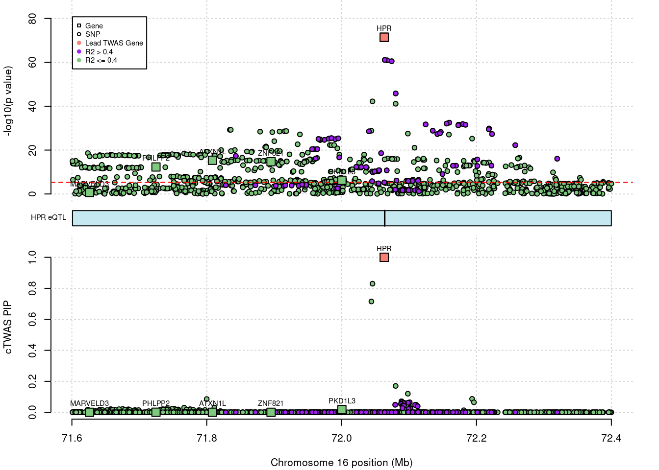
| Version | Author | Date |
|---|---|---|
| a764e3d | wesleycrouse | 2023-08-31 |
This plot function has an option include an empty space to add a gene
track (empty_gene_track=T); however, the gene track must be
plotted separately and manually aligned due to plotting
incompatibilities between base R and the Gviz package. Here
is an example that generates both the locus plot and the gene track,
with the plot sizes that we used in the paper to manually align the
plots.
NOTE: This is a pretty annoying limitation
and makes the plotting not entirely reproducible. I spent a lot of time
trying to get these plots to play nicely together but couldn’t make it
work. Basically, I couldn’t figure out how to get Gviz to respect the
plot panels in base R. Remaking the rest of the panels in
Gviz is an option, but by default, it doesn’t allow
different marker shapes (i.e. squares for genes and circles for SNPs) in
the same track.
#locus plot with empty space at the bottom for the gene track
pdf(file = paste0(outputdir, "HPR_locus_plot.pdf"), width = 5, height = 3.5)
plot_df <- ctwas_locus_plot(ctwas_res = ctwas_res,
                            region_tag = "16_1",
                            xlim = c(71.6,72.4),
                            ymax_twas = 85,
                            twas_sig_thresh = twas_sig_thresh,
                            alt_names = "genename",
                            legend_panel = "TWAS",
                            legend_side="left",
                            outputdir = outputdir,
                            outname = outname,
                            return_table = T,
                            empty_gene_track = T)
dev.off()

#gene track for the locus plot
pdf(file = paste0(outputdir, "HPR_locus_plot_genetrack.pdf"), width = 3.86, height = 0.6)
ctwas_locus_plot_genetrack(plot_df)
dev.off()
Running cTWAS genome-wide
We now provide a workflow for the same analysis, but using the full data and estimating parameters. This can be computationally intensive. We performed these analyses with 10 cores and 56GB of RAM, although the exact resource requirements will vary with the numbers of genes and variants provided.
Imputing gene z-scores
To impute gene z-scores genome-wide, we specify the full set of GWAS
summary statistics, the full PredictDB liver weights, and the full set
of LD reference matrices. This step can be slow, especially with both of
the advanced harmonization options turned on. There is a parallelized
version of this function in the multigroup branch of cTWAS.
As specified here, imputation took approximately 6 hours, using a single
core (the only option using the main branch). When getting
started with your own data, it may be helpful to run
impute_expr_z with both
recover_strand_ambig_wgt = F and
strand_ambig_action_z = "none" to make sure everything runs
correctly, before turning on these features for the final analysis.
NOTE: The parallelized version of this
function has some memory issues when
recover_strand_ambig_wgt = T and multiple cores are used.
This needs to be fixed by dividing up the covariances provided by
PredictDB into chunks, storing them, and then loading specific groups by
core. Currently, all the covariances are made available to every
core.
NOTE: How long does this take with
recover_strand_ambig_wgt = F? With
strand_ambig_action_z = "recover"? It take about 4.5 hours
with recovering weights turned off.
outputdir <- "results/whole_genome/"
outname <- "example_genome"

ld_R_dir <- "/project2/mstephens/wcrouse/UKB_LDR_0.1/"

dir.create(outputdir, showWarnings=F, recursive=T)

# get gene z score
if (file.exists(paste0(outputdir, outname, "_z_gene.Rd"))){
  ld_exprfs <- paste0(outputdir, outname, "_chr", 1:22, ".expr.gz")
  load(file = paste0(outputdir, outname, "_z_gene.Rd"))
  load(file = paste0(outputdir, outname, "_z_snp.Rd"))
} else {
  res <- impute_expr_z(z_snp = z_snp,
                     weight = weight,
                     ld_R_dir = ld_R_dir,
                     outputdir = outputdir,
                     outname = outname,
                     harmonize_z = T,
                     harmonize_wgt = T,
                     strand_ambig_action_z = "none",
                     recover_strand_ambig_wgt = T)

  z_gene <- res$z_gene
  ld_exprfs <- res$ld_exprfs
  z_snp <- res$z_snp

  save(z_gene, file = paste0(outputdir, outname, "_z_gene.Rd"))
  save(ld_exprfs, file = paste0(outputdir, outname, "_ld_exprfs.Rd"))
  save(z_snp, file = paste0(outputdir, outname, "_z_snp.Rd"))
}
Estimating parameters and fine-mapping
Now that we’ve imputed gene z-scores for the full genome, we are ready to run the full cTWAS analysis. The full analysis involves first estimating parameters from the data, and then fine-mapping the genes and variants using these estimated parameters.
As mentioned previously, the full cTWAS analysis can computationally
expensive, so we will specify several options to make the analysis
faster. The thin argument randomly selects 10% of variants
to use during the parameter estimation and initial fine-mapping steps,
reducing computation. The max_snp_region sets a maximum on
the number of variants that can be in a single (merged) region to
prevent memory issues during fine-mapping. The ncore
argument specifies the number of cores to use when parallelizing over
regions.
thin <- 0.1
max_snp_region <- 20000
ncore <- 6
We pass these arguments the ctwas_rss and run the full
analysis. As specified, using 6 cores and with 56GB of RAM available,
this step took approximately 7 hours.
# run ctwas_rss
ctwas_rss(z_gene = z_gene,
          z_snp = z_snp,
          ld_exprfs = ld_exprfs,
          ld_R_dir = ld_R_dir,
          ld_regions = "EUR",
          ld_regions_version = "b38",
          outputdir = outputdir,
          outname = outname,
          thin = thin,
          max_snp_region = max_snp_region,
          ncore = ncore)
The files in the output directory are similar to the single locus
example, but there are several additional files since we’ve performed
parameter estimation. Parameter estimation involves two steps. The first
step obtains a rough estimate for the parameters. These estimates are
saved in the *.s1.susieIrssres.Rd file. The SuSiE output
from the last iteration in this step is saved in
*.s1.susieIrss.txt; this file contains the total number of
variants analyzed by cTWAS, as used in PVE estimation, scaled by
thin. The second step obtains a more precise estimate for
the parameters using a subset of regions. These estimates are saved in
the *.s2.susieIrssres.Rd file; the final entry of this file
is the estimated parameters, scaled by the thin parameter.
The *.s2.susieIrss.txt file contains the SuSiE output from
the final iteration of this step.
After parameter estimation, cTWAS performs a first pass at
fine-mapping, using the proportion of variants specified in
thin. These results are saved in the
*.s3.susieIrss.txt. If thin is specified, then
for regions with a gene having PIP greater than
rerun_gene_PIP, cTWAS will make a final pass, analyzing
these regions using the full set of variants. The final output of cTWAS
is *.susieIrss.txt; this file contains results for all
genes, all variants in regions with strong gene signals, and 10% of
variants in other regions.
Assessing parameter estimates
We provide code to assess the convergence of the estimated parameters and to compute the proportion of variance explained (PVE) by variants and genes.
ctwas_parameters <- ctwas_summarize_parameters(outputdir = outputdir,
                                               outname = outname,
                                               gwas_n = gwas_n,
                                               thin = thin)

#number of variants in the analysis
ctwas_parameters$n_snps
[1] 8696600#number of genes in the analysis
ctwas_parameters$n_genes[1] 9881#estimated prior inclusion probability
ctwas_parameters$group_prior gene SNP
0.0107220302 0.0001715896 #estimated prior effect size
ctwas_parameters$group_prior_var gene SNP
41.327666 9.977841 #estimated enrichment of genes over variants
ctwas_parameters$enrichment[1] 62.48649#PVE explained by genes and variants
ctwas_parameters$group_pve gene SNP
0.01274204 0.04333086 #total heritability (sum of PVE)
ctwas_parameters$total_pve[1] 0.0560729#attributable heritability
ctwas_parameters$attributable_pve gene SNP
0.2272407 0.7727593 #plot convergence
ctwas_parameters$convergence_plot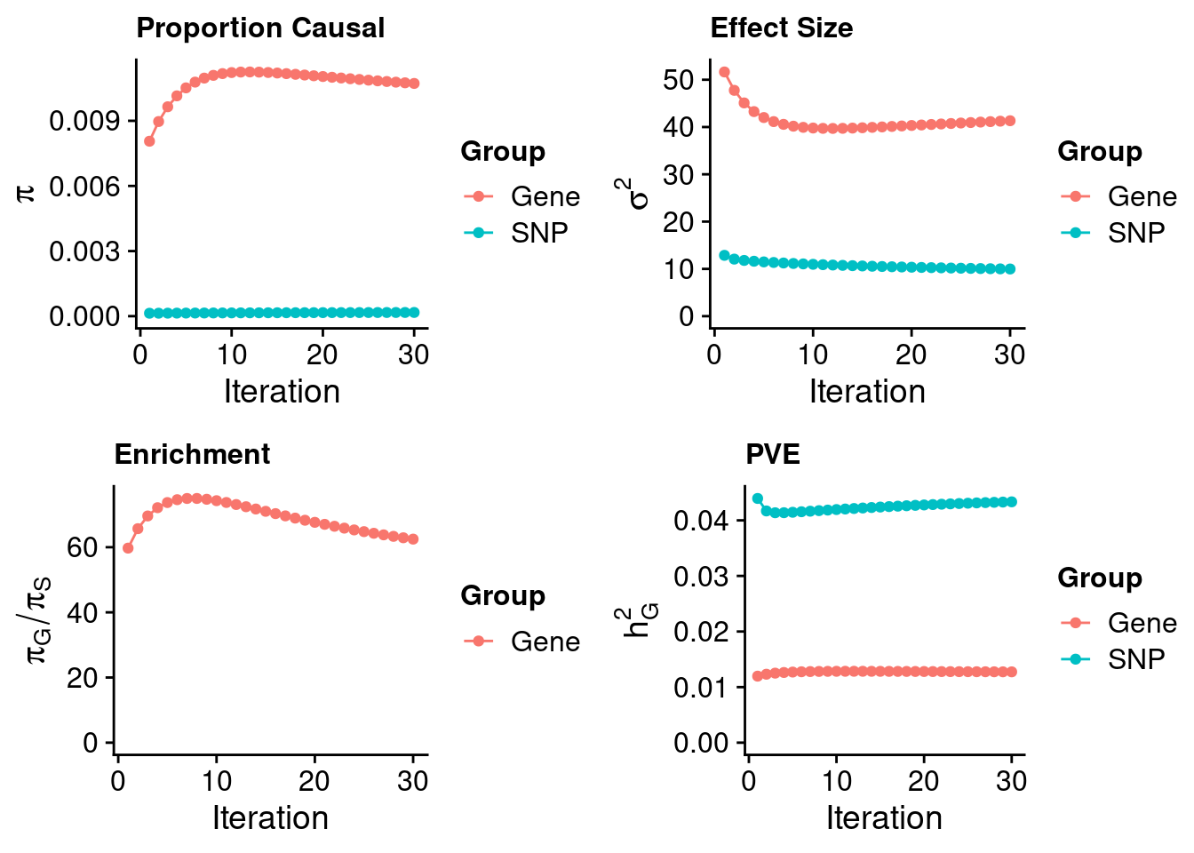
| Version | Author | Date |
|---|---|---|
| a764e3d | wesleycrouse | 2023-08-31 |
Viewing the results
As before, we will add the gene names to the results (the PredictDB weights use Ensembl IDs as the primary identifier), as well as the z-scores for each SNP and gene. We then show all genes with PIP greater than 0.8, which is the threshold we used in the paper.
#load cTWAS results
ctwas_res <- read.table(paste0(outputdir, outname, ".susieIrss.txt"), header=T)

#load gene information from PredictDB
sqlite <- RSQLite::dbDriver("SQLite")
db = RSQLite::dbConnect(sqlite, weight)
query <- function(...) RSQLite::dbGetQuery(db, ...)
gene_info <- query("select gene, genename, gene_type from extra")
RSQLite::dbDisconnect(db)

#add gene names to cTWAS results
ctwas_res$genename[ctwas_res$type=="gene"] <- gene_info$genename[match(ctwas_res$id[ctwas_res$type=="gene"], gene_info$gene)]

#add z-scores to cTWAS results
ctwas_res$z[ctwas_res$type=="SNP"] <- z_snp$z[match(ctwas_res$id[ctwas_res$type=="SNP"], z_snp$id)]
ctwas_res$z[ctwas_res$type=="gene"] <- z_gene$z[match(ctwas_res$id[ctwas_res$type=="gene"], z_gene$id)]

#display the genes with PIP > 0.8
ctwas_res <- ctwas_res[order(-ctwas_res$susie_pip),]
ctwas_res[ctwas_res$type=="gene" & ctwas_res$susie_pip > 0.8,]
chrom id pos type region_tag1 region_tag2
879255 1 ENSG00000134222.16 109275684 gene 1 67
1064449 16 ENSG00000261701.6 72063820 gene 16 38
913684 2 ENSG00000125629.14 118088372 gene 2 69
910002 2 ENSG00000143921.6 43839108 gene 2 27
1027995 11 ENSG00000149485.18 61829161 gene 11 34
957882 6 ENSG00000204599.14 30324306 gene 6 24
999614 9 ENSG00000165029.15 104906792 gene 9 53
990822 8 ENSG00000173273.15 9315699 gene 8 12
1049636 13 ENSG00000183087.14 113849020 gene 13 62
1111836 20 ENSG00000100979.14 45906012 gene 20 28
1096890 19 ENSG00000105287.12 46713856 gene 19 33
923078 2 ENSG00000163083.5 120552693 gene 2 70
894050 1 ENSG00000143771.11 224356827 gene 1 114
967636 7 ENSG00000105866.13 21553355 gene 7 19
950469 5 ENSG00000151292.17 123513182 gene 5 75
1093233 19 ENSG00000255974.7 40847202 gene 19 28
1096921 19 ENSG00000176920.11 48700572 gene 19 33
1088486 18 ENSG00000119537.15 63367187 gene 18 35
977014 7 ENSG00000015520.14 44541277 gene 7 32
977015 7 ENSG00000136271.10 44575121 gene 7 32
992988 9 ENSG00000155158.20 15280189 gene 9 13
987201 7 ENSG00000087087.18 100875204 gene 7 62
1005378 9 ENSG00000160447.6 128703202 gene 9 66
1010141 10 ENSG00000119965.12 122945179 gene 10 77
938455 5 ENSG00000152684.10 52787392 gene 5 31
1084624 17 ENSG00000173757.9 42276835 gene 17 25
928668 2 ENSG00000123612.15 157625480 gene 2 94
867597 1 ENSG00000162607.12 62436136 gene 1 39
852390 1 ENSG00000179023.8 18480845 gene 1 13
1017410 11 ENSG00000177685.16 827713 gene 11 1
1021453 11 ENSG00000179119.14 18634724 gene 11 13
987196 7 ENSG00000172336.4 100705751 gene 7 62
861235 1 ENSG00000142765.17 27342119 gene 1 19
901554 2 ENSG00000151360.9 3594771 gene 2 2
1042437 12 ENSG00000118971.7 4275678 gene 12 4
cs_index susie_pip mu2 genename z
879255 1 1.0000000 1667.48423 PSRC1 -41.687336
1064449 1 0.9999997 162.98924 HPR -17.962770
913684 1 0.9999957 68.37263 INSIG2 -8.982702
910002 1 0.9999453 312.10767 ABCG8 -20.293982
1027995 1 0.9998404 163.46291 FADS1 12.926351
957882 1 0.9985885 71.89752 TRIM39 8.840164
999614 4 0.9955314 70.13575 ABCA1 7.982017
990822 1 0.9910883 76.13390 TNKS 11.038564
1049636 1 0.9883382 71.11508 GAS6 -8.923688
1111836 2 0.9883283 61.28528 PLTP -5.732491
1096890 2 0.9871587 29.99928 PRKD2 5.072217
923078 1 0.9825109 73.79864 INHBB -8.518936
894050 1 0.9789702 40.69262 CNIH4 6.145535
967636 1 0.9759456 101.98305 SP4 10.693191
950469 1 0.9745191 83.85862 CSNK1G3 9.116291
1093233 1 0.9650551 31.87939 CYP2A6 5.407028
1096921 1 0.9641649 104.43211 FUT2 -11.927107
1088486 1 0.9602264 24.59603 KDSR -4.526287
977014 1 0.9515004 86.82732 NPC1L1 -10.761931
977015 2 0.9495892 59.83144 DDX56 9.641861
992988 0 0.9450026 23.14602 TTC39B -4.334495
987201 2 0.9405116 32.60063 SRRT 5.424996
1005378 1 0.9380390 47.46054 PKN3 -6.620563
1010141 1 0.9371487 37.07672 C10orf88 -6.787850
938455 1 0.9363014 70.56030 PELO 8.288398
1084624 1 0.9336311 30.56463 STAT5B 5.426252
928668 0 0.9320372 25.78698 ACVR1C -4.687370
867597 1 0.8941255 252.81074 USP1 16.258211
852390 0 0.8393363 22.17420 KLHDC7A 4.124187
1017410 0 0.8274447 21.52123 CRACR2B -3.989585
1021453 1 0.8251281 33.41511 SPTY2D1 -5.557123
987196 3 0.8234854 40.37437 POP7 -5.845258
861235 0 0.8163154 22.15199 SYTL1 -3.962854
901554 1 0.8133753 28.04053 ALLC 4.919066
1042437 0 0.8041948 22.63603 CCND2 -4.065830We will also visualize the POLK locus that we highlighted in the
paper. As mentioned previously, the cTWAS output includes results for
all genes, but it only includes a fraction of variants if the
thin parameter is specified. There are complete variant
results in regions with gene PIP greater than
rerun_gene_PIP, but there are incomplete variant results in
regions with weaker gene signals. The POLK locus is a “null” result;
after running cTWAS, there is no strong gene signal. Thus, in order to
plot the full set of variants at this locus, we must specify
rerun_ctwas=T to run cTWAS again at this locus using all
variants. This calls ctwas_rss and logs its progress; it
also create a temporary folder within the output directory to store the
results. After doing this the first time, you can set
rerun_load_only=T to make changes to the plot without
calling cTWAS again.
#genome-wide bonferroni threshold used for TWAS
twas_sig_thresh <- 0.05/sum(ctwas_res$type=="gene")

#show cTWAS result for POLK and store region_tag
ctwas_res[which(ctwas_res$genename=="POLK"),]
chrom id pos type region_tag1 region_tag2 cs_index
281171 5 ENSG00000122008.15 75510279 gene 5 45 0
susie_pip mu2 genename z
281171 0.004653312 218.9507 POLK 17.51576region_tag <- "5_45"
#plot the POLK locus
ctwas_locus_plot(ctwas_res = ctwas_res,
region_tag = region_tag,
xlim = c(75,75.8),
twas_sig_thresh = twas_sig_thresh,
alt_names = "genename",
legend_panel = "cTWAS",
legend_side = "left",
outputdir = outputdir,
outname = outname,
rerun_ctwas = T,
z_snp = z_snp,
z_gene = z_gene)2023-09-12 11:30:24 INFO::ctwas started ...
2023-09-12 11:30:46 INFO::LD region file: results/whole_genome/temp_plot/temp_reg.bed
2023-09-12 11:30:46 INFO::No. LD regions: 1
2023-09-12 11:30:49 INFO::No. regions with at least one SNP/gene for chr1: 0
2023-09-12 11:30:49 INFO::No. regions with at least one SNP/gene for chr1 after merging: 0
2023-09-12 11:30:50 INFO::No. regions with at least one SNP/gene for chr2: 0
2023-09-12 11:30:50 INFO::No. regions with at least one SNP/gene for chr2 after merging: 0
2023-09-12 11:30:50 INFO::No. regions with at least one SNP/gene for chr3: 0
2023-09-12 11:30:50 INFO::No. regions with at least one SNP/gene for chr3 after merging: 0
2023-09-12 11:30:52 INFO::No. regions with at least one SNP/gene for chr4: 0
2023-09-12 11:30:52 INFO::No. regions with at least one SNP/gene for chr4 after merging: 0
2023-09-12 11:30:52 INFO::No. regions with at least one SNP/gene for chr5: 1
2023-09-12 11:30:52 INFO::No. regions with at least one SNP/gene for chr5 after merging: 1
2023-09-12 11:30:53 INFO::No. regions with at least one SNP/gene for chr6: 0
2023-09-12 11:30:53 INFO::No. regions with at least one SNP/gene for chr6 after merging: 0
2023-09-12 11:30:53 INFO::No. regions with at least one SNP/gene for chr7: 0
2023-09-12 11:30:53 INFO::No. regions with at least one SNP/gene for chr7 after merging: 0
2023-09-12 11:30:54 INFO::No. regions with at least one SNP/gene for chr8: 0
2023-09-12 11:30:54 INFO::No. regions with at least one SNP/gene for chr8 after merging: 0
2023-09-12 11:30:54 INFO::No. regions with at least one SNP/gene for chr9: 0
2023-09-12 11:30:55 INFO::No. regions with at least one SNP/gene for chr9 after merging: 0
2023-09-12 11:30:55 INFO::No. regions with at least one SNP/gene for chr10: 0
2023-09-12 11:30:55 INFO::No. regions with at least one SNP/gene for chr10 after merging: 0
2023-09-12 11:30:55 INFO::No. regions with at least one SNP/gene for chr11: 0
2023-09-12 11:30:55 INFO::No. regions with at least one SNP/gene for chr11 after merging: 0
2023-09-12 11:30:56 INFO::No. regions with at least one SNP/gene for chr12: 0
2023-09-12 11:30:56 INFO::No. regions with at least one SNP/gene for chr12 after merging: 0
2023-09-12 11:30:56 INFO::No. regions with at least one SNP/gene for chr13: 0
2023-09-12 11:30:56 INFO::No. regions with at least one SNP/gene for chr13 after merging: 0
2023-09-12 11:30:57 INFO::No. regions with at least one SNP/gene for chr14: 0
2023-09-12 11:30:57 INFO::No. regions with at least one SNP/gene for chr14 after merging: 0
2023-09-12 11:30:57 INFO::No. regions with at least one SNP/gene for chr15: 0
2023-09-12 11:30:57 INFO::No. regions with at least one SNP/gene for chr15 after merging: 0
2023-09-12 11:30:57 INFO::No. regions with at least one SNP/gene for chr16: 0
2023-09-12 11:30:57 INFO::No. regions with at least one SNP/gene for chr16 after merging: 0
2023-09-12 11:30:57 INFO::No. regions with at least one SNP/gene for chr17: 0
2023-09-12 11:30:57 INFO::No. regions with at least one SNP/gene for chr17 after merging: 0
2023-09-12 11:30:58 INFO::No. regions with at least one SNP/gene for chr18: 0
2023-09-12 11:30:58 INFO::No. regions with at least one SNP/gene for chr18 after merging: 0
2023-09-12 11:30:58 INFO::No. regions with at least one SNP/gene for chr19: 0
2023-09-12 11:30:58 INFO::No. regions with at least one SNP/gene for chr19 after merging: 0
2023-09-12 11:30:58 INFO::No. regions with at least one SNP/gene for chr20: 0
2023-09-12 11:30:58 INFO::No. regions with at least one SNP/gene for chr20 after merging: 0
2023-09-12 11:30:58 INFO::No. regions with at least one SNP/gene for chr21: 0
2023-09-12 11:30:58 INFO::No. regions with at least one SNP/gene for chr21 after merging: 0
2023-09-12 11:30:59 INFO::No. regions with at least one SNP/gene for chr22: 0
2023-09-12 11:30:59 INFO::No. regions with at least one SNP/gene for chr22 after merging: 0
2023-09-12 11:30:59 INFO::Trim regions with SNPs more than Inf
2023-09-12 11:30:59 INFO::Adding R matrix info, as genotype is not given
2023-09-12 11:30:59 INFO::Adding R matrix info for chrom 1
2023-09-12 11:30:59 INFO::Adding R matrix info for chrom 2
2023-09-12 11:30:59 INFO::Adding R matrix info for chrom 3
2023-09-12 11:30:59 INFO::Adding R matrix info for chrom 4
2023-09-12 11:30:59 INFO::Adding R matrix info for chrom 5Warning in asMethod(object): sparse->dense coercion: allocating vector of size
1.3 GiB2023-09-12 11:31:36 INFO::Adding R matrix info for chrom 6
2023-09-12 11:31:36 INFO::Adding R matrix info for chrom 7
2023-09-12 11:31:36 INFO::Adding R matrix info for chrom 8
2023-09-12 11:31:36 INFO::Adding R matrix info for chrom 9
2023-09-12 11:31:36 INFO::Adding R matrix info for chrom 10
2023-09-12 11:31:36 INFO::Adding R matrix info for chrom 11
2023-09-12 11:31:36 INFO::Adding R matrix info for chrom 12
2023-09-12 11:31:36 INFO::Adding R matrix info for chrom 13
2023-09-12 11:31:36 INFO::Adding R matrix info for chrom 14
2023-09-12 11:31:36 INFO::Adding R matrix info for chrom 15
2023-09-12 11:31:36 INFO::Adding R matrix info for chrom 16
2023-09-12 11:31:36 INFO::Adding R matrix info for chrom 17
2023-09-12 11:31:36 INFO::Adding R matrix info for chrom 18
2023-09-12 11:31:36 INFO::Adding R matrix info for chrom 19
2023-09-12 11:31:36 INFO::Adding R matrix info for chrom 20
2023-09-12 11:31:36 INFO::Adding R matrix info for chrom 21
2023-09-12 11:31:36 INFO::Adding R matrix info for chrom 22
2023-09-12 11:31:36 INFO::Run susie for all regions.
2023-09-12 11:31:36 INFO::run iteration 1Warning in asMethod(object): sparse->dense coercion: allocating vector of size
1.3 GiB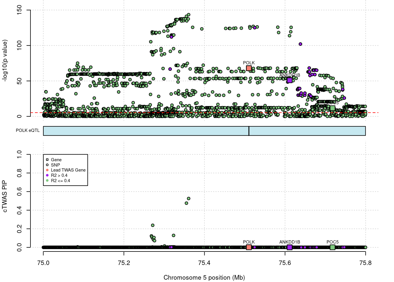
| Version | Author | Date |
|---|---|---|
| a764e3d | wesleycrouse | 2023-08-31 |
Cleaning up
The summary statistics version of cTWAS generates a lot of files.
cTWAS added variant-by-gene and gene-by-gene correlation information (“R
matrix info”) for all regions in a directory called
[outname]_LDR, and it also stored thinned version of the LD
matrices in the same directory. We store all these files to speed
computation, and we leave them unzipped at the end of the analysis so
that they can be used with ctwas_locus_plot. However, once
you are done with an analysis, we recommend zipping the contents of the
[outname]_LDR folder.
system(paste0("tar -zcvf ", outputdir, outname, "_LDR.tar.gz ", outputdir, outname, "_LDR"))
system(paste0("rm -r ", outputdir, outname, "_LDR"))
NOTE: Is it possible to zip the results and access only what you need within the locus plot function?
Other Topics
Harmonization
The input data for cTWAS must be harmonized prior to analysis (i.e. the reference and alternative alleles for each variant should match across all three data sources). We provide some options for harmonization during the gene imputation step if the data are not already harmonized. These options separately harmonizing the GWAS summary statistics and the prediction models to the LD reference. The full harmonization procedures are described in the methods section of the paper. Here, we will provide a quick description of how harmonization works, and when it should be used.
If harmonization is off, cTWAS will use the union of variants in the GWAS reference, the prediction models, and the LD reference for imputation, and it will use the z-score and weights as-is.
For the GWAS summary statistics and the prediction models, there are
two options that turn on “simple” harmonization:
harmonize_z = T and harmonize_wgt = T. Simple
harmonization flips reference and alternate alleles to match the LD
reference. This procedure is fast, and for variants that are not strand
ambiguous, this is all that is required for harmonization. However,
strand ambiguous variants (A<->T and C<->G substitutions)
are not necessarily harmonized, as the strand used to determine the
ref/alt alleles could be different between different datasets, and this
is indistinguishable from a ref/alt allele swap. Turning on
harmonization requires making a decision about how to handle these
strand ambiguous variants.
For the z-scores, there are three options for strand ambiguous
variants, specified by strand_ambig_action_z. The
"drop" option removes strand ambiguous variants; the
"none" option takes no action, effectively treating strand
ambiguous variants as unambiguous; and the "recover" option
uses the imputation-based procedure described in the paper to recover
strand ambiguous variants. The “recover” option can be computationally
expensive.
For the weights, there are two options for strand ambiguous variants,
specified by recover_strand_ambig_wgt. Setting this equal
to FALSE removes strand ambiguous variants; setting it to
TRUE will use the LD-based procedure described in the paper
to recover strand ambiguous weights. This recovery procedure does
increase runtime, but it is less expensive than the recovery procedure
for the z-scores.
NOTE: Need to add option to take no action on strand ambiguous weights when harmonization is turned on.
In the paper and in this document, because the z-scores and the LD
reference were from the same source (UK Biobank), we expect that the
strand is consistent between the GWAS and LD reference, so we used the
option strand_ambig_action_z = "none" to treat strand
ambiguous variants as unambiguous. The prediction models are from a
different population (GTEx), so for strand ambiguous variants in the
prediction models, we used recover_strand_ambig_wgt=T.
Note that we include a function to pre-harmonize the GWAS summary
statistics: preharmonize_z_ld. If using this function at
the start of the analysis, you can set harmonize_z = F
during imputation.
Region Merging
cTWAS performs its analysis region-by-region in order to make the
analysis tractable. By default, regions are merged
(merge=T) and analyzed jointly when a gene spans a region
boundary; this ensures that these genes are analyzed in their
appropriate context, which includes information from both regions. Gene
start and end positions are determined by the first and last variant
positions for each gene prediction model, for variants that are also in
the LD reference and GWAS summary statistics. Thus, the actual regions
analyzed by cTWAS depend not only on the specified region locations, but
also the LD and summary statistics supplied. Region definitions are
data-dependent in this way.
cTWAS is region-based for computational reasons, so it follows that excessive region merging (i.e. combining many adjacent regions) can make the analysis slow or intractable. This is especially true if there are already many variants in the LD reference. The cTWAS log reports the number of regions on each chromosome before and after merging. If more than a handful of regions are merged, there many be computational issues in subsequent steps, or something many misspecified. There are at least two scenarios that can lead to excessive region merging.
First, it is possible that the specified prediction models are dense (they contain many variants per gene), or that they span a large genomic region. This can result in many boundary-spanning genes and many merged regions. For this reason, cTWAS performs best when prediction models are sparse. If using dense prediction models, we recommend removing variants with weight below a threshold from the prediction models prior to analysis. We also recommend prediction models that only use variants nearby the gene for the same reason.
Second, mismatching the genome build (e.g. hg38) of the LD reference and the genome build used to train the prediction models can lead to excessive region merging. If the genome builds are mismatched, it is possible that variants included in a prediction model for a gene are not near the gene in the LD reference. Such a gene could potentially span many region boundaries. It is critical that the genome build of the LD reference match the genome build used to train the prediction models. The genome build of the GWAS summary statistics does not matter because variant positions are determined by the LD reference.
Turning region merging off (merge=F) discards all genes
that span region boundaries. This will resolve computational issues
around excessive region merging but will also prevent the analysis of
boundary-spanning genes.
sessionInfo()R version 4.1.0 (2021-05-18)
Platform: x86_64-pc-linux-gnu (64-bit)
Running under: CentOS Linux 7 (Core)
Matrix products: default
BLAS: /software/R-4.1.0-no-openblas-el7-x86_64/lib64/R/lib/libRblas.so
LAPACK: /software/R-4.1.0-no-openblas-el7-x86_64/lib64/R/lib/libRlapack.so
locale:
[1] LC_CTYPE=en_US.UTF-8 LC_NUMERIC=C LC_TIME=C
[4] LC_COLLATE=C LC_MONETARY=C LC_MESSAGES=C
[7] LC_PAPER=C LC_NAME=C LC_ADDRESS=C
[10] LC_TELEPHONE=C LC_MEASUREMENT=C LC_IDENTIFICATION=C
attached base packages:
[1] stats graphics grDevices utils datasets methods base
other attached packages:
[1] cowplot_1.1.1 ggplot2_3.4.0 RSQLite_2.3.1 ctwas_0.1.35
[5] workflowr_1.7.0
loaded via a namespace (and not attached):
[1] Rcpp_1.0.11 lattice_0.20-45 getPass_0.2-2 ps_1.7.2
[5] assertthat_0.2.1 rprojroot_2.0.3 digest_0.6.31 foreach_1.5.2
[9] utf8_1.2.3 R6_2.5.1 evaluate_0.18 httr_1.4.4
[13] highr_0.9 pillar_1.9.0 rlang_1.1.1 rstudioapi_0.14
[17] data.table_1.14.8 whisker_0.4.1 callr_3.7.3 jquerylib_0.1.4
[21] blob_1.2.4 Matrix_1.5-3 rmarkdown_2.18 labeling_0.4.2
[25] readr_2.1.4 stringr_1.5.0 bit_4.0.5 munsell_0.5.0
[29] compiler_4.1.0 httpuv_1.6.6 xfun_0.35 pkgconfig_2.0.3
[33] htmltools_0.5.4 tidyselect_1.2.0 tibble_3.2.1 logging_0.10-108
[37] codetools_0.2-18 fansi_1.0.4 withr_2.5.0 crayon_1.5.2
[41] dplyr_1.0.10 tzdb_0.4.0 later_1.3.0 grid_4.1.0
[45] jsonlite_1.8.4 gtable_0.3.1 lifecycle_1.0.3 DBI_1.1.3
[49] git2r_0.30.1 magrittr_2.0.3 scales_1.2.1 cli_3.6.1
[53] stringi_1.7.8 cachem_1.0.8 farver_2.1.1 fs_1.5.2
[57] promises_1.2.0.1 doParallel_1.0.17 pgenlibr_0.3.6 bslib_0.4.1
[61] generics_0.1.3 vctrs_0.6.3 iterators_1.0.14 tools_4.1.0
[65] bit64_4.0.5 glue_1.6.2 hms_1.1.3 processx_3.8.0
[69] parallel_4.1.0 fastmap_1.1.1 yaml_2.3.6 colorspace_2.0-3
[73] memoise_2.0.1 knitr_1.41 sass_0.4.4