Testing Variance Prior for cTWAS
wesleycrouse
2023-06-26
Last updated: 2023-08-18
Checks: 6 1
Knit directory: ctwas_applied/
This reproducible R Markdown analysis was created with workflowr (version 1.7.0). The Checks tab describes the reproducibility checks that were applied when the results were created. The Past versions tab lists the development history.
The R Markdown file has unstaged changes. To know which version of
the R Markdown file created these results, you’ll want to first commit
it to the Git repo. If you’re still working on the analysis, you can
ignore this warning. When you’re finished, you can run
wflow_publish to commit the R Markdown file and build the
HTML.
Great job! The global environment was empty. Objects defined in the global environment can affect the analysis in your R Markdown file in unknown ways. For reproduciblity it’s best to always run the code in an empty environment.
The command set.seed(20210726) was run prior to running
the code in the R Markdown file. Setting a seed ensures that any results
that rely on randomness, e.g. subsampling or permutations, are
reproducible.
Great job! Recording the operating system, R version, and package versions is critical for reproducibility.
Nice! There were no cached chunks for this analysis, so you can be confident that you successfully produced the results during this run.
Great job! Using relative paths to the files within your workflowr project makes it easier to run your code on other machines.
Great! You are using Git for version control. Tracking code development and connecting the code version to the results is critical for reproducibility.
The results in this page were generated with repository version ce02b6f. See the Past versions tab to see a history of the changes made to the R Markdown and HTML files.
Note that you need to be careful to ensure that all relevant files for
the analysis have been committed to Git prior to generating the results
(you can use wflow_publish or
wflow_git_commit). workflowr only checks the R Markdown
file, but you know if there are other scripts or data files that it
depends on. Below is the status of the Git repository when the results
were generated:
Untracked files:
    Untracked:  gwas.RData
    Untracked:  ld_R_info.RData
    Untracked:  z_snp_pos_ebi-a-GCST004131.RData
    Untracked:  z_snp_pos_ebi-a-GCST004132.RData
    Untracked:  z_snp_pos_ebi-a-GCST004133.RData
    Untracked:  z_snp_pos_scz-2018.RData
    Untracked:  z_snp_pos_ukb-a-360.RData
    Untracked:  z_snp_pos_ukb-d-30780_irnt.RData

Unstaged changes:
    Modified:   analysis/variance_prior_testing.Rmd
Note that any generated files, e.g. HTML, png, CSS, etc., are not included in this status report because it is ok for generated content to have uncommitted changes.
These are the previous versions of the repository in which changes were
made to the R Markdown
(analysis/variance_prior_testing.Rmd) and HTML
(docs/variance_prior_testing.html) files. If you’ve
configured a remote Git repository (see ?wflow_git_remote),
click on the hyperlinks in the table below to view the files as they
were in that past version.
| File | Version | Author | Date | Message |
|---|---|---|---|---|
| html | ce02b6f | wesleycrouse | 2023-08-18 | fixing variance prior report |
| Rmd | 1632c6b | wesleycrouse | 2023-07-27 | fixing gamma prior results |
| Rmd | 05b0117 | wesleycrouse | 2023-07-27 | adding results for inv-gamma prior on variance |
analysis_id <- "ukb-d-30660_irnt_Liver"
trait_id <- "ukb-d-30660_irnt"

source("/project2/mstephens/wcrouse/ctwas_multigroup_testing/ctwas_config.R")
E-M with Inverse-Gamma Prior on Variance
Likelihood Function
The complete log likelihood for a single group. For completeness, [brackets] denote variables that are conditionally independent.
Dropping conditionally independent variables from the notation:
Gamma prior on the precision
Hyperparameter \(a\) is the shape and \(b\) is the rate.
\(\sigma^{-2} \sim \mathrm{Gamma}(a,b)\)
\(\mathrm{logp}(\sigma^{-2}) = a\mathrm{log}(b) - \mathrm{log}(\Gamma(a)) + (a-1)\mathrm{log}(\sigma^{-2}) -b\sigma^{-2}\)
E-M update for the variance
Take the expectation over \(\beta,\Gamma|\pi^{t},\sigma^{t}\), then take the derivative with respect to \(\sigma^{-2}\) and set it equal to zero. \(\alpha_{j}\) is the PIP of variable \(j\).
\((\sigma^{2})^{t+1} = \frac{0.5\sum_{j}[\alpha_{j}\tau_{j}]+b}{0.5\sum[\alpha_j] + a - 1}\)
Case 31 - Bilirubin with Liver - Independent Variance
Load ctwas results
results_dir <- paste0("/project2/mstephens/wcrouse/ctwas_multigroup_testing/ukb-d-30780_irnt/multigroup_case31")

weight <- "/project2/compbio/predictdb/mashr_models/mashr_Liver.db"

#load information for all genes

gene_info <- data.frame(gene=as.character(), genename=as.character(), gene_type=as.character(), weight=as.character())

for (i in 1:length(weight)){
  sqlite <- RSQLite::dbDriver("SQLite")
  db = RSQLite::dbConnect(sqlite, weight[i])
  query <- function(...) RSQLite::dbGetQuery(db, ...)
  gene_info_current <- query("select gene, genename, gene_type from extra")
  RSQLite::dbDisconnect(db)

  gene_info_current$weight <- weight[i]

  gene_info <- rbind(gene_info, gene_info_current)
}

gene_info$group <- sapply(1:nrow(gene_info), function(x){paste0(unlist(strsplit(tools::file_path_sans_ext(rev(unlist(strsplit(gene_info$weight[x], "/")))[1]), "_"))[-1], collapse="_")})

gene_info$gene_id <- paste(gene_info$gene, gene_info$group, sep="|")

# #load ctwas results
# ctwas_res <- data.table::fread(paste0(results_dir, "/", analysis_id, "_ctwas.susieIrss.txt"))
#
# #make unique identifier for regions
# ctwas_res$region_tag <- paste(ctwas_res$region_tag1, ctwas_res$region_tag2, sep="_")

#load z scores for SNPs and collect sample size
load(paste0(results_dir, "/", analysis_id, "_expr_z_snp.Rd"))

sample_size <- z_snp$ss
sample_size <- as.numeric(names(which.max(table(sample_size))))

# #compute PVE for each gene/SNP
# ctwas_res$PVE = ctwas_res$susie_pip*ctwas_res$mu2/sample_size
#
# #separate gene and SNP results
# ctwas_gene_res <- ctwas_res[ctwas_res$type != "SNP", ]
# ctwas_gene_res <- data.frame(ctwas_gene_res)
# ctwas_snp_res <- ctwas_res[ctwas_res$type == "SNP", ]
# ctwas_snp_res <- data.frame(ctwas_snp_res)
#
# #add gene information to results
# ctwas_gene_res$gene_id <- sapply(ctwas_gene_res$id, function(x){unlist(strsplit(x, split="[|]"))[1]})
# ctwas_gene_res$group <- ctwas_gene_res$type
# ctwas_gene_res$alt_name <- paste0(ctwas_gene_res$gene_id, "|", ctwas_gene_res$group)
#
# ctwas_gene_res$genename <- NA
# ctwas_gene_res$gene_type <- NA
#
# group_list <- unique(ctwas_gene_res$group)
#
# for (j in 1:length(group_list)){
#   print(j)
#   group <- group_list[j]
#
#   res_group_indx <- which(ctwas_gene_res$group==group)
#   gene_info_group <- gene_info[gene_info$group==group,,drop=F]
#
#   ctwas_gene_res[res_group_indx,c("genename", "gene_type")] <- gene_info_group[sapply(ctwas_gene_res$alt_name[res_group_indx], match, gene_info_group$gene_id), c("genename", "gene_type")]
# }

#add z scores to results
load(paste0(results_dir, "/", analysis_id, "_expr_z_gene.Rd"))
#ctwas_gene_res$z <- z_gene[ctwas_gene_res$id,]$z

#z_snp <- z_snp[z_snp$id %in% ctwas_snp_res$id,]
#ctwas_snp_res$z <- z_snp$z[match(ctwas_snp_res$id, z_snp$id)]

# #merge gene and snp results with added information
# ctwas_snp_res$gene_id=NA
# ctwas_snp_res$group="SNP"
# ctwas_snp_res$alt_name=NA
# ctwas_snp_res$genename=NA
# ctwas_snp_res$gene_type=NA
#
# ctwas_res <- rbind(ctwas_gene_res,
#                    ctwas_snp_res[,colnames(ctwas_gene_res)])

#get number of SNPs from s1 results; adjust for thin argument
ctwas_res_s1 <- data.table::fread(paste0(results_dir, "/", analysis_id, "_ctwas.s1.susieIrss.txt"))
n_snps <- sum(ctwas_res_s1$type=="SNP")/thin
rm(ctwas_res_s1)

# #store columns to report
# report_cols <- colnames(ctwas_gene_res)[!(colnames(ctwas_gene_res) %in% c("type", "region_tag1", "region_tag2", "cs_index", "gene_type", "z_flag", "id", "chrom", "pos", "alt_name", "gene_id"))]
# first_cols <- c("genename", "group", "region_tag")
# report_cols <- c(first_cols, report_cols[!(report_cols %in% first_cols)])
Check convergence of parameters
library(ggplot2)
library(cowplot)

load(paste0(results_dir, "/", analysis_id, "_ctwas.s2.susieIrssres.Rd"))

#estimated group prior (all iterations)
estimated_group_prior_all <- group_prior_rec
estimated_group_prior_all["SNP",] <- estimated_group_prior_all["SNP",]*thin #adjust parameter to account for thin argument

#estimated group prior variance (all iterations)
estimated_group_prior_var_all <- group_prior_var_rec

#set group size
group_size <- structure(c(n_snps, nrow(z_gene)), names=c("SNP","gene"))

#estimated group PVE (all iterations)
estimated_group_pve_all <- estimated_group_prior_var_all*estimated_group_prior_all*group_size/sample_size #check PVE calculation

#estimated enrichment of genes (all iterations)
estimated_enrichment_all <- t(sapply(rownames(estimated_group_prior_all)[rownames(estimated_group_prior_all)!="SNP"], function(x){estimated_group_prior_all[rownames(estimated_group_prior_all)==x,]/estimated_group_prior_all[rownames(estimated_group_prior_all)=="SNP"]}))

title_size <- 12

df <- data.frame(niter = rep(1:ncol(estimated_group_prior_all), nrow(estimated_group_prior_all)),
                 value = unlist(lapply(1:nrow(estimated_group_prior_all), function(x){estimated_group_prior_all[x,]})),
                 group = rep(rownames(estimated_group_prior_all), each=ncol(estimated_group_prior_all)))

groupnames_for_plots <- sapply(as.character(unique(df$group)), function(x){paste(sapply(unlist(strsplit(x, "_")), substr, start=1, stop=3), collapse="_")})

df$group <- groupnames_for_plots[df$group]
df$group <- as.factor(df$group)

p_pi <- ggplot(df, aes(x=niter, y=value, group=group)) +
  geom_line(aes(color=group)) +
  geom_point(aes(color=group)) +
  xlab("Iteration") + ylab(bquote(pi)) +
  ggtitle("Proportion Causal") +
  theme_cowplot()

p_pi <- p_pi + theme(plot.title=element_text(size=title_size)) +
  expand_limits(y=0) +
  guides(color = guide_legend(title = "Group")) + theme (legend.title = element_text(size=12, face="bold"))

df <- data.frame(niter = rep(1:ncol(estimated_group_prior_var_all), nrow(estimated_group_prior_var_all)),
                 value = unlist(lapply(1:nrow(estimated_group_prior_var_all), function(x){estimated_group_prior_var_all[x,]})),
                 group = rep(rownames(estimated_group_prior_var_all), each=ncol(estimated_group_prior_var_all)))

groupnames_for_plots <- sapply(as.character(unique(df$group)), function(x){paste(sapply(unlist(strsplit(x, "_")), substr, start=1, stop=3), collapse="_")})

df$group <- groupnames_for_plots[df$group]
df$group <- as.factor(df$group)

p_sigma2 <- ggplot(df, aes(x=niter, y=value, group=group)) +
  geom_line(aes(color=group)) +
  geom_point(aes(color=group)) +
  xlab("Iteration") + ylab(bquote(sigma^2)) +
  ggtitle("Effect Size") +
  theme_cowplot()

p_sigma2 <- p_sigma2 + theme(plot.title=element_text(size=title_size)) +
  expand_limits(y=0) +
  guides(color = guide_legend(title = "Group")) + theme (legend.title = element_text(size=12, face="bold"))

df <- data.frame(niter = rep(1:ncol(estimated_group_pve_all), nrow(estimated_group_pve_all)),
                 value = unlist(lapply(1:nrow(estimated_group_pve_all), function(x){estimated_group_pve_all[x,]})),
                 group = rep(rownames(estimated_group_pve_all), each=ncol(estimated_group_pve_all)))

groupnames_for_plots <- sapply(as.character(unique(df$group)), function(x){paste(sapply(unlist(strsplit(x, "_")), substr, start=1, stop=3), collapse="_")})

df$group <- groupnames_for_plots[df$group]
df$group <- as.factor(df$group)

p_pve <- ggplot(df, aes(x=niter, y=value, group=group)) +
  geom_line(aes(color=group)) +
  geom_point(aes(color=group)) +
  xlab("Iteration") + ylab(bquote(h^2[G])) +
  ggtitle("PVE") +
  theme_cowplot()

p_pve <- p_pve + theme(plot.title=element_text(size=title_size)) +
  expand_limits(y=0) +
  guides(color = guide_legend(title = "Group")) + theme (legend.title = element_text(size=12, face="bold"))

df <- data.frame(niter = rep(1:ncol(estimated_enrichment_all), nrow(estimated_enrichment_all)),
                 value = unlist(lapply(1:nrow(estimated_enrichment_all), function(x){estimated_enrichment_all[x,]})),
                 group = rep(rownames(estimated_enrichment_all), each=ncol(estimated_enrichment_all)))

groupnames_for_plots <- sapply(as.character(unique(df$group)), function(x){paste(sapply(unlist(strsplit(x, "_")), substr, start=1, stop=3), collapse="_")})

df$group <- groupnames_for_plots[df$group]
df$group <- as.factor(df$group)

p_enrich <- ggplot(df, aes(x=niter, y=value, group=group)) +
  geom_line(aes(color=group)) +
  geom_point(aes(color=group)) +
  xlab("Iteration") + ylab(bquote(pi[G]/pi[S])) +
  ggtitle("Enrichment") +
  theme_cowplot()

p_enrich <- p_enrich + theme(plot.title=element_text(size=title_size)) +
  expand_limits(y=0) +
  guides(color = guide_legend(title = "Group")) + theme (legend.title = element_text(size=12, face="bold"))

plot_grid(p_pi + theme(legend.position = "none"),
          p_sigma2 + theme(legend.position = "none"),
          p_enrich + theme(legend.position = "none"),
          p_pve+ theme(legend.position = "none"))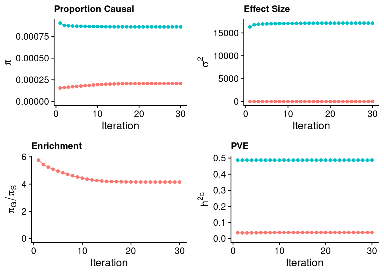
| Version | Author | Date |
|---|---|---|
| ce02b6f | wesleycrouse | 2023-08-18 |
#p_pi
#p_sigma2 + theme(legend.position = "none")
#p_enrich + theme(legend.position = "none")
#p_pve + theme(legend.position = "none")

####################

#estimated group prior
estimated_group_prior <- estimated_group_prior_all[,ncol(group_prior_rec)]
-sort(-estimated_group_prior)
gene SNP
0.0008594861 0.0002070674 #estimated group prior variance
estimated_group_prior_var <- estimated_group_prior_var_all[,ncol(group_prior_var_rec)]
-sort(-estimated_group_prior_var) gene SNP
17150.42864 6.14623 #estimated enrichment
estimated_enrichment <- estimated_enrichment_all[,ncol(group_prior_var_rec)]
-sort(-estimated_enrichment) gene
4.150755 #report sample size
print(sample_size)[1] 292933#report group size
print(group_size) SNP gene
8696600 9687 #estimated group PVE
estimated_group_pve <- estimated_group_pve_all[,ncol(group_prior_rec)]
-sort(-estimated_group_pve) gene SNP
0.48745533 0.03778347 #total PVE
sum(estimated_group_pve)[1] 0.5252388#attributable PVE
-sort(-estimated_group_pve/sum(estimated_group_pve)) gene SNP
0.92806421 0.07193579 Case 32 - Bilirubin with Liver - Variance Shared Between SNPs and genes
Load ctwas results
results_dir <- paste0("/project2/mstephens/wcrouse/ctwas_multigroup_testing/ukb-d-30780_irnt/multigroup_case32")

weight <- "/project2/compbio/predictdb/mashr_models/mashr_Liver.db"

#load information for all genes

gene_info <- data.frame(gene=as.character(), genename=as.character(), gene_type=as.character(), weight=as.character())

for (i in 1:length(weight)){
  sqlite <- RSQLite::dbDriver("SQLite")
  db = RSQLite::dbConnect(sqlite, weight[i])
  query <- function(...) RSQLite::dbGetQuery(db, ...)
  gene_info_current <- query("select gene, genename, gene_type from extra")
  RSQLite::dbDisconnect(db)

  gene_info_current$weight <- weight[i]

  gene_info <- rbind(gene_info, gene_info_current)
}

gene_info$group <- sapply(1:nrow(gene_info), function(x){paste0(unlist(strsplit(tools::file_path_sans_ext(rev(unlist(strsplit(gene_info$weight[x], "/")))[1]), "_"))[-1], collapse="_")})

gene_info$gene_id <- paste(gene_info$gene, gene_info$group, sep="|")

#load ctwas results
ctwas_res <- data.table::fread(paste0(results_dir, "/", analysis_id, "_ctwas.susieIrss.txt"))

#make unique identifier for regions
ctwas_res$region_tag <- paste(ctwas_res$region_tag1, ctwas_res$region_tag2, sep="_")

#load z scores for SNPs and collect sample size
load(paste0(results_dir, "/", analysis_id, "_expr_z_snp.Rd"))

sample_size <- z_snp$ss
sample_size <- as.numeric(names(which.max(table(sample_size))))

#compute PVE for each gene/SNP
ctwas_res$PVE = ctwas_res$susie_pip*ctwas_res$mu2/sample_size

#separate gene and SNP results
ctwas_gene_res <- ctwas_res[ctwas_res$type != "SNP", ]
ctwas_gene_res <- data.frame(ctwas_gene_res)
ctwas_snp_res <- ctwas_res[ctwas_res$type == "SNP", ]
ctwas_snp_res <- data.frame(ctwas_snp_res)

#add gene information to results
ctwas_gene_res$gene_id <- sapply(ctwas_gene_res$id, function(x){unlist(strsplit(x, split="[|]"))[1]})
ctwas_gene_res$group <- ctwas_gene_res$type
ctwas_gene_res$alt_name <- paste0(ctwas_gene_res$gene_id, "|", ctwas_gene_res$group)

ctwas_gene_res$genename <- NA
ctwas_gene_res$gene_type <- NA

group_list <- unique(ctwas_gene_res$group)

# for (j in 1:length(group_list)){
#   print(j)
#   group <- group_list[j]
#
#   res_group_indx <- which(ctwas_gene_res$group==group)
#   gene_info_group <- gene_info[gene_info$group==group,,drop=F]
#
#   ctwas_gene_res[res_group_indx,c("genename", "gene_type")] <- gene_info_group[sapply(ctwas_gene_res$alt_name[res_group_indx], match, gene_info_group$gene_id), c("genename", "gene_type")]
# }

ctwas_gene_res[,c("genename", "gene_type")] <- gene_info[sapply(ctwas_gene_res$id, match, gene_info$gene), c("genename", "gene_type")]

#add z scores to results
load(paste0(results_dir, "/", analysis_id, "_expr_z_gene.Rd"))
ctwas_gene_res$z <- z_gene[ctwas_gene_res$id,]$z

z_snp <- z_snp[z_snp$id %in% ctwas_snp_res$id,]
ctwas_snp_res$z <- z_snp$z[match(ctwas_snp_res$id, z_snp$id)]

#merge gene and snp results with added information
ctwas_snp_res$gene_id=NA
ctwas_snp_res$group="SNP"
ctwas_snp_res$alt_name=NA
ctwas_snp_res$genename=NA
ctwas_snp_res$gene_type=NA

ctwas_res <- rbind(ctwas_gene_res,
                   ctwas_snp_res[,colnames(ctwas_gene_res)])

#get number of SNPs from s1 results; adjust for thin argument
ctwas_res_s1 <- data.table::fread(paste0(results_dir, "/", analysis_id, "_ctwas.s1.susieIrss.txt"))
n_snps <- sum(ctwas_res_s1$type=="SNP")/thin
rm(ctwas_res_s1)

#store columns to report
report_cols <- colnames(ctwas_gene_res)[!(colnames(ctwas_gene_res) %in% c("type", "region_tag1", "region_tag2", "cs_index", "gene_type", "z_flag", "id", "chrom", "pos", "alt_name", "gene_id"))]
first_cols <- c("genename", "group", "region_tag")
report_cols <- c(first_cols, report_cols[!(report_cols %in% first_cols)])
Check convergence of parameters
library(ggplot2)
library(cowplot)

load(paste0(results_dir, "/", analysis_id, "_ctwas.s2.susieIrssres.Rd"))

#estimated group prior (all iterations)
estimated_group_prior_all <- group_prior_rec
estimated_group_prior_all["SNP",] <- estimated_group_prior_all["SNP",]*thin #adjust parameter to account for thin argument

#estimated group prior variance (all iterations)
estimated_group_prior_var_all <- group_prior_var_rec

#set group size
group_size <- structure(c(n_snps, nrow(z_gene)), names=c("SNP","gene"))

#estimated group PVE (all iterations)
estimated_group_pve_all <- estimated_group_prior_var_all*estimated_group_prior_all*group_size/sample_size #check PVE calculation

#estimated enrichment of genes (all iterations)
estimated_enrichment_all <- t(sapply(rownames(estimated_group_prior_all)[rownames(estimated_group_prior_all)!="SNP"], function(x){estimated_group_prior_all[rownames(estimated_group_prior_all)==x,]/estimated_group_prior_all[rownames(estimated_group_prior_all)=="SNP"]}))

title_size <- 12

df <- data.frame(niter = rep(1:ncol(estimated_group_prior_all), nrow(estimated_group_prior_all)),
                 value = unlist(lapply(1:nrow(estimated_group_prior_all), function(x){estimated_group_prior_all[x,]})),
                 group = rep(rownames(estimated_group_prior_all), each=ncol(estimated_group_prior_all)))

groupnames_for_plots <- sapply(as.character(unique(df$group)), function(x){paste(sapply(unlist(strsplit(x, "_")), substr, start=1, stop=3), collapse="_")})

df$group <- groupnames_for_plots[df$group]
df$group <- as.factor(df$group)

p_pi <- ggplot(df, aes(x=niter, y=value, group=group)) +
  geom_line(aes(color=group)) +
  geom_point(aes(color=group)) +
  xlab("Iteration") + ylab(bquote(pi)) +
  ggtitle("Proportion Causal") +
  theme_cowplot()

p_pi <- p_pi + theme(plot.title=element_text(size=title_size)) +
  expand_limits(y=0) +
  guides(color = guide_legend(title = "Group")) + theme (legend.title = element_text(size=12, face="bold"))

df <- data.frame(niter = rep(1:ncol(estimated_group_prior_var_all), nrow(estimated_group_prior_var_all)),
                 value = unlist(lapply(1:nrow(estimated_group_prior_var_all), function(x){estimated_group_prior_var_all[x,]})),
                 group = rep(rownames(estimated_group_prior_var_all), each=ncol(estimated_group_prior_var_all)))

groupnames_for_plots <- sapply(as.character(unique(df$group)), function(x){paste(sapply(unlist(strsplit(x, "_")), substr, start=1, stop=3), collapse="_")})

df$group <- groupnames_for_plots[df$group]
df$group <- as.factor(df$group)

p_sigma2 <- ggplot(df, aes(x=niter, y=value, group=group)) +
  geom_line(aes(color=group)) +
  geom_point(aes(color=group)) +
  xlab("Iteration") + ylab(bquote(sigma^2)) +
  ggtitle("Effect Size") +
  theme_cowplot()

p_sigma2 <- p_sigma2 + theme(plot.title=element_text(size=title_size)) +
  expand_limits(y=0) +
  guides(color = guide_legend(title = "Group")) + theme (legend.title = element_text(size=12, face="bold"))

df <- data.frame(niter = rep(1:ncol(estimated_group_pve_all), nrow(estimated_group_pve_all)),
                 value = unlist(lapply(1:nrow(estimated_group_pve_all), function(x){estimated_group_pve_all[x,]})),
                 group = rep(rownames(estimated_group_pve_all), each=ncol(estimated_group_pve_all)))

groupnames_for_plots <- sapply(as.character(unique(df$group)), function(x){paste(sapply(unlist(strsplit(x, "_")), substr, start=1, stop=3), collapse="_")})

df$group <- groupnames_for_plots[df$group]
df$group <- as.factor(df$group)

p_pve <- ggplot(df, aes(x=niter, y=value, group=group)) +
  geom_line(aes(color=group)) +
  geom_point(aes(color=group)) +
  xlab("Iteration") + ylab(bquote(h^2[G])) +
  ggtitle("PVE") +
  theme_cowplot()

p_pve <- p_pve + theme(plot.title=element_text(size=title_size)) +
  expand_limits(y=0) +
  guides(color = guide_legend(title = "Group")) + theme (legend.title = element_text(size=12, face="bold"))

df <- data.frame(niter = rep(1:ncol(estimated_enrichment_all), nrow(estimated_enrichment_all)),
                 value = unlist(lapply(1:nrow(estimated_enrichment_all), function(x){estimated_enrichment_all[x,]})),
                 group = rep(rownames(estimated_enrichment_all), each=ncol(estimated_enrichment_all)))

groupnames_for_plots <- sapply(as.character(unique(df$group)), function(x){paste(sapply(unlist(strsplit(x, "_")), substr, start=1, stop=3), collapse="_")})

df$group <- groupnames_for_plots[df$group]
df$group <- as.factor(df$group)

p_enrich <- ggplot(df, aes(x=niter, y=value, group=group)) +
  geom_line(aes(color=group)) +
  geom_point(aes(color=group)) +
  xlab("Iteration") + ylab(bquote(pi[G]/pi[S])) +
  ggtitle("Enrichment") +
  theme_cowplot()

p_enrich <- p_enrich + theme(plot.title=element_text(size=title_size)) +
  expand_limits(y=0) +
  guides(color = guide_legend(title = "Group")) + theme (legend.title = element_text(size=12, face="bold"))

plot_grid(p_pi + theme(legend.position = "none"),
          p_sigma2 + theme(legend.position = "none"),
          p_enrich + theme(legend.position = "none"),
          p_pve+ theme(legend.position = "none"))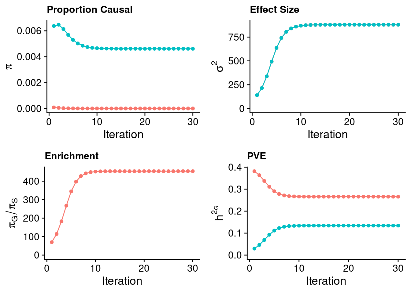
| Version | Author | Date |
|---|---|---|
| ce02b6f | wesleycrouse | 2023-08-18 |
#p_pi
#p_sigma2 + theme(legend.position = "none")
#p_enrich + theme(legend.position = "none")
#p_pve + theme(legend.position = "none")

####################

#estimated group prior
estimated_group_prior <- estimated_group_prior_all[,ncol(group_prior_rec)]
-sort(-estimated_group_prior)
gene SNP
0.0046166236 0.0000101777 #estimated group prior variance
estimated_group_prior_var <- estimated_group_prior_var_all[,ncol(group_prior_var_rec)]
-sort(-estimated_group_prior_var) SNP gene
879.4854 879.4854 #estimated enrichment
estimated_enrichment <- estimated_enrichment_all[,ncol(group_prior_var_rec)]
-sort(-estimated_enrichment) gene
453.602 #report sample size
print(sample_size)[1] 292933#report group size
print(group_size) SNP gene
8696600 9687 #estimated group PVE
estimated_group_pve <- estimated_group_pve_all[,ncol(group_prior_rec)]
-sort(-estimated_group_pve) SNP gene
0.2657415 0.1342685 #total PVE
sum(estimated_group_pve)[1] 0.4000099#attributable PVE
-sort(-estimated_group_pve/sum(estimated_group_pve)) SNP gene
0.6643371 0.3356629 Top genes by PIP
#genes with PIP>0.8 or 20 highest PIPs
head(ctwas_gene_res[order(-ctwas_gene_res$susie_pip),report_cols], max(sum(ctwas_gene_res$susie_pip>0.8), 20))
genename group region_tag susie_pip mu2 PVE z
9593 RP11-219B17.3 gene 15_27 0.9996749 56.39183 1.924450e-04 7.177095
9588 CCND2 gene 12_4 0.9956070 33.42255 1.135950e-04 5.337334
9586 RP11-452H21.4 gene 11_43 0.9950202 40.16688 1.364368e-04 5.936835
9594 CD276 gene 15_35 0.9946968 42.44094 1.441144e-04 6.126579
9518 HLA-G gene 6_24 0.9920415 50.24792 1.701687e-04 -6.693567
9559 DGAT2 gene 11_42 0.9827615 61.28181 2.055944e-04 -7.506981
9474 PRMT6 gene 1_66 0.9810956 31.41784 1.052251e-04 5.144273
9538 SMIM19 gene 8_37 0.9551178 36.01701 1.174347e-04 -5.575767
9479 INHBB gene 2_70 0.9419842 28.35770 9.118982e-05 4.805955
9541 CWF19L1 gene 10_64 0.9270493 32.21257 1.019436e-04 -6.866059
9524 IRAK1BP1 gene 6_54 0.9259852 28.72823 9.081230e-05 4.854598
9506 CSNK1G3 gene 5_75 0.9063806 27.97019 8.654416e-05 4.736926
9662 CYP2A6 gene 19_28 0.8983313 27.69709 8.493806e-05 -4.727496
9628 IL27 gene 16_23 0.8835765 28.20740 8.508223e-05 -4.759289
9481 ACVR1C gene 2_94 0.8667984 27.76038 8.214387e-05 4.615567
9504 GYPA gene 4_94 0.8633798 28.75209 8.474283e-05 4.825807
9482 CARF gene 2_120 0.8269404 27.54229 7.775099e-05 -4.635682
9466 PABPC4 gene 1_24 0.8168856 28.07394 7.828819e-05 4.515250
9632 MPO gene 17_34 0.7987496 28.24092 7.700542e-05 4.622761
7856 H3F3B gene 17_42 0.7827905 29.84913 7.976438e-05 5.277586Top variants by PIP
#genes with PIP>0.8 or 20 highest PIPs
head(ctwas_snp_res[order(-ctwas_snp_res$susie_pip),c("id","region_tag","susie_pip","mu2","z")], max(sum(ctwas_snp_res$susie_pip>0.8), 20))
id region_tag susie_pip mu2 z
327130 rs115740542 6_20 1.0000000 197.27989 -12.661774
603361 rs11045819 12_16 1.0000000 5723.32706 14.343399
887528 rs10179091 2_137 1.0000000 643983.75819 -204.743873
887555 rs1976391 2_137 1.0000000 637483.56470 -268.400608
887523 rs17863798 2_137 1.0000000 133739.59450 11.159348
533707 rs4745982 10_46 1.0000000 148.20657 -11.949194
327109 rs72834643 6_20 1.0000000 131.81787 -9.734124
370929 rs12208357 6_103 1.0000000 91.52293 6.654885
887552 rs11568318 2_137 0.9999999 137767.49822 65.812116
382715 rs542176135 7_17 0.9999841 177.75825 8.377159
802025 rs59616136 19_14 0.9999364 53.86043 -6.996600
603378 rs4363657 12_16 0.9999298 1629.55728 -43.784190
508995 rs115478735 9_70 0.9992295 69.25122 8.024314
382737 rs4721597 7_17 0.9986435 111.43940 -1.938467
328300 rs3130253 6_23 0.9982018 48.63152 6.634831
555002 rs76153913 11_2 0.9971519 53.73316 -6.696259
630634 rs653178 12_67 0.9961104 176.65578 13.120326
133585 rs4973550 2_136 0.9892815 45.26084 -6.179461
36468 rs2779116 1_78 0.9868122 72.86155 8.246902
603076 rs7962574 12_15 0.9823904 58.91351 8.397250
810167 rs814573 19_31 0.9797318 42.89949 6.681842
747931 rs2608604 16_53 0.9791943 45.64619 6.332841
802810 rs3794991 19_15 0.9560957 140.18711 -11.638289
810103 rs1551891 19_31 0.9499555 59.05794 -7.880338
133596 rs6731991 2_136 0.9413696 40.62472 5.751019
603116 rs10770693 12_15 0.9361150 67.01946 -8.859827
494914 rs9410381 9_45 0.9223063 79.09496 -8.615110
326948 rs75080831 6_19 0.8615419 68.27605 -7.955819
327679 rs156737 6_21 0.8482026 45.82333 6.370934
853141 rs6000553 22_14 0.8455982 46.81218 -6.466402
558024 rs4910498 11_8 0.8320924 50.12869 -6.708512
603262 rs12366506 12_16 0.8044615 4937.62648 -23.437259Case 35 - Bilirubin with Liver - Inv-Gamma prior on variance of SNPs and genes; a=2, b=10
Load ctwas results
results_dir <- paste0("/project2/mstephens/wcrouse/ctwas_multigroup_testing/ukb-d-30780_irnt/multigroup_case35")

weight <- "/project2/compbio/predictdb/mashr_models/mashr_Liver.db"

#load information for all genes

gene_info <- data.frame(gene=as.character(), genename=as.character(), gene_type=as.character(), weight=as.character())

for (i in 1:length(weight)){
  sqlite <- RSQLite::dbDriver("SQLite")
  db = RSQLite::dbConnect(sqlite, weight[i])
  query <- function(...) RSQLite::dbGetQuery(db, ...)
  gene_info_current <- query("select gene, genename, gene_type from extra")
  RSQLite::dbDisconnect(db)

  gene_info_current$weight <- weight[i]

  gene_info <- rbind(gene_info, gene_info_current)
}

gene_info$group <- sapply(1:nrow(gene_info), function(x){paste0(unlist(strsplit(tools::file_path_sans_ext(rev(unlist(strsplit(gene_info$weight[x], "/")))[1]), "_"))[-1], collapse="_")})

gene_info$gene_id <- paste(gene_info$gene, gene_info$group, sep="|")

# #load ctwas results
# ctwas_res <- data.table::fread(paste0(results_dir, "/", analysis_id, "_ctwas.susieIrss.txt"))
#
# #make unique identifier for regions
# ctwas_res$region_tag <- paste(ctwas_res$region_tag1, ctwas_res$region_tag2, sep="_")

#load z scores for SNPs and collect sample size
load(paste0(results_dir, "/", analysis_id, "_expr_z_snp.Rd"))

sample_size <- z_snp$ss
sample_size <- as.numeric(names(which.max(table(sample_size))))

# #compute PVE for each gene/SNP
# ctwas_res$PVE = ctwas_res$susie_pip*ctwas_res$mu2/sample_size
#
# #separate gene and SNP results
# ctwas_gene_res <- ctwas_res[ctwas_res$type != "SNP", ]
# ctwas_gene_res <- data.frame(ctwas_gene_res)
# ctwas_snp_res <- ctwas_res[ctwas_res$type == "SNP", ]
# ctwas_snp_res <- data.frame(ctwas_snp_res)
#
# #add gene information to results
# ctwas_gene_res$gene_id <- sapply(ctwas_gene_res$id, function(x){unlist(strsplit(x, split="[|]"))[1]})
# ctwas_gene_res$group <- ctwas_gene_res$type
# ctwas_gene_res$alt_name <- paste0(ctwas_gene_res$gene_id, "|", ctwas_gene_res$group)
#
# ctwas_gene_res$genename <- NA
# ctwas_gene_res$gene_type <- NA
#
# group_list <- unique(ctwas_gene_res$group)
#
# for (j in 1:length(group_list)){
#   print(j)
#   group <- group_list[j]
#
#   res_group_indx <- which(ctwas_gene_res$group==group)
#   gene_info_group <- gene_info[gene_info$group==group,,drop=F]
#
#   ctwas_gene_res[res_group_indx,c("genename", "gene_type")] <- gene_info_group[sapply(ctwas_gene_res$alt_name[res_group_indx], match, gene_info_group$gene_id), c("genename", "gene_type")]
# }

#add z scores to results
load(paste0(results_dir, "/", analysis_id, "_expr_z_gene.Rd"))
#ctwas_gene_res$z <- z_gene[ctwas_gene_res$id,]$z

#z_snp <- z_snp[z_snp$id %in% ctwas_snp_res$id,]
#ctwas_snp_res$z <- z_snp$z[match(ctwas_snp_res$id, z_snp$id)]

# #merge gene and snp results with added information
# ctwas_snp_res$gene_id=NA
# ctwas_snp_res$group="SNP"
# ctwas_snp_res$alt_name=NA
# ctwas_snp_res$genename=NA
# ctwas_snp_res$gene_type=NA
#
# ctwas_res <- rbind(ctwas_gene_res,
#                    ctwas_snp_res[,colnames(ctwas_gene_res)])

#get number of SNPs from s1 results; adjust for thin argument
ctwas_res_s1 <- data.table::fread(paste0(results_dir, "/", analysis_id, "_ctwas.s1.susieIrss.txt"))
n_snps <- sum(ctwas_res_s1$type=="SNP")/thin
rm(ctwas_res_s1)

# #store columns to report
# report_cols <- colnames(ctwas_gene_res)[!(colnames(ctwas_gene_res) %in% c("type", "region_tag1", "region_tag2", "cs_index", "gene_type", "z_flag", "id", "chrom", "pos", "alt_name", "gene_id"))]
# first_cols <- c("genename", "group", "region_tag")
# report_cols <- c(first_cols, report_cols[!(report_cols %in% first_cols)])
Check convergence of parameters
library(ggplot2)
library(cowplot)

load(paste0(results_dir, "/", analysis_id, "_ctwas.s2.susieIrssres.Rd"))

#estimated group prior (all iterations)
estimated_group_prior_all <- group_prior_rec
estimated_group_prior_all["SNP",] <- estimated_group_prior_all["SNP",]*thin #adjust parameter to account for thin argument

#estimated group prior variance (all iterations)
estimated_group_prior_var_all <- group_prior_var_rec

#set group size
group_size <- structure(c(n_snps, nrow(z_gene)), names=c("SNP","gene"))

#estimated group PVE (all iterations)
estimated_group_pve_all <- estimated_group_prior_var_all*estimated_group_prior_all*group_size/sample_size #check PVE calculation

#estimated enrichment of genes (all iterations)
estimated_enrichment_all <- t(sapply(rownames(estimated_group_prior_all)[rownames(estimated_group_prior_all)!="SNP"], function(x){estimated_group_prior_all[rownames(estimated_group_prior_all)==x,]/estimated_group_prior_all[rownames(estimated_group_prior_all)=="SNP"]}))

title_size <- 12

df <- data.frame(niter = rep(1:ncol(estimated_group_prior_all), nrow(estimated_group_prior_all)),
                 value = unlist(lapply(1:nrow(estimated_group_prior_all), function(x){estimated_group_prior_all[x,]})),
                 group = rep(rownames(estimated_group_prior_all), each=ncol(estimated_group_prior_all)))

groupnames_for_plots <- sapply(as.character(unique(df$group)), function(x){paste(sapply(unlist(strsplit(x, "_")), substr, start=1, stop=3), collapse="_")})

df$group <- groupnames_for_plots[df$group]
df$group <- as.factor(df$group)

p_pi <- ggplot(df, aes(x=niter, y=value, group=group)) +
  geom_line(aes(color=group)) +
  geom_point(aes(color=group)) +
  xlab("Iteration") + ylab(bquote(pi)) +
  ggtitle("Proportion Causal") +
  theme_cowplot()

p_pi <- p_pi + theme(plot.title=element_text(size=title_size)) +
  expand_limits(y=0) +
  guides(color = guide_legend(title = "Group")) + theme (legend.title = element_text(size=12, face="bold"))

df <- data.frame(niter = rep(1:ncol(estimated_group_prior_var_all), nrow(estimated_group_prior_var_all)),
                 value = unlist(lapply(1:nrow(estimated_group_prior_var_all), function(x){estimated_group_prior_var_all[x,]})),
                 group = rep(rownames(estimated_group_prior_var_all), each=ncol(estimated_group_prior_var_all)))

groupnames_for_plots <- sapply(as.character(unique(df$group)), function(x){paste(sapply(unlist(strsplit(x, "_")), substr, start=1, stop=3), collapse="_")})

df$group <- groupnames_for_plots[df$group]
df$group <- as.factor(df$group)

p_sigma2 <- ggplot(df, aes(x=niter, y=value, group=group)) +
  geom_line(aes(color=group)) +
  geom_point(aes(color=group)) +
  xlab("Iteration") + ylab(bquote(sigma^2)) +
  ggtitle("Effect Size") +
  theme_cowplot()

p_sigma2 <- p_sigma2 + theme(plot.title=element_text(size=title_size)) +
  expand_limits(y=0) +
  guides(color = guide_legend(title = "Group")) + theme (legend.title = element_text(size=12, face="bold"))

df <- data.frame(niter = rep(1:ncol(estimated_group_pve_all), nrow(estimated_group_pve_all)),
                 value = unlist(lapply(1:nrow(estimated_group_pve_all), function(x){estimated_group_pve_all[x,]})),
                 group = rep(rownames(estimated_group_pve_all), each=ncol(estimated_group_pve_all)))

groupnames_for_plots <- sapply(as.character(unique(df$group)), function(x){paste(sapply(unlist(strsplit(x, "_")), substr, start=1, stop=3), collapse="_")})

df$group <- groupnames_for_plots[df$group]
df$group <- as.factor(df$group)

p_pve <- ggplot(df, aes(x=niter, y=value, group=group)) +
  geom_line(aes(color=group)) +
  geom_point(aes(color=group)) +
  xlab("Iteration") + ylab(bquote(h^2[G])) +
  ggtitle("PVE") +
  theme_cowplot()

p_pve <- p_pve + theme(plot.title=element_text(size=title_size)) +
  expand_limits(y=0) +
  guides(color = guide_legend(title = "Group")) + theme (legend.title = element_text(size=12, face="bold"))

df <- data.frame(niter = rep(1:ncol(estimated_enrichment_all), nrow(estimated_enrichment_all)),
                 value = unlist(lapply(1:nrow(estimated_enrichment_all), function(x){estimated_enrichment_all[x,]})),
                 group = rep(rownames(estimated_enrichment_all), each=ncol(estimated_enrichment_all)))

groupnames_for_plots <- sapply(as.character(unique(df$group)), function(x){paste(sapply(unlist(strsplit(x, "_")), substr, start=1, stop=3), collapse="_")})

df$group <- groupnames_for_plots[df$group]
df$group <- as.factor(df$group)

p_enrich <- ggplot(df, aes(x=niter, y=value, group=group)) +
  geom_line(aes(color=group)) +
  geom_point(aes(color=group)) +
  xlab("Iteration") + ylab(bquote(pi[G]/pi[S])) +
  ggtitle("Enrichment") +
  theme_cowplot()

p_enrich <- p_enrich + theme(plot.title=element_text(size=title_size)) +
  expand_limits(y=0) +
  guides(color = guide_legend(title = "Group")) + theme (legend.title = element_text(size=12, face="bold"))

plot_grid(p_pi + theme(legend.position = "none"),
          p_sigma2 + theme(legend.position = "none"),
          p_enrich + theme(legend.position = "none"),
          p_pve+ theme(legend.position = "none"))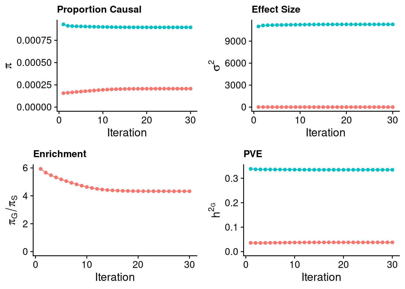
| Version | Author | Date |
|---|---|---|
| ce02b6f | wesleycrouse | 2023-08-18 |
#p_pi
#p_sigma2 + theme(legend.position = "none")
#p_enrich + theme(legend.position = "none")
#p_pve + theme(legend.position = "none")

####################

#estimated group prior
estimated_group_prior <- estimated_group_prior_all[,ncol(group_prior_rec)]
-sort(-estimated_group_prior)
gene SNP
0.0008957946 0.0002069582 #estimated group prior variance
estimated_group_prior_var <- estimated_group_prior_var_all[,ncol(group_prior_var_rec)]
-sort(-estimated_group_prior_var) gene SNP
11288.781541 6.160552 #estimated enrichment
estimated_enrichment <- estimated_enrichment_all[,ncol(group_prior_var_rec)]
-sort(-estimated_enrichment) gene
4.328384 #report sample size
print(sample_size)[1] 292933#report group size
print(group_size) SNP gene
8696600 9687 #estimated group PVE
estimated_group_pve <- estimated_group_pve_all[,ncol(group_prior_rec)]
-sort(-estimated_group_pve) gene SNP
0.33440788 0.03785153 #total PVE
sum(estimated_group_pve)[1] 0.3722594#attributable PVE
-sort(-estimated_group_pve/sum(estimated_group_pve)) gene SNP
0.8983195 0.1016805 Case 36 - Bilirubin with Liver - Inv-Gamma prior on variance of SNPs and genes; a=5, b=40
Load ctwas results
results_dir <- paste0("/project2/mstephens/wcrouse/ctwas_multigroup_testing/ukb-d-30780_irnt/multigroup_case36")

weight <- "/project2/compbio/predictdb/mashr_models/mashr_Liver.db"

#load information for all genes

gene_info <- data.frame(gene=as.character(), genename=as.character(), gene_type=as.character(), weight=as.character())

for (i in 1:length(weight)){
  sqlite <- RSQLite::dbDriver("SQLite")
  db = RSQLite::dbConnect(sqlite, weight[i])
  query <- function(...) RSQLite::dbGetQuery(db, ...)
  gene_info_current <- query("select gene, genename, gene_type from extra")
  RSQLite::dbDisconnect(db)

  gene_info_current$weight <- weight[i]

  gene_info <- rbind(gene_info, gene_info_current)
}

gene_info$group <- sapply(1:nrow(gene_info), function(x){paste0(unlist(strsplit(tools::file_path_sans_ext(rev(unlist(strsplit(gene_info$weight[x], "/")))[1]), "_"))[-1], collapse="_")})

gene_info$gene_id <- paste(gene_info$gene, gene_info$group, sep="|")

# #load ctwas results
# ctwas_res <- data.table::fread(paste0(results_dir, "/", analysis_id, "_ctwas.susieIrss.txt"))
#
# #make unique identifier for regions
# ctwas_res$region_tag <- paste(ctwas_res$region_tag1, ctwas_res$region_tag2, sep="_")

#load z scores for SNPs and collect sample size
load(paste0(results_dir, "/", analysis_id, "_expr_z_snp.Rd"))

sample_size <- z_snp$ss
sample_size <- as.numeric(names(which.max(table(sample_size))))

# #compute PVE for each gene/SNP
# ctwas_res$PVE = ctwas_res$susie_pip*ctwas_res$mu2/sample_size
#
# #separate gene and SNP results
# ctwas_gene_res <- ctwas_res[ctwas_res$type != "SNP", ]
# ctwas_gene_res <- data.frame(ctwas_gene_res)
# ctwas_snp_res <- ctwas_res[ctwas_res$type == "SNP", ]
# ctwas_snp_res <- data.frame(ctwas_snp_res)
#
# #add gene information to results
# ctwas_gene_res$gene_id <- sapply(ctwas_gene_res$id, function(x){unlist(strsplit(x, split="[|]"))[1]})
# ctwas_gene_res$group <- ctwas_gene_res$type
# ctwas_gene_res$alt_name <- paste0(ctwas_gene_res$gene_id, "|", ctwas_gene_res$group)
#
# ctwas_gene_res$genename <- NA
# ctwas_gene_res$gene_type <- NA
#
# group_list <- unique(ctwas_gene_res$group)
#
# for (j in 1:length(group_list)){
#   print(j)
#   group <- group_list[j]
#
#   res_group_indx <- which(ctwas_gene_res$group==group)
#   gene_info_group <- gene_info[gene_info$group==group,,drop=F]
#
#   ctwas_gene_res[res_group_indx,c("genename", "gene_type")] <- gene_info_group[sapply(ctwas_gene_res$alt_name[res_group_indx], match, gene_info_group$gene_id), c("genename", "gene_type")]
# }

#add z scores to results
load(paste0(results_dir, "/", analysis_id, "_expr_z_gene.Rd"))
#ctwas_gene_res$z <- z_gene[ctwas_gene_res$id,]$z

#z_snp <- z_snp[z_snp$id %in% ctwas_snp_res$id,]
#ctwas_snp_res$z <- z_snp$z[match(ctwas_snp_res$id, z_snp$id)]

# #merge gene and snp results with added information
# ctwas_snp_res$gene_id=NA
# ctwas_snp_res$group="SNP"
# ctwas_snp_res$alt_name=NA
# ctwas_snp_res$genename=NA
# ctwas_snp_res$gene_type=NA
#
# ctwas_res <- rbind(ctwas_gene_res,
#                    ctwas_snp_res[,colnames(ctwas_gene_res)])

#get number of SNPs from s1 results; adjust for thin argument
ctwas_res_s1 <- data.table::fread(paste0(results_dir, "/", analysis_id, "_ctwas.s1.susieIrss.txt"))
n_snps <- sum(ctwas_res_s1$type=="SNP")/thin
rm(ctwas_res_s1)

# #store columns to report
# report_cols <- colnames(ctwas_gene_res)[!(colnames(ctwas_gene_res) %in% c("type", "region_tag1", "region_tag2", "cs_index", "gene_type", "z_flag", "id", "chrom", "pos", "alt_name", "gene_id"))]
# first_cols <- c("genename", "group", "region_tag")
# report_cols <- c(first_cols, report_cols[!(report_cols %in% first_cols)])
Check convergence of parameters
library(ggplot2)
library(cowplot)

load(paste0(results_dir, "/", analysis_id, "_ctwas.s2.susieIrssres.Rd"))

#estimated group prior (all iterations)
estimated_group_prior_all <- group_prior_rec
estimated_group_prior_all["SNP",] <- estimated_group_prior_all["SNP",]*thin #adjust parameter to account for thin argument

#estimated group prior variance (all iterations)
estimated_group_prior_var_all <- group_prior_var_rec

#set group size
group_size <- structure(c(n_snps, nrow(z_gene)), names=c("SNP","gene"))

#estimated group PVE (all iterations)
estimated_group_pve_all <- estimated_group_prior_var_all*estimated_group_prior_all*group_size/sample_size #check PVE calculation

#estimated enrichment of genes (all iterations)
estimated_enrichment_all <- t(sapply(rownames(estimated_group_prior_all)[rownames(estimated_group_prior_all)!="SNP"], function(x){estimated_group_prior_all[rownames(estimated_group_prior_all)==x,]/estimated_group_prior_all[rownames(estimated_group_prior_all)=="SNP"]}))

title_size <- 12

df <- data.frame(niter = rep(1:ncol(estimated_group_prior_all), nrow(estimated_group_prior_all)),
                 value = unlist(lapply(1:nrow(estimated_group_prior_all), function(x){estimated_group_prior_all[x,]})),
                 group = rep(rownames(estimated_group_prior_all), each=ncol(estimated_group_prior_all)))

groupnames_for_plots <- sapply(as.character(unique(df$group)), function(x){paste(sapply(unlist(strsplit(x, "_")), substr, start=1, stop=3), collapse="_")})

df$group <- groupnames_for_plots[df$group]
df$group <- as.factor(df$group)

p_pi <- ggplot(df, aes(x=niter, y=value, group=group)) +
  geom_line(aes(color=group)) +
  geom_point(aes(color=group)) +
  xlab("Iteration") + ylab(bquote(pi)) +
  ggtitle("Proportion Causal") +
  theme_cowplot()

p_pi <- p_pi + theme(plot.title=element_text(size=title_size)) +
  expand_limits(y=0) +
  guides(color = guide_legend(title = "Group")) + theme (legend.title = element_text(size=12, face="bold"))

df <- data.frame(niter = rep(1:ncol(estimated_group_prior_var_all), nrow(estimated_group_prior_var_all)),
                 value = unlist(lapply(1:nrow(estimated_group_prior_var_all), function(x){estimated_group_prior_var_all[x,]})),
                 group = rep(rownames(estimated_group_prior_var_all), each=ncol(estimated_group_prior_var_all)))

groupnames_for_plots <- sapply(as.character(unique(df$group)), function(x){paste(sapply(unlist(strsplit(x, "_")), substr, start=1, stop=3), collapse="_")})

df$group <- groupnames_for_plots[df$group]
df$group <- as.factor(df$group)

p_sigma2 <- ggplot(df, aes(x=niter, y=value, group=group)) +
  geom_line(aes(color=group)) +
  geom_point(aes(color=group)) +
  xlab("Iteration") + ylab(bquote(sigma^2)) +
  ggtitle("Effect Size") +
  theme_cowplot()

p_sigma2 <- p_sigma2 + theme(plot.title=element_text(size=title_size)) +
  expand_limits(y=0) +
  guides(color = guide_legend(title = "Group")) + theme (legend.title = element_text(size=12, face="bold"))

df <- data.frame(niter = rep(1:ncol(estimated_group_pve_all), nrow(estimated_group_pve_all)),
                 value = unlist(lapply(1:nrow(estimated_group_pve_all), function(x){estimated_group_pve_all[x,]})),
                 group = rep(rownames(estimated_group_pve_all), each=ncol(estimated_group_pve_all)))

groupnames_for_plots <- sapply(as.character(unique(df$group)), function(x){paste(sapply(unlist(strsplit(x, "_")), substr, start=1, stop=3), collapse="_")})

df$group <- groupnames_for_plots[df$group]
df$group <- as.factor(df$group)

p_pve <- ggplot(df, aes(x=niter, y=value, group=group)) +
  geom_line(aes(color=group)) +
  geom_point(aes(color=group)) +
  xlab("Iteration") + ylab(bquote(h^2[G])) +
  ggtitle("PVE") +
  theme_cowplot()

p_pve <- p_pve + theme(plot.title=element_text(size=title_size)) +
  expand_limits(y=0) +
  guides(color = guide_legend(title = "Group")) + theme (legend.title = element_text(size=12, face="bold"))

df <- data.frame(niter = rep(1:ncol(estimated_enrichment_all), nrow(estimated_enrichment_all)),
                 value = unlist(lapply(1:nrow(estimated_enrichment_all), function(x){estimated_enrichment_all[x,]})),
                 group = rep(rownames(estimated_enrichment_all), each=ncol(estimated_enrichment_all)))

groupnames_for_plots <- sapply(as.character(unique(df$group)), function(x){paste(sapply(unlist(strsplit(x, "_")), substr, start=1, stop=3), collapse="_")})

df$group <- groupnames_for_plots[df$group]
df$group <- as.factor(df$group)

p_enrich <- ggplot(df, aes(x=niter, y=value, group=group)) +
  geom_line(aes(color=group)) +
  geom_point(aes(color=group)) +
  xlab("Iteration") + ylab(bquote(pi[G]/pi[S])) +
  ggtitle("Enrichment") +
  theme_cowplot()

p_enrich <- p_enrich + theme(plot.title=element_text(size=title_size)) +
  expand_limits(y=0) +
  guides(color = guide_legend(title = "Group")) + theme (legend.title = element_text(size=12, face="bold"))

plot_grid(p_pi + theme(legend.position = "none"),
          p_sigma2 + theme(legend.position = "none"),
          p_enrich + theme(legend.position = "none"),
          p_pve+ theme(legend.position = "none"))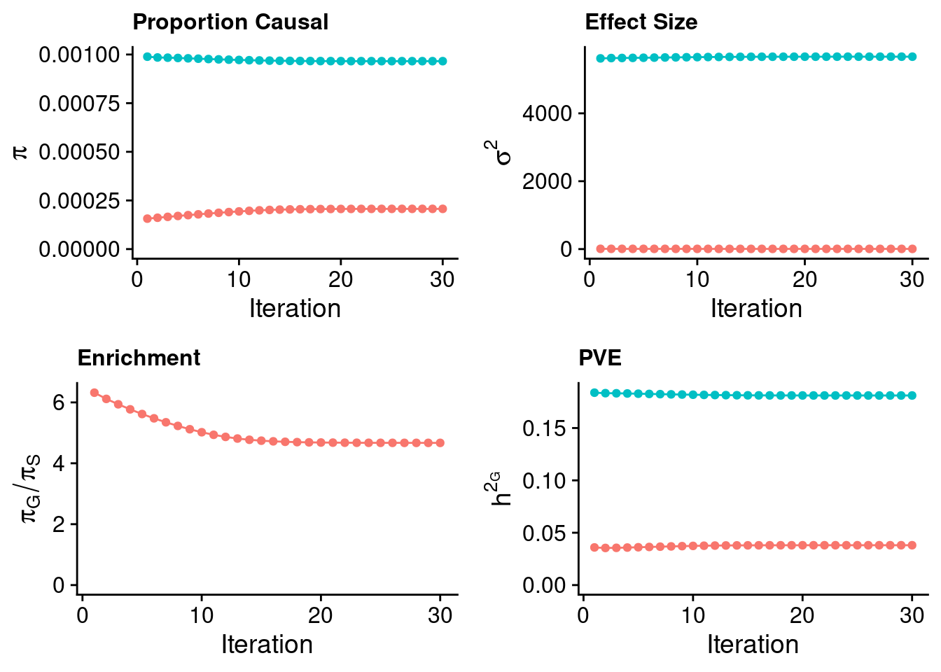
| Version | Author | Date |
|---|---|---|
| ce02b6f | wesleycrouse | 2023-08-18 |
#p_pi
#p_sigma2 + theme(legend.position = "none")
#p_enrich + theme(legend.position = "none")
#p_pve + theme(legend.position = "none")

####################

#estimated group prior
estimated_group_prior <- estimated_group_prior_all[,ncol(group_prior_rec)]
-sort(-estimated_group_prior)
gene SNP
0.0009658282 0.0002067951 #estimated group prior variance
estimated_group_prior_var <- estimated_group_prior_var_all[,ncol(group_prior_var_rec)]
-sort(-estimated_group_prior_var) gene SNP
5669.185717 6.200549 #estimated enrichment
estimated_enrichment <- estimated_enrichment_all[,ncol(group_prior_var_rec)]
-sort(-estimated_enrichment) gene
4.67046 #report sample size
print(sample_size)[1] 292933#report group size
print(group_size) SNP gene
8696600 9687 #estimated group PVE
estimated_group_pve <- estimated_group_pve_all[,ncol(group_prior_rec)]
-sort(-estimated_group_pve) gene SNP
0.18106793 0.03806725 #total PVE
sum(estimated_group_pve)[1] 0.2191352#attributable PVE
-sort(-estimated_group_pve/sum(estimated_group_pve)) gene SNP
0.8262842 0.1737158 Case 37 - Bilirubin with Liver - Inv-Gamma prior on variance of SNPs and genes; a=41, b=400
Load ctwas results
results_dir <- paste0("/project2/mstephens/wcrouse/ctwas_multigroup_testing/ukb-d-30780_irnt/multigroup_case37")

weight <- "/project2/compbio/predictdb/mashr_models/mashr_Liver.db"

#load information for all genes

gene_info <- data.frame(gene=as.character(), genename=as.character(), gene_type=as.character(), weight=as.character())

for (i in 1:length(weight)){
  sqlite <- RSQLite::dbDriver("SQLite")
  db = RSQLite::dbConnect(sqlite, weight[i])
  query <- function(...) RSQLite::dbGetQuery(db, ...)
  gene_info_current <- query("select gene, genename, gene_type from extra")
  RSQLite::dbDisconnect(db)

  gene_info_current$weight <- weight[i]

  gene_info <- rbind(gene_info, gene_info_current)
}

gene_info$group <- sapply(1:nrow(gene_info), function(x){paste0(unlist(strsplit(tools::file_path_sans_ext(rev(unlist(strsplit(gene_info$weight[x], "/")))[1]), "_"))[-1], collapse="_")})

gene_info$gene_id <- paste(gene_info$gene, gene_info$group, sep="|")

# #load ctwas results
# ctwas_res <- data.table::fread(paste0(results_dir, "/", analysis_id, "_ctwas.susieIrss.txt"))
#
# #make unique identifier for regions
# ctwas_res$region_tag <- paste(ctwas_res$region_tag1, ctwas_res$region_tag2, sep="_")

#load z scores for SNPs and collect sample size
load(paste0(results_dir, "/", analysis_id, "_expr_z_snp.Rd"))

sample_size <- z_snp$ss
sample_size <- as.numeric(names(which.max(table(sample_size))))

# #compute PVE for each gene/SNP
# ctwas_res$PVE = ctwas_res$susie_pip*ctwas_res$mu2/sample_size
#
# #separate gene and SNP results
# ctwas_gene_res <- ctwas_res[ctwas_res$type != "SNP", ]
# ctwas_gene_res <- data.frame(ctwas_gene_res)
# ctwas_snp_res <- ctwas_res[ctwas_res$type == "SNP", ]
# ctwas_snp_res <- data.frame(ctwas_snp_res)
#
# #add gene information to results
# ctwas_gene_res$gene_id <- sapply(ctwas_gene_res$id, function(x){unlist(strsplit(x, split="[|]"))[1]})
# ctwas_gene_res$group <- ctwas_gene_res$type
# ctwas_gene_res$alt_name <- paste0(ctwas_gene_res$gene_id, "|", ctwas_gene_res$group)
#
# ctwas_gene_res$genename <- NA
# ctwas_gene_res$gene_type <- NA
#
# group_list <- unique(ctwas_gene_res$group)
#
# for (j in 1:length(group_list)){
#   print(j)
#   group <- group_list[j]
#
#   res_group_indx <- which(ctwas_gene_res$group==group)
#   gene_info_group <- gene_info[gene_info$group==group,,drop=F]
#
#   ctwas_gene_res[res_group_indx,c("genename", "gene_type")] <- gene_info_group[sapply(ctwas_gene_res$alt_name[res_group_indx], match, gene_info_group$gene_id), c("genename", "gene_type")]
# }

#add z scores to results
load(paste0(results_dir, "/", analysis_id, "_expr_z_gene.Rd"))
#ctwas_gene_res$z <- z_gene[ctwas_gene_res$id,]$z

#z_snp <- z_snp[z_snp$id %in% ctwas_snp_res$id,]
#ctwas_snp_res$z <- z_snp$z[match(ctwas_snp_res$id, z_snp$id)]

# #merge gene and snp results with added information
# ctwas_snp_res$gene_id=NA
# ctwas_snp_res$group="SNP"
# ctwas_snp_res$alt_name=NA
# ctwas_snp_res$genename=NA
# ctwas_snp_res$gene_type=NA
#
# ctwas_res <- rbind(ctwas_gene_res,
#                    ctwas_snp_res[,colnames(ctwas_gene_res)])

#get number of SNPs from s1 results; adjust for thin argument
ctwas_res_s1 <- data.table::fread(paste0(results_dir, "/", analysis_id, "_ctwas.s1.susieIrss.txt"))
n_snps <- sum(ctwas_res_s1$type=="SNP")/thin
rm(ctwas_res_s1)

# #store columns to report
# report_cols <- colnames(ctwas_gene_res)[!(colnames(ctwas_gene_res) %in% c("type", "region_tag1", "region_tag2", "cs_index", "gene_type", "z_flag", "id", "chrom", "pos", "alt_name", "gene_id"))]
# first_cols <- c("genename", "group", "region_tag")
# report_cols <- c(first_cols, report_cols[!(report_cols %in% first_cols)])
Check convergence of parameters
library(ggplot2)
library(cowplot)

load(paste0(results_dir, "/", analysis_id, "_ctwas.s2.susieIrssres.Rd"))

#estimated group prior (all iterations)
estimated_group_prior_all <- group_prior_rec
estimated_group_prior_all["SNP",] <- estimated_group_prior_all["SNP",]*thin #adjust parameter to account for thin argument

#estimated group prior variance (all iterations)
estimated_group_prior_var_all <- group_prior_var_rec

#set group size
group_size <- structure(c(n_snps, nrow(z_gene)), names=c("SNP","gene"))

#estimated group PVE (all iterations)
estimated_group_pve_all <- estimated_group_prior_var_all*estimated_group_prior_all*group_size/sample_size #check PVE calculation

#estimated enrichment of genes (all iterations)
estimated_enrichment_all <- t(sapply(rownames(estimated_group_prior_all)[rownames(estimated_group_prior_all)!="SNP"], function(x){estimated_group_prior_all[rownames(estimated_group_prior_all)==x,]/estimated_group_prior_all[rownames(estimated_group_prior_all)=="SNP"]}))

title_size <- 12

df <- data.frame(niter = rep(1:ncol(estimated_group_prior_all), nrow(estimated_group_prior_all)),
                 value = unlist(lapply(1:nrow(estimated_group_prior_all), function(x){estimated_group_prior_all[x,]})),
                 group = rep(rownames(estimated_group_prior_all), each=ncol(estimated_group_prior_all)))

groupnames_for_plots <- sapply(as.character(unique(df$group)), function(x){paste(sapply(unlist(strsplit(x, "_")), substr, start=1, stop=3), collapse="_")})

df$group <- groupnames_for_plots[df$group]
df$group <- as.factor(df$group)

p_pi <- ggplot(df, aes(x=niter, y=value, group=group)) +
  geom_line(aes(color=group)) +
  geom_point(aes(color=group)) +
  xlab("Iteration") + ylab(bquote(pi)) +
  ggtitle("Proportion Causal") +
  theme_cowplot()

p_pi <- p_pi + theme(plot.title=element_text(size=title_size)) +
  expand_limits(y=0) +
  guides(color = guide_legend(title = "Group")) + theme (legend.title = element_text(size=12, face="bold"))

df <- data.frame(niter = rep(1:ncol(estimated_group_prior_var_all), nrow(estimated_group_prior_var_all)),
                 value = unlist(lapply(1:nrow(estimated_group_prior_var_all), function(x){estimated_group_prior_var_all[x,]})),
                 group = rep(rownames(estimated_group_prior_var_all), each=ncol(estimated_group_prior_var_all)))

groupnames_for_plots <- sapply(as.character(unique(df$group)), function(x){paste(sapply(unlist(strsplit(x, "_")), substr, start=1, stop=3), collapse="_")})

df$group <- groupnames_for_plots[df$group]
df$group <- as.factor(df$group)

p_sigma2 <- ggplot(df, aes(x=niter, y=value, group=group)) +
  geom_line(aes(color=group)) +
  geom_point(aes(color=group)) +
  xlab("Iteration") + ylab(bquote(sigma^2)) +
  ggtitle("Effect Size") +
  theme_cowplot()

p_sigma2 <- p_sigma2 + theme(plot.title=element_text(size=title_size)) +
  expand_limits(y=0) +
  guides(color = guide_legend(title = "Group")) + theme (legend.title = element_text(size=12, face="bold"))

df <- data.frame(niter = rep(1:ncol(estimated_group_pve_all), nrow(estimated_group_pve_all)),
                 value = unlist(lapply(1:nrow(estimated_group_pve_all), function(x){estimated_group_pve_all[x,]})),
                 group = rep(rownames(estimated_group_pve_all), each=ncol(estimated_group_pve_all)))

groupnames_for_plots <- sapply(as.character(unique(df$group)), function(x){paste(sapply(unlist(strsplit(x, "_")), substr, start=1, stop=3), collapse="_")})

df$group <- groupnames_for_plots[df$group]
df$group <- as.factor(df$group)

p_pve <- ggplot(df, aes(x=niter, y=value, group=group)) +
  geom_line(aes(color=group)) +
  geom_point(aes(color=group)) +
  xlab("Iteration") + ylab(bquote(h^2[G])) +
  ggtitle("PVE") +
  theme_cowplot()

p_pve <- p_pve + theme(plot.title=element_text(size=title_size)) +
  expand_limits(y=0) +
  guides(color = guide_legend(title = "Group")) + theme (legend.title = element_text(size=12, face="bold"))

df <- data.frame(niter = rep(1:ncol(estimated_enrichment_all), nrow(estimated_enrichment_all)),
                 value = unlist(lapply(1:nrow(estimated_enrichment_all), function(x){estimated_enrichment_all[x,]})),
                 group = rep(rownames(estimated_enrichment_all), each=ncol(estimated_enrichment_all)))

groupnames_for_plots <- sapply(as.character(unique(df$group)), function(x){paste(sapply(unlist(strsplit(x, "_")), substr, start=1, stop=3), collapse="_")})

df$group <- groupnames_for_plots[df$group]
df$group <- as.factor(df$group)

p_enrich <- ggplot(df, aes(x=niter, y=value, group=group)) +
  geom_line(aes(color=group)) +
  geom_point(aes(color=group)) +
  xlab("Iteration") + ylab(bquote(pi[G]/pi[S])) +
  ggtitle("Enrichment") +
  theme_cowplot()

p_enrich <- p_enrich + theme(plot.title=element_text(size=title_size)) +
  expand_limits(y=0) +
  guides(color = guide_legend(title = "Group")) + theme (legend.title = element_text(size=12, face="bold"))

plot_grid(p_pi + theme(legend.position = "none"),
          p_sigma2 + theme(legend.position = "none"),
          p_enrich + theme(legend.position = "none"),
          p_pve+ theme(legend.position = "none"))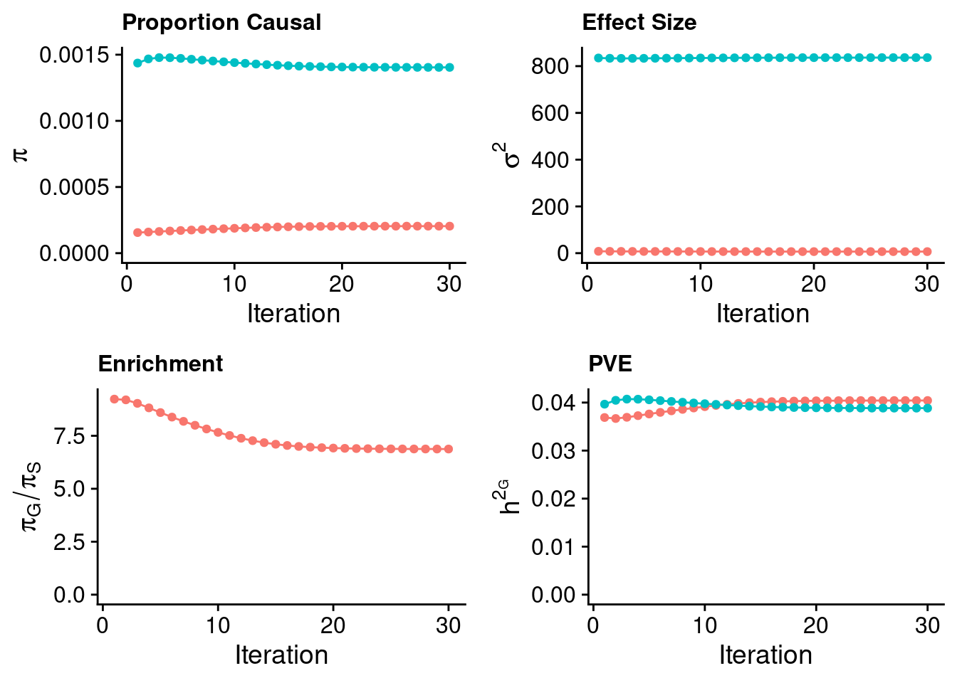
| Version | Author | Date |
|---|---|---|
| ce02b6f | wesleycrouse | 2023-08-18 |
#p_pi
#p_sigma2 + theme(legend.position = "none")
#p_enrich + theme(legend.position = "none")
#p_pve + theme(legend.position = "none")

####################

#estimated group prior
estimated_group_prior <- estimated_group_prior_all[,ncol(group_prior_rec)]
-sort(-estimated_group_prior)
gene SNP
0.0014040979 0.0002042366 #estimated group prior variance
estimated_group_prior_var <- estimated_group_prior_var_all[,ncol(group_prior_var_rec)]
-sort(-estimated_group_prior_var) gene SNP
836.537388 6.667974 #estimated enrichment
estimated_enrichment <- estimated_enrichment_all[,ncol(group_prior_var_rec)]
-sort(-estimated_enrichment) gene
6.874859 #report sample size
print(sample_size)[1] 292933#report group size
print(group_size) SNP gene
8696600 9687 #estimated group PVE
estimated_group_pve <- estimated_group_pve_all[,ncol(group_prior_rec)]
-sort(-estimated_group_pve) SNP gene
0.04043046 0.03884219 #total PVE
sum(estimated_group_pve)[1] 0.07927265#attributable PVE
-sort(-estimated_group_pve/sum(estimated_group_pve)) SNP gene
0.5100177 0.4899823 Case 39 - Bilirubin with Liver - Inv-Gamma prior on variance of SNPs and genes; a=401, b=4000
Load ctwas results
results_dir <- paste0("/project2/mstephens/wcrouse/ctwas_multigroup_testing/ukb-d-30780_irnt/multigroup_case39")

weight <- "/project2/compbio/predictdb/mashr_models/mashr_Liver.db"

#load information for all genes

gene_info <- data.frame(gene=as.character(), genename=as.character(), gene_type=as.character(), weight=as.character())

for (i in 1:length(weight)){
  sqlite <- RSQLite::dbDriver("SQLite")
  db = RSQLite::dbConnect(sqlite, weight[i])
  query <- function(...) RSQLite::dbGetQuery(db, ...)
  gene_info_current <- query("select gene, genename, gene_type from extra")
  RSQLite::dbDisconnect(db)

  gene_info_current$weight <- weight[i]

  gene_info <- rbind(gene_info, gene_info_current)
}

gene_info$group <- sapply(1:nrow(gene_info), function(x){paste0(unlist(strsplit(tools::file_path_sans_ext(rev(unlist(strsplit(gene_info$weight[x], "/")))[1]), "_"))[-1], collapse="_")})

gene_info$gene_id <- paste(gene_info$gene, gene_info$group, sep="|")

# #load ctwas results
# ctwas_res <- data.table::fread(paste0(results_dir, "/", analysis_id, "_ctwas.susieIrss.txt"))
#
# #make unique identifier for regions
# ctwas_res$region_tag <- paste(ctwas_res$region_tag1, ctwas_res$region_tag2, sep="_")

#load z scores for SNPs and collect sample size
load(paste0(results_dir, "/", analysis_id, "_expr_z_snp.Rd"))

sample_size <- z_snp$ss
sample_size <- as.numeric(names(which.max(table(sample_size))))

# #compute PVE for each gene/SNP
# ctwas_res$PVE = ctwas_res$susie_pip*ctwas_res$mu2/sample_size
#
# #separate gene and SNP results
# ctwas_gene_res <- ctwas_res[ctwas_res$type != "SNP", ]
# ctwas_gene_res <- data.frame(ctwas_gene_res)
# ctwas_snp_res <- ctwas_res[ctwas_res$type == "SNP", ]
# ctwas_snp_res <- data.frame(ctwas_snp_res)
#
# #add gene information to results
# ctwas_gene_res$gene_id <- sapply(ctwas_gene_res$id, function(x){unlist(strsplit(x, split="[|]"))[1]})
# ctwas_gene_res$group <- ctwas_gene_res$type
# ctwas_gene_res$alt_name <- paste0(ctwas_gene_res$gene_id, "|", ctwas_gene_res$group)
#
# ctwas_gene_res$genename <- NA
# ctwas_gene_res$gene_type <- NA
#
# group_list <- unique(ctwas_gene_res$group)
#
# for (j in 1:length(group_list)){
#   print(j)
#   group <- group_list[j]
#
#   res_group_indx <- which(ctwas_gene_res$group==group)
#   gene_info_group <- gene_info[gene_info$group==group,,drop=F]
#
#   ctwas_gene_res[res_group_indx,c("genename", "gene_type")] <- gene_info_group[sapply(ctwas_gene_res$alt_name[res_group_indx], match, gene_info_group$gene_id), c("genename", "gene_type")]
# }

#add z scores to results
load(paste0(results_dir, "/", analysis_id, "_expr_z_gene.Rd"))
#ctwas_gene_res$z <- z_gene[ctwas_gene_res$id,]$z

#z_snp <- z_snp[z_snp$id %in% ctwas_snp_res$id,]
#ctwas_snp_res$z <- z_snp$z[match(ctwas_snp_res$id, z_snp$id)]

# #merge gene and snp results with added information
# ctwas_snp_res$gene_id=NA
# ctwas_snp_res$group="SNP"
# ctwas_snp_res$alt_name=NA
# ctwas_snp_res$genename=NA
# ctwas_snp_res$gene_type=NA
#
# ctwas_res <- rbind(ctwas_gene_res,
#                    ctwas_snp_res[,colnames(ctwas_gene_res)])

#get number of SNPs from s1 results; adjust for thin argument
ctwas_res_s1 <- data.table::fread(paste0(results_dir, "/", analysis_id, "_ctwas.s1.susieIrss.txt"))
n_snps <- sum(ctwas_res_s1$type=="SNP")/thin
rm(ctwas_res_s1)

# #store columns to report
# report_cols <- colnames(ctwas_gene_res)[!(colnames(ctwas_gene_res) %in% c("type", "region_tag1", "region_tag2", "cs_index", "gene_type", "z_flag", "id", "chrom", "pos", "alt_name", "gene_id"))]
# first_cols <- c("genename", "group", "region_tag")
# report_cols <- c(first_cols, report_cols[!(report_cols %in% first_cols)])
Check convergence of parameters
library(ggplot2)
library(cowplot)

load(paste0(results_dir, "/", analysis_id, "_ctwas.s2.susieIrssres.Rd"))

#estimated group prior (all iterations)
estimated_group_prior_all <- group_prior_rec
estimated_group_prior_all["SNP",] <- estimated_group_prior_all["SNP",]*thin #adjust parameter to account for thin argument

#estimated group prior variance (all iterations)
estimated_group_prior_var_all <- group_prior_var_rec

#set group size
group_size <- structure(c(n_snps, nrow(z_gene)), names=c("SNP","gene"))

#estimated group PVE (all iterations)
estimated_group_pve_all <- estimated_group_prior_var_all*estimated_group_prior_all*group_size/sample_size #check PVE calculation

#estimated enrichment of genes (all iterations)
estimated_enrichment_all <- t(sapply(rownames(estimated_group_prior_all)[rownames(estimated_group_prior_all)!="SNP"], function(x){estimated_group_prior_all[rownames(estimated_group_prior_all)==x,]/estimated_group_prior_all[rownames(estimated_group_prior_all)=="SNP"]}))

title_size <- 12

df <- data.frame(niter = rep(1:ncol(estimated_group_prior_all), nrow(estimated_group_prior_all)),
                 value = unlist(lapply(1:nrow(estimated_group_prior_all), function(x){estimated_group_prior_all[x,]})),
                 group = rep(rownames(estimated_group_prior_all), each=ncol(estimated_group_prior_all)))

groupnames_for_plots <- sapply(as.character(unique(df$group)), function(x){paste(sapply(unlist(strsplit(x, "_")), substr, start=1, stop=3), collapse="_")})

df$group <- groupnames_for_plots[df$group]
df$group <- as.factor(df$group)

p_pi <- ggplot(df, aes(x=niter, y=value, group=group)) +
  geom_line(aes(color=group)) +
  geom_point(aes(color=group)) +
  xlab("Iteration") + ylab(bquote(pi)) +
  ggtitle("Proportion Causal") +
  theme_cowplot()

p_pi <- p_pi + theme(plot.title=element_text(size=title_size)) +
  expand_limits(y=0) +
  guides(color = guide_legend(title = "Group")) + theme (legend.title = element_text(size=12, face="bold"))

df <- data.frame(niter = rep(1:ncol(estimated_group_prior_var_all), nrow(estimated_group_prior_var_all)),
                 value = unlist(lapply(1:nrow(estimated_group_prior_var_all), function(x){estimated_group_prior_var_all[x,]})),
                 group = rep(rownames(estimated_group_prior_var_all), each=ncol(estimated_group_prior_var_all)))

groupnames_for_plots <- sapply(as.character(unique(df$group)), function(x){paste(sapply(unlist(strsplit(x, "_")), substr, start=1, stop=3), collapse="_")})

df$group <- groupnames_for_plots[df$group]
df$group <- as.factor(df$group)

p_sigma2 <- ggplot(df, aes(x=niter, y=value, group=group)) +
  geom_line(aes(color=group)) +
  geom_point(aes(color=group)) +
  xlab("Iteration") + ylab(bquote(sigma^2)) +
  ggtitle("Effect Size") +
  theme_cowplot()

p_sigma2 <- p_sigma2 + theme(plot.title=element_text(size=title_size)) +
  expand_limits(y=0) +
  guides(color = guide_legend(title = "Group")) + theme (legend.title = element_text(size=12, face="bold"))

df <- data.frame(niter = rep(1:ncol(estimated_group_pve_all), nrow(estimated_group_pve_all)),
                 value = unlist(lapply(1:nrow(estimated_group_pve_all), function(x){estimated_group_pve_all[x,]})),
                 group = rep(rownames(estimated_group_pve_all), each=ncol(estimated_group_pve_all)))

groupnames_for_plots <- sapply(as.character(unique(df$group)), function(x){paste(sapply(unlist(strsplit(x, "_")), substr, start=1, stop=3), collapse="_")})

df$group <- groupnames_for_plots[df$group]
df$group <- as.factor(df$group)

p_pve <- ggplot(df, aes(x=niter, y=value, group=group)) +
  geom_line(aes(color=group)) +
  geom_point(aes(color=group)) +
  xlab("Iteration") + ylab(bquote(h^2[G])) +
  ggtitle("PVE") +
  theme_cowplot()

p_pve <- p_pve + theme(plot.title=element_text(size=title_size)) +
  expand_limits(y=0) +
  guides(color = guide_legend(title = "Group")) + theme (legend.title = element_text(size=12, face="bold"))

df <- data.frame(niter = rep(1:ncol(estimated_enrichment_all), nrow(estimated_enrichment_all)),
                 value = unlist(lapply(1:nrow(estimated_enrichment_all), function(x){estimated_enrichment_all[x,]})),
                 group = rep(rownames(estimated_enrichment_all), each=ncol(estimated_enrichment_all)))

groupnames_for_plots <- sapply(as.character(unique(df$group)), function(x){paste(sapply(unlist(strsplit(x, "_")), substr, start=1, stop=3), collapse="_")})

df$group <- groupnames_for_plots[df$group]
df$group <- as.factor(df$group)

p_enrich <- ggplot(df, aes(x=niter, y=value, group=group)) +
  geom_line(aes(color=group)) +
  geom_point(aes(color=group)) +
  xlab("Iteration") + ylab(bquote(pi[G]/pi[S])) +
  ggtitle("Enrichment") +
  theme_cowplot()

p_enrich <- p_enrich + theme(plot.title=element_text(size=title_size)) +
  expand_limits(y=0) +
  guides(color = guide_legend(title = "Group")) + theme (legend.title = element_text(size=12, face="bold"))

plot_grid(p_pi + theme(legend.position = "none"),
          p_sigma2 + theme(legend.position = "none"),
          p_enrich + theme(legend.position = "none"),
          p_pve+ theme(legend.position = "none"))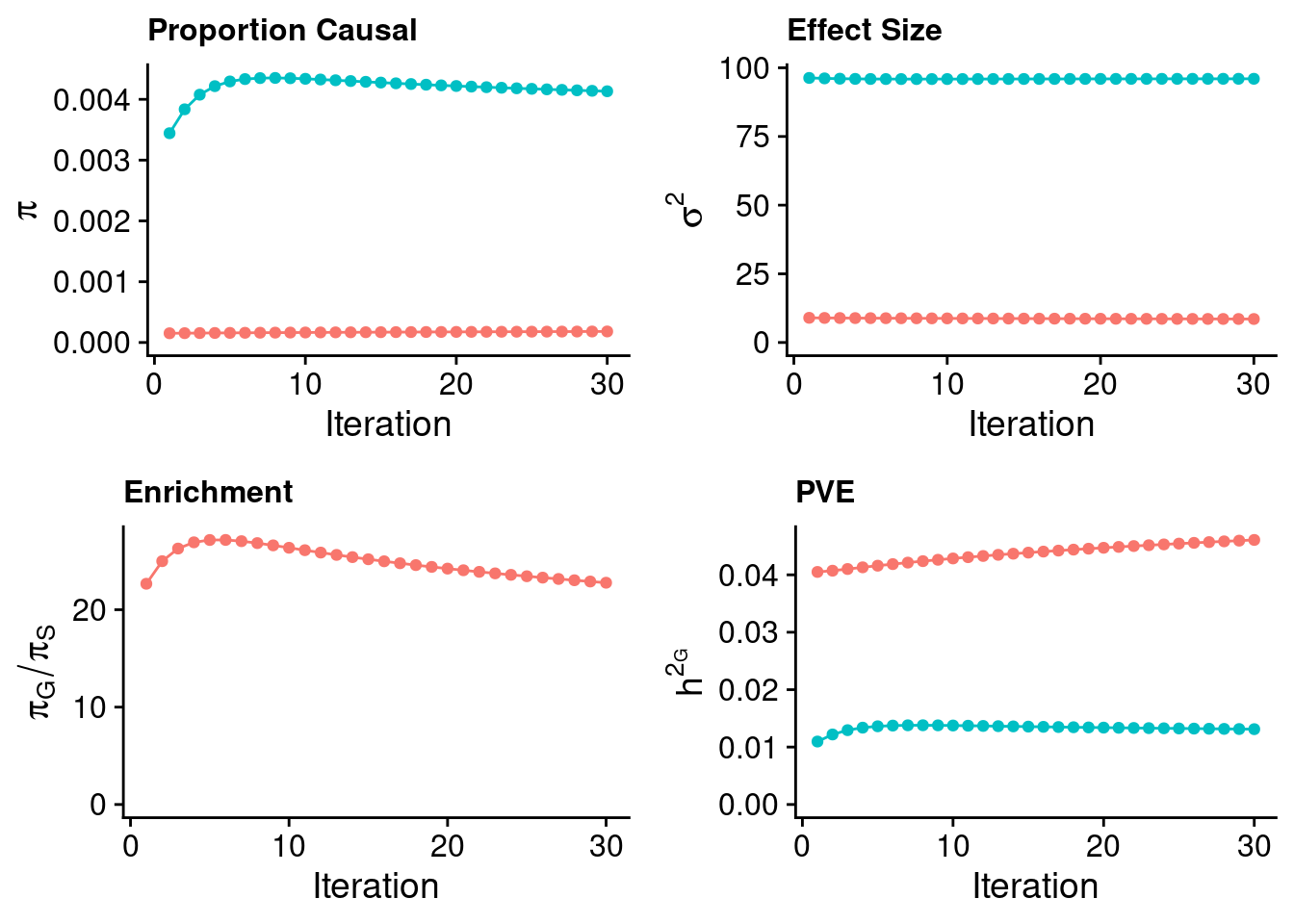
#p_pi
#p_sigma2 + theme(legend.position = "none")
#p_enrich + theme(legend.position = "none")
#p_pve + theme(legend.position = "none")

####################

#estimated group prior
estimated_group_prior <- estimated_group_prior_all[,ncol(group_prior_rec)]
-sort(-estimated_group_prior)
gene SNP
0.0041325068 0.0001814764 #estimated group prior variance
estimated_group_prior_var <- estimated_group_prior_var_all[,ncol(group_prior_var_rec)]
-sort(-estimated_group_prior_var) gene SNP
95.997710 8.552013 #estimated enrichment
estimated_enrichment <- estimated_enrichment_all[,ncol(group_prior_var_rec)]
-sort(-estimated_enrichment) gene
22.7716 #report sample size
print(sample_size)[1] 292933#report group size
print(group_size) SNP gene
8696600 9687 #estimated group PVE
estimated_group_pve <- estimated_group_pve_all[,ncol(group_prior_rec)]
-sort(-estimated_group_pve) SNP gene
0.04607546 0.01311884 #total PVE
sum(estimated_group_pve)[1] 0.0591943#attributable PVE
-sort(-estimated_group_pve/sum(estimated_group_pve)) SNP gene
0.7783766 0.2216234 Case 40 - Bilirubin with Liver - Inv-Gamma prior on variance of SNPs and genes; a=4001, b=40000
Load ctwas results
results_dir <- paste0("/project2/mstephens/wcrouse/ctwas_multigroup_testing/ukb-d-30780_irnt/multigroup_case40")

weight <- "/project2/compbio/predictdb/mashr_models/mashr_Liver.db"

#load information for all genes

gene_info <- data.frame(gene=as.character(), genename=as.character(), gene_type=as.character(), weight=as.character())

for (i in 1:length(weight)){
  sqlite <- RSQLite::dbDriver("SQLite")
  db = RSQLite::dbConnect(sqlite, weight[i])
  query <- function(...) RSQLite::dbGetQuery(db, ...)
  gene_info_current <- query("select gene, genename, gene_type from extra")
  RSQLite::dbDisconnect(db)

  gene_info_current$weight <- weight[i]

  gene_info <- rbind(gene_info, gene_info_current)
}

gene_info$group <- sapply(1:nrow(gene_info), function(x){paste0(unlist(strsplit(tools::file_path_sans_ext(rev(unlist(strsplit(gene_info$weight[x], "/")))[1]), "_"))[-1], collapse="_")})

gene_info$gene_id <- paste(gene_info$gene, gene_info$group, sep="|")

# #load ctwas results
# ctwas_res <- data.table::fread(paste0(results_dir, "/", analysis_id, "_ctwas.susieIrss.txt"))
#
# #make unique identifier for regions
# ctwas_res$region_tag <- paste(ctwas_res$region_tag1, ctwas_res$region_tag2, sep="_")

#load z scores for SNPs and collect sample size
load(paste0(results_dir, "/", analysis_id, "_expr_z_snp.Rd"))

sample_size <- z_snp$ss
sample_size <- as.numeric(names(which.max(table(sample_size))))

# #compute PVE for each gene/SNP
# ctwas_res$PVE = ctwas_res$susie_pip*ctwas_res$mu2/sample_size
#
# #separate gene and SNP results
# ctwas_gene_res <- ctwas_res[ctwas_res$type != "SNP", ]
# ctwas_gene_res <- data.frame(ctwas_gene_res)
# ctwas_snp_res <- ctwas_res[ctwas_res$type == "SNP", ]
# ctwas_snp_res <- data.frame(ctwas_snp_res)
#
# #add gene information to results
# ctwas_gene_res$gene_id <- sapply(ctwas_gene_res$id, function(x){unlist(strsplit(x, split="[|]"))[1]})
# ctwas_gene_res$group <- ctwas_gene_res$type
# ctwas_gene_res$alt_name <- paste0(ctwas_gene_res$gene_id, "|", ctwas_gene_res$group)
#
# ctwas_gene_res$genename <- NA
# ctwas_gene_res$gene_type <- NA
#
# group_list <- unique(ctwas_gene_res$group)
#
# for (j in 1:length(group_list)){
#   print(j)
#   group <- group_list[j]
#
#   res_group_indx <- which(ctwas_gene_res$group==group)
#   gene_info_group <- gene_info[gene_info$group==group,,drop=F]
#
#   ctwas_gene_res[res_group_indx,c("genename", "gene_type")] <- gene_info_group[sapply(ctwas_gene_res$alt_name[res_group_indx], match, gene_info_group$gene_id), c("genename", "gene_type")]
# }

#add z scores to results
load(paste0(results_dir, "/", analysis_id, "_expr_z_gene.Rd"))
#ctwas_gene_res$z <- z_gene[ctwas_gene_res$id,]$z

#z_snp <- z_snp[z_snp$id %in% ctwas_snp_res$id,]
#ctwas_snp_res$z <- z_snp$z[match(ctwas_snp_res$id, z_snp$id)]

# #merge gene and snp results with added information
# ctwas_snp_res$gene_id=NA
# ctwas_snp_res$group="SNP"
# ctwas_snp_res$alt_name=NA
# ctwas_snp_res$genename=NA
# ctwas_snp_res$gene_type=NA
#
# ctwas_res <- rbind(ctwas_gene_res,
#                    ctwas_snp_res[,colnames(ctwas_gene_res)])

#get number of SNPs from s1 results; adjust for thin argument
ctwas_res_s1 <- data.table::fread(paste0(results_dir, "/", analysis_id, "_ctwas.s1.susieIrss.txt"))
n_snps <- sum(ctwas_res_s1$type=="SNP")/thin
rm(ctwas_res_s1)

# #store columns to report
# report_cols <- colnames(ctwas_gene_res)[!(colnames(ctwas_gene_res) %in% c("type", "region_tag1", "region_tag2", "cs_index", "gene_type", "z_flag", "id", "chrom", "pos", "alt_name", "gene_id"))]
# first_cols <- c("genename", "group", "region_tag")
# report_cols <- c(first_cols, report_cols[!(report_cols %in% first_cols)])
Check convergence of parameters
library(ggplot2)
library(cowplot)

load(paste0(results_dir, "/", analysis_id, "_ctwas.s2.susieIrssres.Rd"))

#estimated group prior (all iterations)
estimated_group_prior_all <- group_prior_rec
estimated_group_prior_all["SNP",] <- estimated_group_prior_all["SNP",]*thin #adjust parameter to account for thin argument

#estimated group prior variance (all iterations)
estimated_group_prior_var_all <- group_prior_var_rec

#set group size
group_size <- structure(c(n_snps, nrow(z_gene)), names=c("SNP","gene"))

#estimated group PVE (all iterations)
estimated_group_pve_all <- estimated_group_prior_var_all*estimated_group_prior_all*group_size/sample_size #check PVE calculation

#estimated enrichment of genes (all iterations)
estimated_enrichment_all <- t(sapply(rownames(estimated_group_prior_all)[rownames(estimated_group_prior_all)!="SNP"], function(x){estimated_group_prior_all[rownames(estimated_group_prior_all)==x,]/estimated_group_prior_all[rownames(estimated_group_prior_all)=="SNP"]}))

title_size <- 12

df <- data.frame(niter = rep(1:ncol(estimated_group_prior_all), nrow(estimated_group_prior_all)),
                 value = unlist(lapply(1:nrow(estimated_group_prior_all), function(x){estimated_group_prior_all[x,]})),
                 group = rep(rownames(estimated_group_prior_all), each=ncol(estimated_group_prior_all)))

groupnames_for_plots <- sapply(as.character(unique(df$group)), function(x){paste(sapply(unlist(strsplit(x, "_")), substr, start=1, stop=3), collapse="_")})

df$group <- groupnames_for_plots[df$group]
df$group <- as.factor(df$group)

p_pi <- ggplot(df, aes(x=niter, y=value, group=group)) +
  geom_line(aes(color=group)) +
  geom_point(aes(color=group)) +
  xlab("Iteration") + ylab(bquote(pi)) +
  ggtitle("Proportion Causal") +
  theme_cowplot()

p_pi <- p_pi + theme(plot.title=element_text(size=title_size)) +
  expand_limits(y=0) +
  guides(color = guide_legend(title = "Group")) + theme (legend.title = element_text(size=12, face="bold"))

df <- data.frame(niter = rep(1:ncol(estimated_group_prior_var_all), nrow(estimated_group_prior_var_all)),
                 value = unlist(lapply(1:nrow(estimated_group_prior_var_all), function(x){estimated_group_prior_var_all[x,]})),
                 group = rep(rownames(estimated_group_prior_var_all), each=ncol(estimated_group_prior_var_all)))

groupnames_for_plots <- sapply(as.character(unique(df$group)), function(x){paste(sapply(unlist(strsplit(x, "_")), substr, start=1, stop=3), collapse="_")})

df$group <- groupnames_for_plots[df$group]
df$group <- as.factor(df$group)

p_sigma2 <- ggplot(df, aes(x=niter, y=value, group=group)) +
  geom_line(aes(color=group)) +
  geom_point(aes(color=group)) +
  xlab("Iteration") + ylab(bquote(sigma^2)) +
  ggtitle("Effect Size") +
  theme_cowplot()

p_sigma2 <- p_sigma2 + theme(plot.title=element_text(size=title_size)) +
  expand_limits(y=0) +
  guides(color = guide_legend(title = "Group")) + theme (legend.title = element_text(size=12, face="bold"))

df <- data.frame(niter = rep(1:ncol(estimated_group_pve_all), nrow(estimated_group_pve_all)),
                 value = unlist(lapply(1:nrow(estimated_group_pve_all), function(x){estimated_group_pve_all[x,]})),
                 group = rep(rownames(estimated_group_pve_all), each=ncol(estimated_group_pve_all)))

groupnames_for_plots <- sapply(as.character(unique(df$group)), function(x){paste(sapply(unlist(strsplit(x, "_")), substr, start=1, stop=3), collapse="_")})

df$group <- groupnames_for_plots[df$group]
df$group <- as.factor(df$group)

p_pve <- ggplot(df, aes(x=niter, y=value, group=group)) +
  geom_line(aes(color=group)) +
  geom_point(aes(color=group)) +
  xlab("Iteration") + ylab(bquote(h^2[G])) +
  ggtitle("PVE") +
  theme_cowplot()

p_pve <- p_pve + theme(plot.title=element_text(size=title_size)) +
  expand_limits(y=0) +
  guides(color = guide_legend(title = "Group")) + theme (legend.title = element_text(size=12, face="bold"))

df <- data.frame(niter = rep(1:ncol(estimated_enrichment_all), nrow(estimated_enrichment_all)),
                 value = unlist(lapply(1:nrow(estimated_enrichment_all), function(x){estimated_enrichment_all[x,]})),
                 group = rep(rownames(estimated_enrichment_all), each=ncol(estimated_enrichment_all)))

groupnames_for_plots <- sapply(as.character(unique(df$group)), function(x){paste(sapply(unlist(strsplit(x, "_")), substr, start=1, stop=3), collapse="_")})

df$group <- groupnames_for_plots[df$group]
df$group <- as.factor(df$group)

p_enrich <- ggplot(df, aes(x=niter, y=value, group=group)) +
  geom_line(aes(color=group)) +
  geom_point(aes(color=group)) +
  xlab("Iteration") + ylab(bquote(pi[G]/pi[S])) +
  ggtitle("Enrichment") +
  theme_cowplot()

p_enrich <- p_enrich + theme(plot.title=element_text(size=title_size)) +
  expand_limits(y=0) +
  guides(color = guide_legend(title = "Group")) + theme (legend.title = element_text(size=12, face="bold"))

plot_grid(p_pi + theme(legend.position = "none"),
          p_sigma2 + theme(legend.position = "none"),
          p_enrich + theme(legend.position = "none"),
          p_pve+ theme(legend.position = "none"))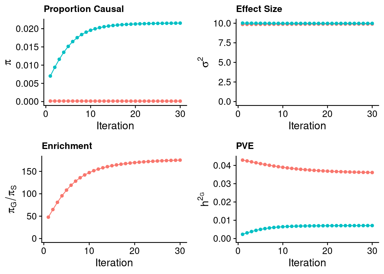
#p_pi
#p_sigma2 + theme(legend.position = "none")
#p_enrich + theme(legend.position = "none")
#p_pve + theme(legend.position = "none")

####################

#estimated group prior
estimated_group_prior <- estimated_group_prior_all[,ncol(group_prior_rec)]
-sort(-estimated_group_prior)
gene SNP
0.0215283290 0.0001229033 #estimated group prior variance
estimated_group_prior_var <- estimated_group_prior_var_all[,ncol(group_prior_var_rec)]
-sort(-estimated_group_prior_var) gene SNP
9.978117 9.896473 #estimated enrichment
estimated_enrichment <- estimated_enrichment_all[,ncol(group_prior_var_rec)]
-sort(-estimated_enrichment) gene
175.1647 #report sample size
print(sample_size)[1] 292933#report group size
print(group_size) SNP gene
8696600 9687 #estimated group PVE
estimated_group_pve <- estimated_group_pve_all[,ncol(group_prior_rec)]
-sort(-estimated_group_pve) SNP gene
0.036109819 0.007103623 #total PVE
sum(estimated_group_pve)[1] 0.04321344#attributable PVE
-sort(-estimated_group_pve/sum(estimated_group_pve)) SNP gene
0.8356154 0.1643846 Case 38 - Bilirubin with Liver - Inv-Gamma prior on variance of SNPs and genes; a=1000001, b=10000000
Load ctwas results
results_dir <- paste0("/project2/mstephens/wcrouse/ctwas_multigroup_testing/ukb-d-30780_irnt/multigroup_case38")

weight <- "/project2/compbio/predictdb/mashr_models/mashr_Liver.db"

#load information for all genes

gene_info <- data.frame(gene=as.character(), genename=as.character(), gene_type=as.character(), weight=as.character())

for (i in 1:length(weight)){
  sqlite <- RSQLite::dbDriver("SQLite")
  db = RSQLite::dbConnect(sqlite, weight[i])
  query <- function(...) RSQLite::dbGetQuery(db, ...)
  gene_info_current <- query("select gene, genename, gene_type from extra")
  RSQLite::dbDisconnect(db)

  gene_info_current$weight <- weight[i]

  gene_info <- rbind(gene_info, gene_info_current)
}

gene_info$group <- sapply(1:nrow(gene_info), function(x){paste0(unlist(strsplit(tools::file_path_sans_ext(rev(unlist(strsplit(gene_info$weight[x], "/")))[1]), "_"))[-1], collapse="_")})

gene_info$gene_id <- paste(gene_info$gene, gene_info$group, sep="|")

# #load ctwas results
# ctwas_res <- data.table::fread(paste0(results_dir, "/", analysis_id, "_ctwas.susieIrss.txt"))
#
# #make unique identifier for regions
# ctwas_res$region_tag <- paste(ctwas_res$region_tag1, ctwas_res$region_tag2, sep="_")

#load z scores for SNPs and collect sample size
load(paste0(results_dir, "/", analysis_id, "_expr_z_snp.Rd"))

sample_size <- z_snp$ss
sample_size <- as.numeric(names(which.max(table(sample_size))))

# #compute PVE for each gene/SNP
# ctwas_res$PVE = ctwas_res$susie_pip*ctwas_res$mu2/sample_size
#
# #separate gene and SNP results
# ctwas_gene_res <- ctwas_res[ctwas_res$type != "SNP", ]
# ctwas_gene_res <- data.frame(ctwas_gene_res)
# ctwas_snp_res <- ctwas_res[ctwas_res$type == "SNP", ]
# ctwas_snp_res <- data.frame(ctwas_snp_res)
#
# #add gene information to results
# ctwas_gene_res$gene_id <- sapply(ctwas_gene_res$id, function(x){unlist(strsplit(x, split="[|]"))[1]})
# ctwas_gene_res$group <- ctwas_gene_res$type
# ctwas_gene_res$alt_name <- paste0(ctwas_gene_res$gene_id, "|", ctwas_gene_res$group)
#
# ctwas_gene_res$genename <- NA
# ctwas_gene_res$gene_type <- NA
#
# group_list <- unique(ctwas_gene_res$group)
#
# for (j in 1:length(group_list)){
#   print(j)
#   group <- group_list[j]
#
#   res_group_indx <- which(ctwas_gene_res$group==group)
#   gene_info_group <- gene_info[gene_info$group==group,,drop=F]
#
#   ctwas_gene_res[res_group_indx,c("genename", "gene_type")] <- gene_info_group[sapply(ctwas_gene_res$alt_name[res_group_indx], match, gene_info_group$gene_id), c("genename", "gene_type")]
# }

#add z scores to results
load(paste0(results_dir, "/", analysis_id, "_expr_z_gene.Rd"))
#ctwas_gene_res$z <- z_gene[ctwas_gene_res$id,]$z

#z_snp <- z_snp[z_snp$id %in% ctwas_snp_res$id,]
#ctwas_snp_res$z <- z_snp$z[match(ctwas_snp_res$id, z_snp$id)]

# #merge gene and snp results with added information
# ctwas_snp_res$gene_id=NA
# ctwas_snp_res$group="SNP"
# ctwas_snp_res$alt_name=NA
# ctwas_snp_res$genename=NA
# ctwas_snp_res$gene_type=NA
#
# ctwas_res <- rbind(ctwas_gene_res,
#                    ctwas_snp_res[,colnames(ctwas_gene_res)])

#get number of SNPs from s1 results; adjust for thin argument
ctwas_res_s1 <- data.table::fread(paste0(results_dir, "/", analysis_id, "_ctwas.s1.susieIrss.txt"))
n_snps <- sum(ctwas_res_s1$type=="SNP")/thin
rm(ctwas_res_s1)

# #store columns to report
# report_cols <- colnames(ctwas_gene_res)[!(colnames(ctwas_gene_res) %in% c("type", "region_tag1", "region_tag2", "cs_index", "gene_type", "z_flag", "id", "chrom", "pos", "alt_name", "gene_id"))]
# first_cols <- c("genename", "group", "region_tag")
# report_cols <- c(first_cols, report_cols[!(report_cols %in% first_cols)])
Check convergence of parameters
library(ggplot2)
library(cowplot)

load(paste0(results_dir, "/", analysis_id, "_ctwas.s2.susieIrssres.Rd"))

#estimated group prior (all iterations)
estimated_group_prior_all <- group_prior_rec
estimated_group_prior_all["SNP",] <- estimated_group_prior_all["SNP",]*thin #adjust parameter to account for thin argument

#estimated group prior variance (all iterations)
estimated_group_prior_var_all <- group_prior_var_rec

#set group size
group_size <- structure(c(n_snps, nrow(z_gene)), names=c("SNP","gene"))

#estimated group PVE (all iterations)
estimated_group_pve_all <- estimated_group_prior_var_all*estimated_group_prior_all*group_size/sample_size #check PVE calculation

#estimated enrichment of genes (all iterations)
estimated_enrichment_all <- t(sapply(rownames(estimated_group_prior_all)[rownames(estimated_group_prior_all)!="SNP"], function(x){estimated_group_prior_all[rownames(estimated_group_prior_all)==x,]/estimated_group_prior_all[rownames(estimated_group_prior_all)=="SNP"]}))

title_size <- 12

df <- data.frame(niter = rep(1:ncol(estimated_group_prior_all), nrow(estimated_group_prior_all)),
                 value = unlist(lapply(1:nrow(estimated_group_prior_all), function(x){estimated_group_prior_all[x,]})),
                 group = rep(rownames(estimated_group_prior_all), each=ncol(estimated_group_prior_all)))

groupnames_for_plots <- sapply(as.character(unique(df$group)), function(x){paste(sapply(unlist(strsplit(x, "_")), substr, start=1, stop=3), collapse="_")})

df$group <- groupnames_for_plots[df$group]
df$group <- as.factor(df$group)

p_pi <- ggplot(df, aes(x=niter, y=value, group=group)) +
  geom_line(aes(color=group)) +
  geom_point(aes(color=group)) +
  xlab("Iteration") + ylab(bquote(pi)) +
  ggtitle("Proportion Causal") +
  theme_cowplot()

p_pi <- p_pi + theme(plot.title=element_text(size=title_size)) +
  expand_limits(y=0) +
  guides(color = guide_legend(title = "Group")) + theme (legend.title = element_text(size=12, face="bold"))

df <- data.frame(niter = rep(1:ncol(estimated_group_prior_var_all), nrow(estimated_group_prior_var_all)),
                 value = unlist(lapply(1:nrow(estimated_group_prior_var_all), function(x){estimated_group_prior_var_all[x,]})),
                 group = rep(rownames(estimated_group_prior_var_all), each=ncol(estimated_group_prior_var_all)))

groupnames_for_plots <- sapply(as.character(unique(df$group)), function(x){paste(sapply(unlist(strsplit(x, "_")), substr, start=1, stop=3), collapse="_")})

df$group <- groupnames_for_plots[df$group]
df$group <- as.factor(df$group)

p_sigma2 <- ggplot(df, aes(x=niter, y=value, group=group)) +
  geom_line(aes(color=group)) +
  geom_point(aes(color=group)) +
  xlab("Iteration") + ylab(bquote(sigma^2)) +
  ggtitle("Effect Size") +
  theme_cowplot()

p_sigma2 <- p_sigma2 + theme(plot.title=element_text(size=title_size)) +
  expand_limits(y=0) +
  guides(color = guide_legend(title = "Group")) + theme (legend.title = element_text(size=12, face="bold"))

df <- data.frame(niter = rep(1:ncol(estimated_group_pve_all), nrow(estimated_group_pve_all)),
                 value = unlist(lapply(1:nrow(estimated_group_pve_all), function(x){estimated_group_pve_all[x,]})),
                 group = rep(rownames(estimated_group_pve_all), each=ncol(estimated_group_pve_all)))

groupnames_for_plots <- sapply(as.character(unique(df$group)), function(x){paste(sapply(unlist(strsplit(x, "_")), substr, start=1, stop=3), collapse="_")})

df$group <- groupnames_for_plots[df$group]
df$group <- as.factor(df$group)

p_pve <- ggplot(df, aes(x=niter, y=value, group=group)) +
  geom_line(aes(color=group)) +
  geom_point(aes(color=group)) +
  xlab("Iteration") + ylab(bquote(h^2[G])) +
  ggtitle("PVE") +
  theme_cowplot()

p_pve <- p_pve + theme(plot.title=element_text(size=title_size)) +
  expand_limits(y=0) +
  guides(color = guide_legend(title = "Group")) + theme (legend.title = element_text(size=12, face="bold"))

df <- data.frame(niter = rep(1:ncol(estimated_enrichment_all), nrow(estimated_enrichment_all)),
                 value = unlist(lapply(1:nrow(estimated_enrichment_all), function(x){estimated_enrichment_all[x,]})),
                 group = rep(rownames(estimated_enrichment_all), each=ncol(estimated_enrichment_all)))

groupnames_for_plots <- sapply(as.character(unique(df$group)), function(x){paste(sapply(unlist(strsplit(x, "_")), substr, start=1, stop=3), collapse="_")})

df$group <- groupnames_for_plots[df$group]
df$group <- as.factor(df$group)

p_enrich <- ggplot(df, aes(x=niter, y=value, group=group)) +
  geom_line(aes(color=group)) +
  geom_point(aes(color=group)) +
  xlab("Iteration") + ylab(bquote(pi[G]/pi[S])) +
  ggtitle("Enrichment") +
  theme_cowplot()

p_enrich <- p_enrich + theme(plot.title=element_text(size=title_size)) +
  expand_limits(y=0) +
  guides(color = guide_legend(title = "Group")) + theme (legend.title = element_text(size=12, face="bold"))

plot_grid(p_pi + theme(legend.position = "none"),
          p_sigma2 + theme(legend.position = "none"),
          p_enrich + theme(legend.position = "none"),
          p_pve+ theme(legend.position = "none"))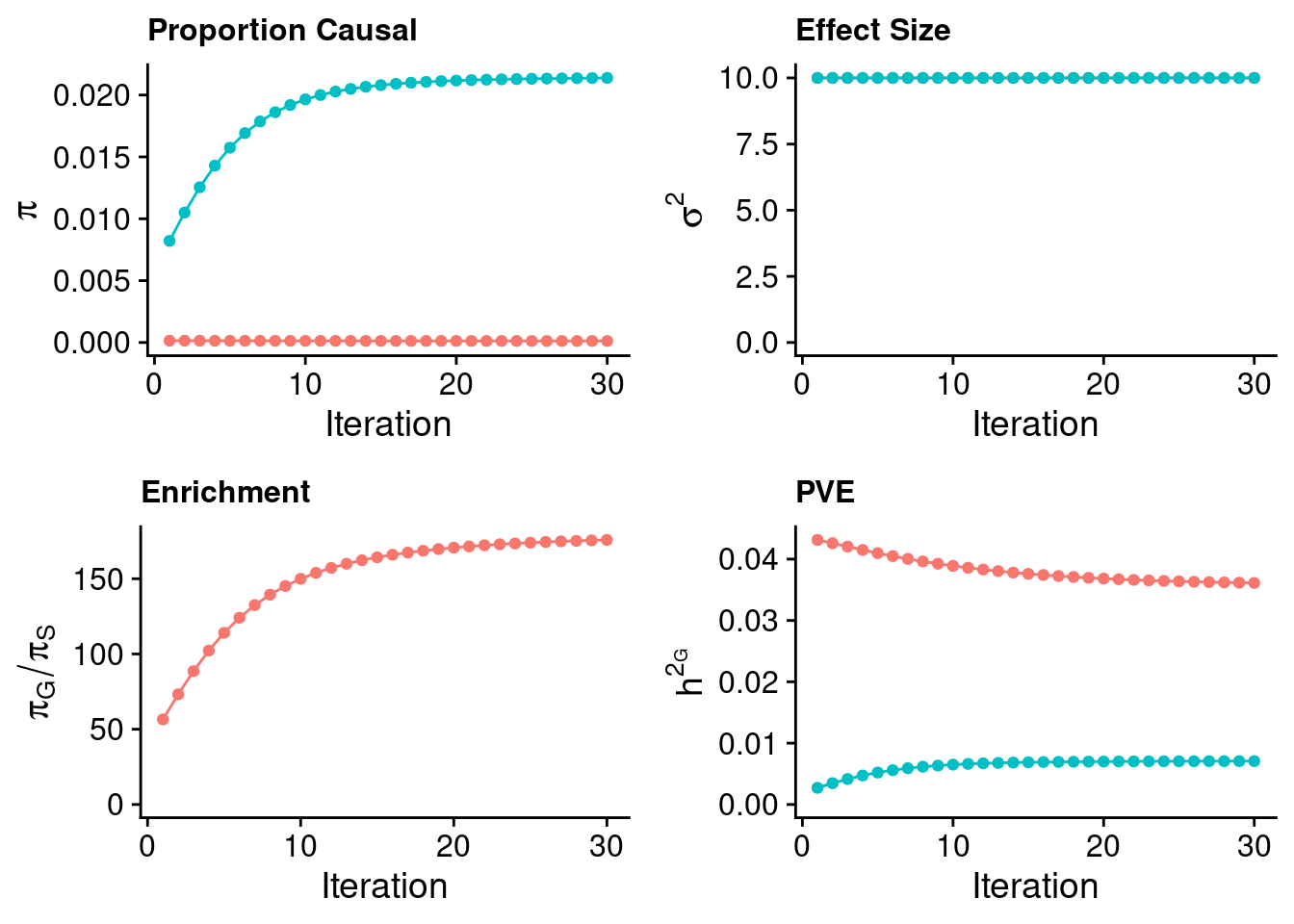
#p_pi
#p_sigma2 + theme(legend.position = "none")
#p_enrich + theme(legend.position = "none")
#p_pve + theme(legend.position = "none")

####################

#estimated group prior
estimated_group_prior <- estimated_group_prior_all[,ncol(group_prior_rec)]
-sort(-estimated_group_prior)
gene SNP
0.0213809018 0.0001216473 #estimated group prior variance
estimated_group_prior_var <- estimated_group_prior_var_all[,ncol(group_prior_var_rec)]
-sort(-estimated_group_prior_var) gene SNP
9.999914 9.999574 #estimated enrichment
estimated_enrichment <- estimated_enrichment_all[,ncol(group_prior_var_rec)]
-sort(-estimated_enrichment) gene
175.7614 #report sample size
print(sample_size)[1] 292933#report group size
print(group_size) SNP gene
8696600 9687 #estimated group PVE
estimated_group_pve <- estimated_group_pve_all[,ncol(group_prior_rec)]
-sort(-estimated_group_pve) SNP gene
0.036113143 0.007070388 #total PVE
sum(estimated_group_pve)[1] 0.04318353#attributable PVE
-sort(-estimated_group_pve/sum(estimated_group_pve)) SNP gene
0.8362712 0.1637288
sessionInfo()R version 4.1.0 (2021-05-18)
Platform: x86_64-pc-linux-gnu (64-bit)
Running under: CentOS Linux 7 (Core)
Matrix products: default
BLAS: /software/R-4.1.0-no-openblas-el7-x86_64/lib64/R/lib/libRblas.so
LAPACK: /software/R-4.1.0-no-openblas-el7-x86_64/lib64/R/lib/libRlapack.so
locale:
[1] LC_CTYPE=en_US.UTF-8 LC_NUMERIC=C LC_TIME=C
[4] LC_COLLATE=C LC_MONETARY=C LC_MESSAGES=C
[7] LC_PAPER=C LC_NAME=C LC_ADDRESS=C
[10] LC_TELEPHONE=C LC_MEASUREMENT=C LC_IDENTIFICATION=C
attached base packages:
[1] stats graphics grDevices utils datasets methods base
other attached packages:
[1] cowplot_1.1.1 ggplot2_3.4.0 workflowr_1.7.0
loaded via a namespace (and not attached):
[1] tidyselect_1.2.0 xfun_0.35 bslib_0.4.1 colorspace_2.0-3
[5] vctrs_0.5.1 generics_0.1.3 htmltools_0.5.4 yaml_2.3.6
[9] utf8_1.2.2 blob_1.2.3 rlang_1.0.6 jquerylib_0.1.4
[13] later_1.3.0 pillar_1.8.1 withr_2.5.0 glue_1.6.2
[17] DBI_1.1.3 bit64_4.0.5 lifecycle_1.0.3 stringr_1.5.0
[21] munsell_0.5.0 gtable_0.3.1 evaluate_0.18 memoise_2.0.1
[25] labeling_0.4.2 knitr_1.41 callr_3.7.3 fastmap_1.1.0
[29] httpuv_1.6.6 ps_1.7.2 fansi_1.0.3 highr_0.9
[33] Rcpp_1.0.9 promises_1.2.0.1 scales_1.2.1 cachem_1.0.6
[37] jsonlite_1.8.4 farver_2.1.1 fs_1.5.2 bit_4.0.5
[41] digest_0.6.31 stringi_1.7.8 processx_3.8.0 dplyr_1.0.10
[45] getPass_0.2-2 rprojroot_2.0.3 grid_4.1.0 cli_3.4.1
[49] tools_4.1.0 magrittr_2.0.3 sass_0.4.4 tibble_3.1.8
[53] RSQLite_2.2.19 whisker_0.4.1 pkgconfig_2.0.3 data.table_1.14.6
[57] assertthat_0.2.1 rmarkdown_2.18 httr_1.4.4 rstudioapi_0.14
[61] R6_2.5.1 git2r_0.30.1 compiler_4.1.0