Testosterone (quantile) - Liver
wesleycrouse
2021-09-09
Last updated: 2021-09-09
Checks: 6 1
Knit directory: ctwas_applied/
This reproducible R Markdown analysis was created with workflowr (version 1.6.2). The Checks tab describes the reproducibility checks that were applied when the results were created. The Past versions tab lists the development history.
The R Markdown file has unstaged changes. To know which version of the R Markdown file created these results, you’ll want to first commit it to the Git repo. If you’re still working on the analysis, you can ignore this warning. When you’re finished, you can run wflow_publish to commit the R Markdown file and build the HTML.
Great job! The global environment was empty. Objects defined in the global environment can affect the analysis in your R Markdown file in unknown ways. For reproduciblity it’s best to always run the code in an empty environment.
The command set.seed(20210726) was run prior to running the code in the R Markdown file. Setting a seed ensures that any results that rely on randomness, e.g. subsampling or permutations, are reproducible.
Great job! Recording the operating system, R version, and package versions is critical for reproducibility.
Nice! There were no cached chunks for this analysis, so you can be confident that you successfully produced the results during this run.
Great job! Using relative paths to the files within your workflowr project makes it easier to run your code on other machines.
Great! You are using Git for version control. Tracking code development and connecting the code version to the results is critical for reproducibility.
The results in this page were generated with repository version 59e5f4d. See the Past versions tab to see a history of the changes made to the R Markdown and HTML files.
Note that you need to be careful to ensure that all relevant files for the analysis have been committed to Git prior to generating the results (you can use wflow_publish or wflow_git_commit). workflowr only checks the R Markdown file, but you know if there are other scripts or data files that it depends on. Below is the status of the Git repository when the results were generated:
Unstaged changes:
    Modified:   analysis/ukb-d-30500_irnt_Liver.Rmd
    Modified:   analysis/ukb-d-30600_irnt_Liver.Rmd
    Modified:   analysis/ukb-d-30610_irnt_Liver.Rmd
    Modified:   analysis/ukb-d-30620_irnt_Liver.Rmd
    Modified:   analysis/ukb-d-30630_irnt_Liver.Rmd
    Modified:   analysis/ukb-d-30640_irnt_Liver.Rmd
    Modified:   analysis/ukb-d-30650_irnt_Liver.Rmd
    Modified:   analysis/ukb-d-30660_irnt_Liver.Rmd
    Modified:   analysis/ukb-d-30670_irnt_Liver.Rmd
    Modified:   analysis/ukb-d-30680_irnt_Liver.Rmd
    Modified:   analysis/ukb-d-30690_irnt_Liver.Rmd
    Modified:   analysis/ukb-d-30700_irnt_Liver.Rmd
    Modified:   analysis/ukb-d-30710_irnt_Liver.Rmd
    Modified:   analysis/ukb-d-30720_irnt_Liver.Rmd
    Modified:   analysis/ukb-d-30730_irnt_Liver.Rmd
    Modified:   analysis/ukb-d-30740_irnt_Liver.Rmd
    Modified:   analysis/ukb-d-30750_irnt_Liver.Rmd
    Modified:   analysis/ukb-d-30760_irnt_Liver.Rmd
    Modified:   analysis/ukb-d-30770_irnt_Liver.Rmd
    Modified:   analysis/ukb-d-30780_irnt_Liver.Rmd
    Modified:   analysis/ukb-d-30790_irnt_Liver.Rmd
    Modified:   analysis/ukb-d-30800_irnt_Liver.Rmd
    Modified:   analysis/ukb-d-30810_irnt_Liver.Rmd
    Modified:   analysis/ukb-d-30820_irnt_Liver.Rmd
    Modified:   analysis/ukb-d-30830_irnt_Liver.Rmd
    Modified:   analysis/ukb-d-30840_irnt_Liver.Rmd
    Modified:   analysis/ukb-d-30850_irnt_Liver.Rmd
Note that any generated files, e.g. HTML, png, CSS, etc., are not included in this status report because it is ok for generated content to have uncommitted changes.
These are the previous versions of the repository in which changes were made to the R Markdown (analysis/ukb-d-30850_irnt_Liver.Rmd) and HTML (docs/ukb-d-30850_irnt_Liver.html) files. If you’ve configured a remote Git repository (see ?wflow_git_remote), click on the hyperlinks in the table below to view the files as they were in that past version.
| File | Version | Author | Date | Message |
|---|---|---|---|---|
| Rmd | cbf7408 | wesleycrouse | 2021-09-08 | adding enrichment to reports |
| html | cbf7408 | wesleycrouse | 2021-09-08 | adding enrichment to reports |
| Rmd | 4970e3e | wesleycrouse | 2021-09-08 | updating reports |
| html | 4970e3e | wesleycrouse | 2021-09-08 | updating reports |
| Rmd | dfd2b5f | wesleycrouse | 2021-09-07 | regenerating reports |
| html | dfd2b5f | wesleycrouse | 2021-09-07 | regenerating reports |
| Rmd | 61b53b3 | wesleycrouse | 2021-09-06 | updated PVE calculation |
| html | 61b53b3 | wesleycrouse | 2021-09-06 | updated PVE calculation |
| Rmd | 837dd01 | wesleycrouse | 2021-09-01 | adding additional fixedsigma report |
| Rmd | d0a5417 | wesleycrouse | 2021-08-30 | adding new reports to the index |
| Rmd | 0922de7 | wesleycrouse | 2021-08-18 | updating all reports with locus plots |
| html | 0922de7 | wesleycrouse | 2021-08-18 | updating all reports with locus plots |
| html | 1c62980 | wesleycrouse | 2021-08-11 | Updating reports |
| Rmd | 5981e80 | wesleycrouse | 2021-08-11 | Adding more reports |
| html | 5981e80 | wesleycrouse | 2021-08-11 | Adding more reports |
| Rmd | 05a98b7 | wesleycrouse | 2021-08-07 | adding additional results |
| html | 05a98b7 | wesleycrouse | 2021-08-07 | adding additional results |
| html | 03e541c | wesleycrouse | 2021-07-29 | Cleaning up report generation |
| Rmd | 276893d | wesleycrouse | 2021-07-29 | Updating reports |
| html | 276893d | wesleycrouse | 2021-07-29 | Updating reports |
Overview
These are the results of a ctwas analysis of the UK Biobank trait Testosterone (quantile) using Liver gene weights.
The GWAS was conducted by the Neale Lab, and the biomarker traits we analyzed are discussed here. Summary statistics were obtained from IEU OpenGWAS using GWAS ID: ukb-d-30850_irnt. Results were obtained from from IEU rather than Neale Lab because they are in a standardard format (GWAS VCF). Note that 3 of the 34 biomarker traits were not available from IEU and were excluded from analysis.
The weights are mashr GTEx v8 models on Liver eQTL obtained from PredictDB. We performed a full harmonization of the variants, including recovering strand ambiguous variants. This procedure is discussed in a separate document. (TO-DO: add report that describes harmonization)
LD matrices were computed from a 10% subset of Neale lab subjects. Subjects were matched using the plate and well information from genotyping. We included only biallelic variants with MAF>0.01 in the original Neale Lab GWAS. (TO-DO: add more details [number of subjects, variants, etc])
Weight QC
TO-DO: add enhanced QC reporting (total number of weights, why each variant was missing for all genes)
qclist_all <- list()

qc_files <- paste0(results_dir, "/", list.files(results_dir, pattern="exprqc.Rd"))

for (i in 1:length(qc_files)){
  load(qc_files[i])
  chr <- unlist(strsplit(rev(unlist(strsplit(qc_files[i], "_")))[1], "[.]"))[1]
  qclist_all[[chr]] <- cbind(do.call(rbind, lapply(qclist,unlist)), as.numeric(substring(chr,4)))
}

qclist_all <- data.frame(do.call(rbind, qclist_all))
colnames(qclist_all)[ncol(qclist_all)] <- "chr"

rm(qclist, wgtlist, z_gene_chr)

#number of imputed weights
nrow(qclist_all)
[1] 10901#number of imputed weights by chromosome
table(qclist_all$chr)
   1    2    3    4    5    6    7    8    9   10   11   12   13   14   15
1070  768  652  417  494  611  548  408  405  434  634  629  195  365  354
  16   17   18   19   20   21   22
 526  663  160  859  306  114  289
#proportion of imputed weights without missing variants
mean(qclist_all$nmiss==0)[1] 0.8366205Load ctwas results
#load ctwas results
ctwas_res <- data.table::fread(paste0(results_dir, "/", analysis_id, "_ctwas.susieIrss.txt"))

#make unique identifier for regions
ctwas_res$region_tag <- paste(ctwas_res$region_tag1, ctwas_res$region_tag2, sep="_")

#compute PVE for each gene/SNP
ctwas_res$PVE = ctwas_res$susie_pip*ctwas_res$mu2/sample_size #check PVE calculation

#separate gene and SNP results
ctwas_gene_res <- ctwas_res[ctwas_res$type == "gene", ]
ctwas_gene_res <- data.frame(ctwas_gene_res)
ctwas_snp_res <- ctwas_res[ctwas_res$type == "SNP", ]
ctwas_snp_res <- data.frame(ctwas_snp_res)

#add gene information to results
sqlite <- RSQLite::dbDriver("SQLite")
db = RSQLite::dbConnect(sqlite, paste0("/project2/compbio/predictdb/mashr_models/mashr_", weight, ".db"))
query <- function(...) RSQLite::dbGetQuery(db, ...)
gene_info <- query("select gene, genename from extra")
gene_info <- query("select gene, genename, gene_type from extra")
RSQLite::dbDisconnect(db)

ctwas_gene_res <- cbind(ctwas_gene_res, gene_info[sapply(ctwas_gene_res$id, match, gene_info$gene), c("genename", "gene_type")])

#add z score to results
load(paste0(results_dir, "/", analysis_id, "_expr_z_gene.Rd"))
ctwas_gene_res$z <- z_gene[ctwas_gene_res$id,]$z

#load(paste0(results_dir, "/", analysis_id, "_expr_z_snp.Rd")) #for new version, stored after harmonization
z_snp <- readRDS(paste0(results_dir, "/", trait_id, ".RDS")) #for old version, unharmonized

z_snp <- z_snp[z_snp$id %in% ctwas_snp_res$id,] #subset snps to those included in analysis, note some are duplicated, need to match which allele was used
ctwas_snp_res$z <- z_snp$z[match(ctwas_snp_res$id, z_snp$id)] #for duplicated snps, this arbitrarily uses the first allele
ctwas_snp_res$z_flag <- as.numeric(ctwas_snp_res$id %in% z_snp$id[duplicated(z_snp$id)]) #mark the unclear z scores, flag=1

#formatting and rounding for tables
ctwas_gene_res$z <- round(ctwas_gene_res$z,2)
ctwas_snp_res$z <- round(ctwas_snp_res$z,2)
ctwas_gene_res$susie_pip <- round(ctwas_gene_res$susie_pip,3)
ctwas_snp_res$susie_pip <- round(ctwas_snp_res$susie_pip,3)
ctwas_gene_res$mu2 <- round(ctwas_gene_res$mu2,2)
ctwas_snp_res$mu2 <- round(ctwas_snp_res$mu2,2)
ctwas_gene_res$PVE <- signif(ctwas_gene_res$PVE, 2)
ctwas_snp_res$PVE <- signif(ctwas_snp_res$PVE, 2)

#merge gene and snp results with added information
ctwas_gene_res$z_flag=NA
ctwas_snp_res$genename=NA
ctwas_snp_res$gene_type=NA

ctwas_res <- rbind(ctwas_gene_res,
                   ctwas_snp_res[,colnames(ctwas_gene_res)])

#store columns to report
report_cols <- colnames(ctwas_gene_res)[!(colnames(ctwas_gene_res) %in% c("type", "region_tag1", "region_tag2", "cs_index", "gene_type", "z_flag", "id", "chrom", "pos"))]
first_cols <- c("genename", "region_tag")
report_cols <- c(first_cols, report_cols[!(report_cols %in% first_cols)])

report_cols_snps <- c("id", report_cols[-1])

#get number of SNPs from s1 results; adjust for thin
ctwas_res_s1 <- data.table::fread(paste0(results_dir, "/", analysis_id, "_ctwas.s1.susieIrss.txt"))
n_snps <- sum(ctwas_res_s1$type=="SNP")/thin
rm(ctwas_res_s1)
Check convergence of parameters
library(ggplot2)
library(cowplot)
********************************************************Note: As of version 1.0.0, cowplot does not change the default ggplot2 theme anymore. To recover the previous behavior, execute:
theme_set(theme_cowplot())********************************************************load(paste0(results_dir, "/", analysis_id, "_ctwas.s2.susieIrssres.Rd"))
df <- data.frame(niter = rep(1:ncol(group_prior_rec), 2),
value = c(group_prior_rec[1,], group_prior_rec[2,]),
group = rep(c("Gene", "SNP"), each = ncol(group_prior_rec)))
df$group <- as.factor(df$group)
df$value[df$group=="SNP"] <- df$value[df$group=="SNP"]*thin #adjust parameter to account for thin argument
p_pi <- ggplot(df, aes(x=niter, y=value, group=group)) +
geom_line(aes(color=group)) +
geom_point(aes(color=group)) +
xlab("Iteration") + ylab(bquote(pi)) +
ggtitle("Prior mean") +
theme_cowplot()
df <- data.frame(niter = rep(1:ncol(group_prior_var_rec), 2),
value = c(group_prior_var_rec[1,], group_prior_var_rec[2,]),
group = rep(c("Gene", "SNP"), each = ncol(group_prior_var_rec)))
df$group <- as.factor(df$group)
p_sigma2 <- ggplot(df, aes(x=niter, y=value, group=group)) +
geom_line(aes(color=group)) +
geom_point(aes(color=group)) +
xlab("Iteration") + ylab(bquote(sigma^2)) +
ggtitle("Prior variance") +
theme_cowplot()
plot_grid(p_pi, p_sigma2)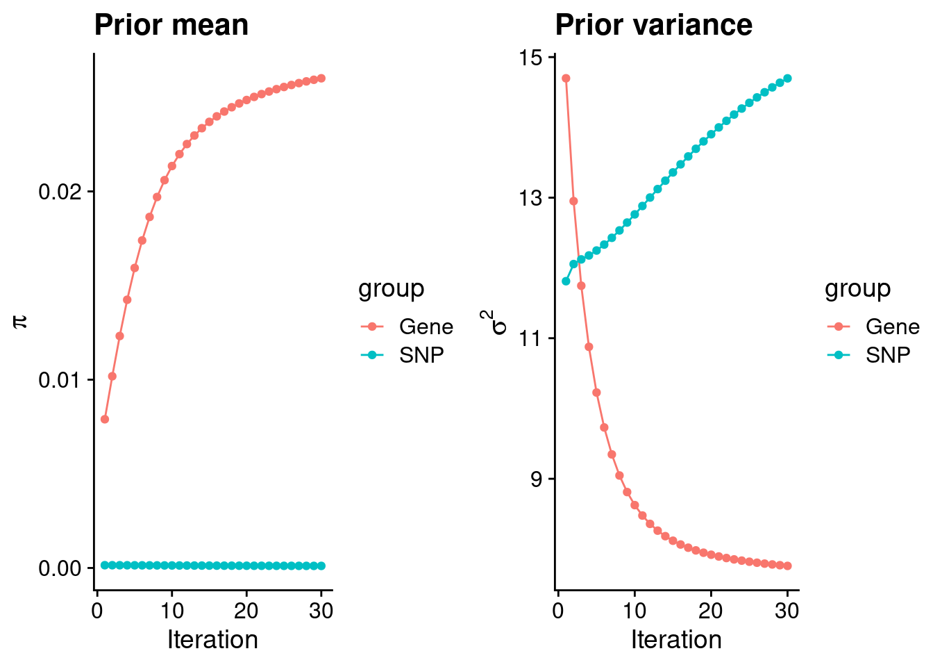
| Version | Author | Date |
|---|---|---|
| dfd2b5f | wesleycrouse | 2021-09-07 |
#estimated group prior
estimated_group_prior <- group_prior_rec[,ncol(group_prior_rec)]
names(estimated_group_prior) <- c("gene", "snp")
estimated_group_prior["snp"] <- estimated_group_prior["snp"]*thin #adjust parameter to account for thin argument
print(estimated_group_prior)
gene snp
0.026008197 0.000109673 #estimated group prior variance
estimated_group_prior_var <- group_prior_var_rec[,ncol(group_prior_var_rec)]
names(estimated_group_prior_var) <- c("gene", "snp")
print(estimated_group_prior_var) gene snp
7.76021 14.69737 #report sample size
print(sample_size)[1] 312102#report group size
group_size <- c(nrow(ctwas_gene_res), n_snps)
print(group_size)[1] 10901 8697330#estimated group PVE
estimated_group_pve <- estimated_group_prior_var*estimated_group_prior*group_size/sample_size #check PVE calculation
names(estimated_group_pve) <- c("gene", "snp")
print(estimated_group_pve) gene snp
0.007049421 0.044918881 #compare sum(PIP*mu2/sample_size) with above PVE calculation
c(sum(ctwas_gene_res$PVE),sum(ctwas_snp_res$PVE))[1] 0.03895237 0.41612045Genes with highest PIPs
#distribution of PIPs
hist(ctwas_gene_res$susie_pip, xlim=c(0,1), main="Distribution of Gene PIPs")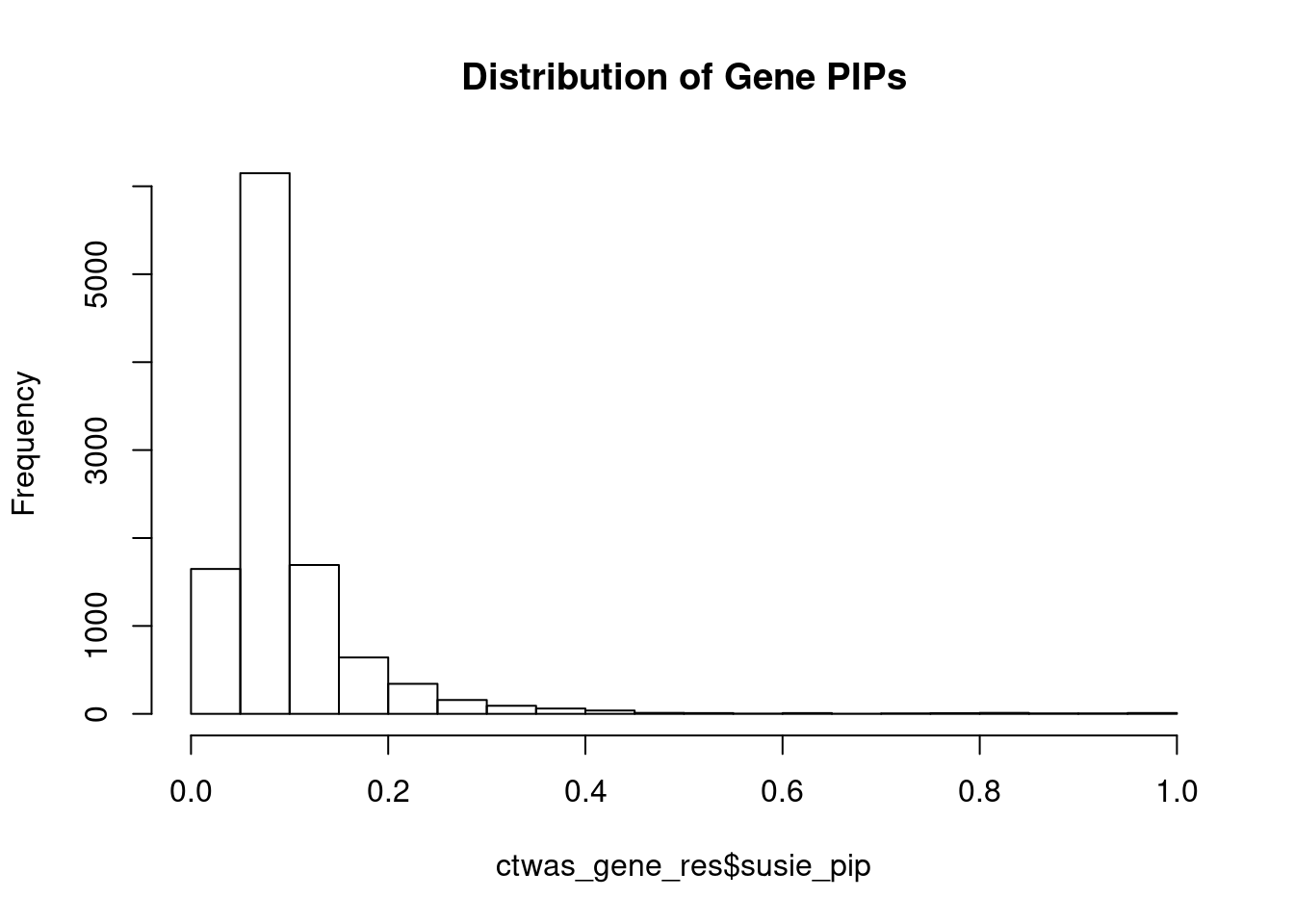
| Version | Author | Date |
|---|---|---|
| dfd2b5f | wesleycrouse | 2021-09-07 |
#genes with PIP>0.8 or 20 highest PIPs
head(ctwas_gene_res[order(-ctwas_gene_res$susie_pip),report_cols], max(sum(ctwas_gene_res$susie_pip>0.8), 20))
genename region_tag susie_pip mu2 PVE z
11889 RP11-327J17.2 15_46 0.991 23.18 7.4e-05 -3.80
1488 MIEF1 22_16 0.987 31.24 9.9e-05 -5.79
1231 PABPC4 1_24 0.982 29.40 9.3e-05 5.44
11297 HLA-B 6_25 0.982 27.72 8.7e-05 -6.09
11797 URB1-AS1 21_13 0.981 20.56 6.5e-05 -4.50
2678 TFEB 6_32 0.980 24.16 7.6e-05 5.08
6126 VENTX 10_85 0.975 25.46 8.0e-05 5.17
9383 PCP4 21_19 0.971 20.00 6.2e-05 4.36
6214 NADK2 5_24 0.953 19.55 6.0e-05 -4.24
10303 UGT2B17 4_48 0.952 37.75 1.2e-04 7.24
3150 KMT2A 11_71 0.937 29.88 9.0e-05 -5.59
191 CEP68 2_42 0.929 21.41 6.4e-05 -4.53
8803 DLEU1 13_21 0.924 22.87 6.8e-05 -4.76
2204 AKNA 9_59 0.923 20.06 5.9e-05 -4.32
5799 SLC22A3 6_104 0.920 27.66 8.2e-05 5.36
4085 JUND 19_14 0.890 26.68 7.6e-05 -5.31
11281 RP3-413H6.2 6_11 0.886 18.04 5.1e-05 3.93
3619 PEPD 19_23 0.861 20.73 5.7e-05 4.56
3641 SLC17A1 6_20 0.857 18.15 5.0e-05 4.00
11279 AC098828.2 2_12 0.851 22.06 6.0e-05 -4.94
7656 CATSPER2 15_16 0.850 39.98 1.1e-04 -7.43
11632 LINC01612 4_111 0.848 20.46 5.6e-05 -4.50
1235 USP48 1_15 0.847 18.21 4.9e-05 -3.90
9052 RMI1 9_41 0.845 30.07 8.1e-05 -5.72
2258 FBXW4 10_65 0.843 25.29 6.8e-05 -4.34
10908 AS3MT 10_66 0.834 56.44 1.5e-04 7.85
7503 ZNF219 14_1 0.834 17.18 4.6e-05 -3.86
6509 NTAN1 16_15 0.830 19.82 5.3e-05 -4.33
12051 LINC00672 17_23 0.828 18.18 4.8e-05 -4.00
9404 PTTG1IP 21_23 0.822 18.00 4.7e-05 3.86
8767 MLXIP 12_75 0.818 19.33 5.1e-05 -3.97Genes with largest effect sizes
#plot PIP vs effect size
plot(ctwas_gene_res$susie_pip, ctwas_gene_res$mu2, xlab="PIP", ylab="mu^2", main="Gene PIPs vs Effect Size")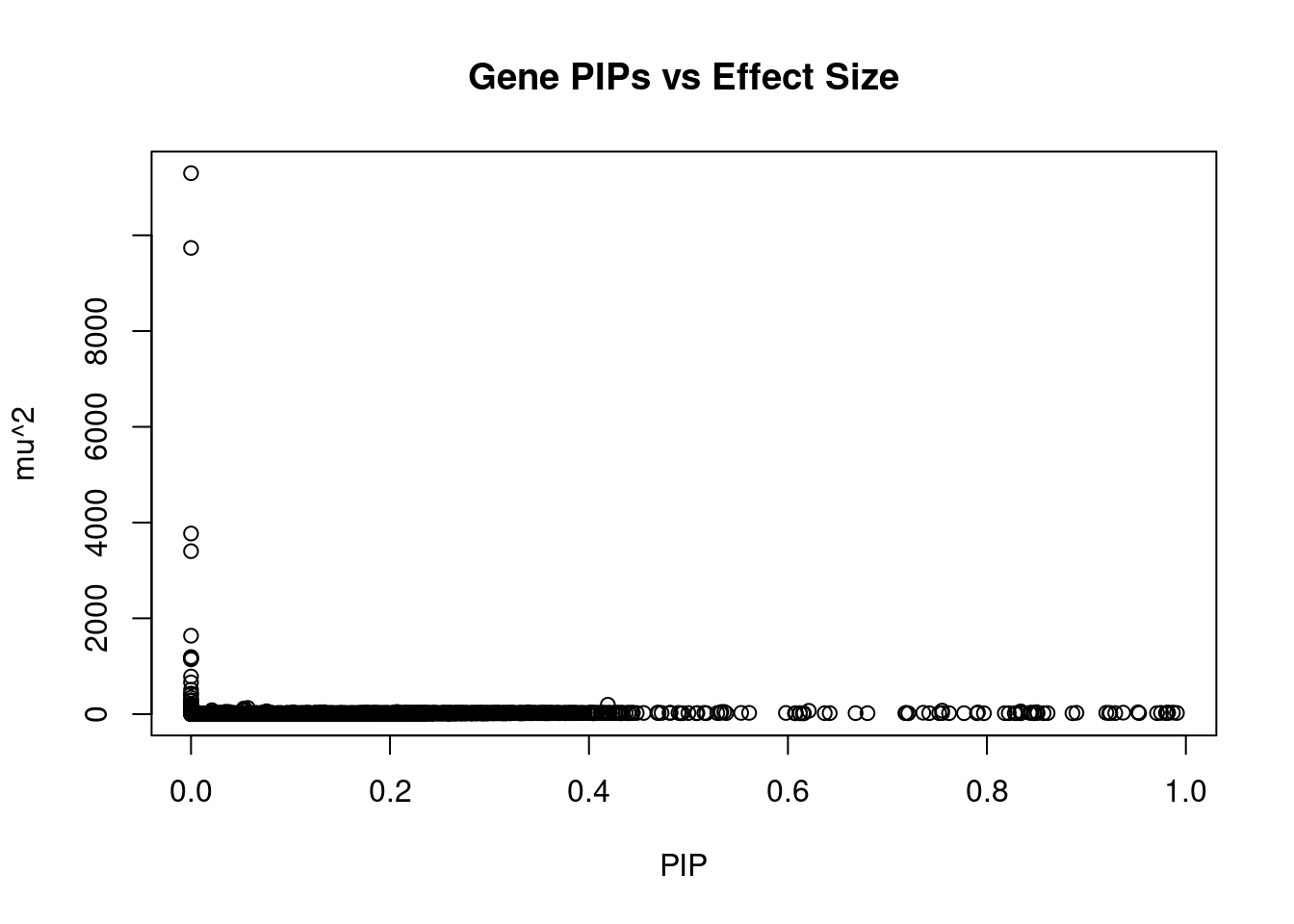
| Version | Author | Date |
|---|---|---|
| dfd2b5f | wesleycrouse | 2021-09-07 |
#genes with 20 largest effect sizes
head(ctwas_gene_res[order(-ctwas_gene_res$mu2),report_cols],20)
genename region_tag susie_pip mu2 PVE z
5389 RPS11 19_34 0 11298.20 0.0e+00 -4.69
1227 FLT3LG 19_34 0 9736.31 0.0e+00 3.77
5393 RCN3 19_34 0 3771.45 0.0e+00 5.85
1931 FCGRT 19_34 0 3402.69 0.0e+00 4.47
3804 PRRG2 19_34 0 1637.00 0.0e+00 1.71
11199 LINC00271 6_89 0 1191.15 0.0e+00 2.02
3805 SCAF1 19_34 0 1173.94 0.0e+00 3.98
3803 PRMT1 19_34 0 1157.04 0.0e+00 3.67
3802 IRF3 19_34 0 1143.07 0.0e+00 3.98
1940 SLC17A7 19_34 0 785.22 0.0e+00 -0.22
6880 TNFSF13 17_7 0 662.33 0.0e+00 34.29
3991 ATP1B2 17_7 0 509.63 1.1e-15 -28.39
6883 EIF4A1 17_7 0 428.99 0.0e+00 -19.79
4604 AHI1 6_89 0 414.41 0.0e+00 1.13
1932 PIH1D1 19_34 0 343.22 0.0e+00 -0.53
11399 TNFSF12 17_7 0 288.75 0.0e+00 16.61
6881 SENP3 17_7 0 283.01 2.8e-13 12.96
10291 CTC-301O7.4 19_34 0 277.27 0.0e+00 -0.57
5313 SAT2 17_7 0 208.24 1.5e-19 -13.77
5311 WRAP53 17_7 0 204.81 8.2e-13 -15.51Genes with highest PVE
#genes with 20 highest pve
head(ctwas_gene_res[order(-ctwas_gene_res$PVE),report_cols],20)
genename region_tag susie_pip mu2 PVE z
10495 PRMT6 1_66 0.419 195.20 2.6e-04 -9.52
7355 BRI3 7_60 0.755 72.10 1.7e-04 -9.22
10908 AS3MT 10_66 0.834 56.44 1.5e-04 7.85
8284 RBKS 2_16 0.621 68.48 1.4e-04 -10.02
10303 UGT2B17 4_48 0.952 37.75 1.2e-04 7.24
7656 CATSPER2 15_16 0.850 39.98 1.1e-04 -7.43
1488 MIEF1 22_16 0.987 31.24 9.9e-05 -5.79
1231 PABPC4 1_24 0.982 29.40 9.3e-05 5.44
3150 KMT2A 11_71 0.937 29.88 9.0e-05 -5.59
4925 IFT172 2_16 0.791 34.84 8.8e-05 -7.78
11297 HLA-B 6_25 0.982 27.72 8.7e-05 -6.09
5799 SLC22A3 6_104 0.920 27.66 8.2e-05 5.36
9052 RMI1 9_41 0.845 30.07 8.1e-05 -5.72
6126 VENTX 10_85 0.975 25.46 8.0e-05 5.17
9573 SLC22A10 11_35 0.536 44.74 7.7e-05 7.17
2678 TFEB 6_32 0.980 24.16 7.6e-05 5.08
4085 JUND 19_14 0.890 26.68 7.6e-05 -5.31
1343 SIRT1 10_44 0.533 44.04 7.5e-05 6.99
11889 RP11-327J17.2 15_46 0.991 23.18 7.4e-05 -3.80
2258 FBXW4 10_65 0.843 25.29 6.8e-05 -4.34Genes with largest z scores
#genes with 20 largest z scores
head(ctwas_gene_res[order(-abs(ctwas_gene_res$z)),report_cols],20)
genename region_tag susie_pip mu2 PVE z
6880 TNFSF13 17_7 0.000 662.33 0.0e+00 34.29
3991 ATP1B2 17_7 0.000 509.63 1.1e-15 -28.39
6883 EIF4A1 17_7 0.000 428.99 0.0e+00 -19.79
11399 TNFSF12 17_7 0.000 288.75 0.0e+00 16.61
9477 DNAH2 17_7 0.000 193.10 0.0e+00 16.09
5311 WRAP53 17_7 0.000 204.81 8.2e-13 -15.51
5313 SAT2 17_7 0.000 208.24 1.5e-19 -13.77
6881 SENP3 17_7 0.000 283.01 2.8e-13 12.96
11526 GS1-259H13.2 7_61 0.057 128.99 2.4e-05 12.40
2887 NRBP1 2_16 0.021 80.67 5.5e-06 -11.91
2139 PTCD1 7_61 0.054 117.14 2.0e-05 11.82
6814 CPSF4 7_61 0.053 115.98 2.0e-05 11.76
8284 RBKS 2_16 0.621 68.48 1.4e-04 -10.02
10495 PRMT6 1_66 0.419 195.20 2.6e-04 -9.52
10415 ZNF789 7_61 0.055 74.23 1.3e-05 9.35
7355 BRI3 7_60 0.755 72.10 1.7e-04 -9.22
10851 UGT2B11 4_48 0.000 168.58 8.8e-08 -8.69
4936 SLC5A6 2_16 0.038 46.26 5.6e-06 -8.35
2611 MCM9 6_79 0.076 59.31 1.4e-05 8.27
4941 ATRAID 2_16 0.035 44.64 5.0e-06 8.27Comparing z scores and PIPs
#set nominal signifiance threshold for z scores
alpha <- 0.05

#bonferroni adjusted threshold for z scores
sig_thresh <- qnorm(1-(alpha/nrow(ctwas_gene_res)/2), lower=T)

#Q-Q plot for z scores
obs_z <- ctwas_gene_res$z[order(ctwas_gene_res$z)]
exp_z <- qnorm((1:nrow(ctwas_gene_res))/nrow(ctwas_gene_res))

plot(exp_z, obs_z, xlab="Expected z", ylab="Observed z", main="Gene z score Q-Q plot")
abline(a=0,b=1)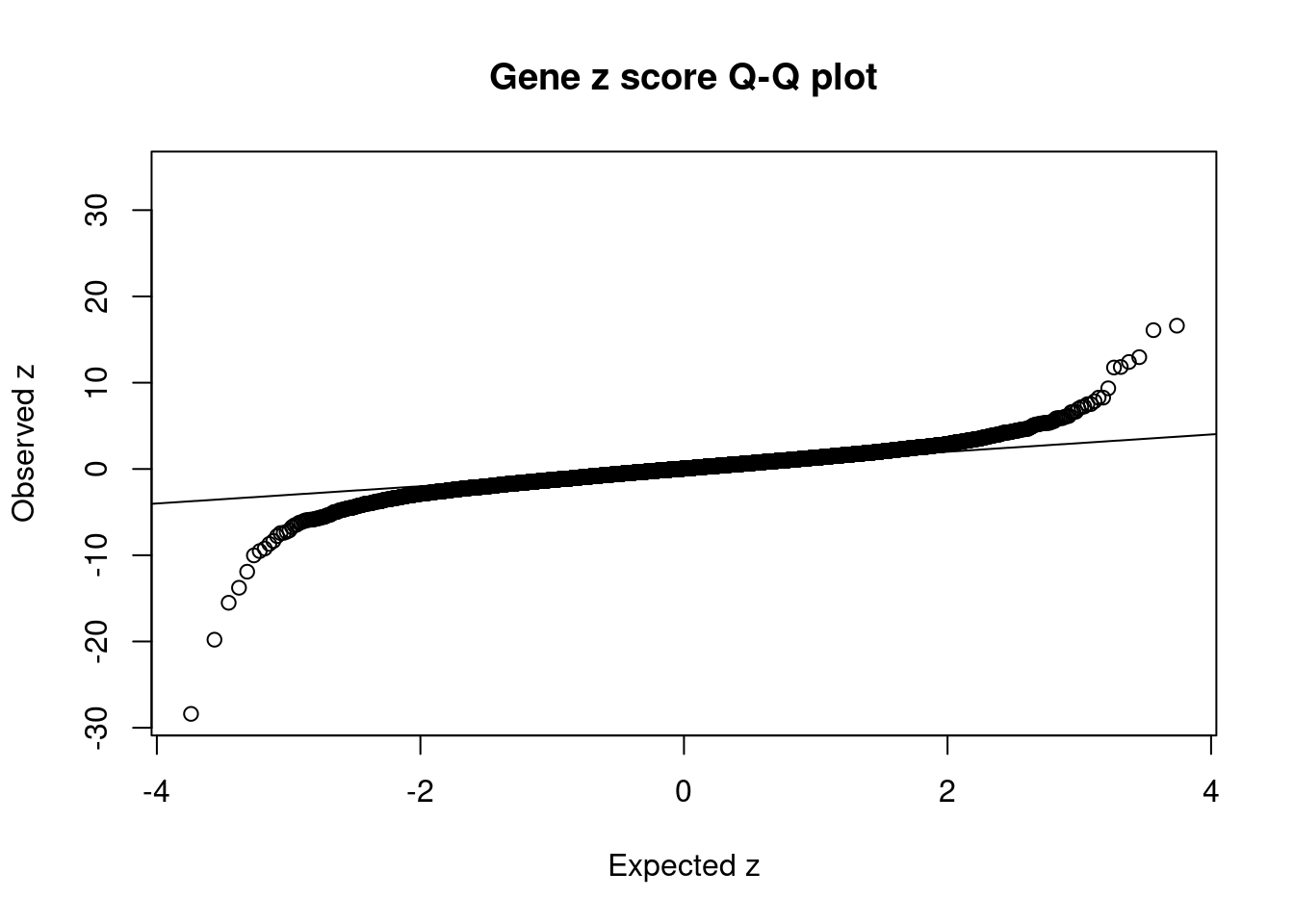
| Version | Author | Date |
|---|---|---|
| dfd2b5f | wesleycrouse | 2021-09-07 |
#plot z score vs PIP
plot(abs(ctwas_gene_res$z), ctwas_gene_res$susie_pip, xlab="abs(z)", ylab="PIP")
abline(v=sig_thresh, col="red", lty=2)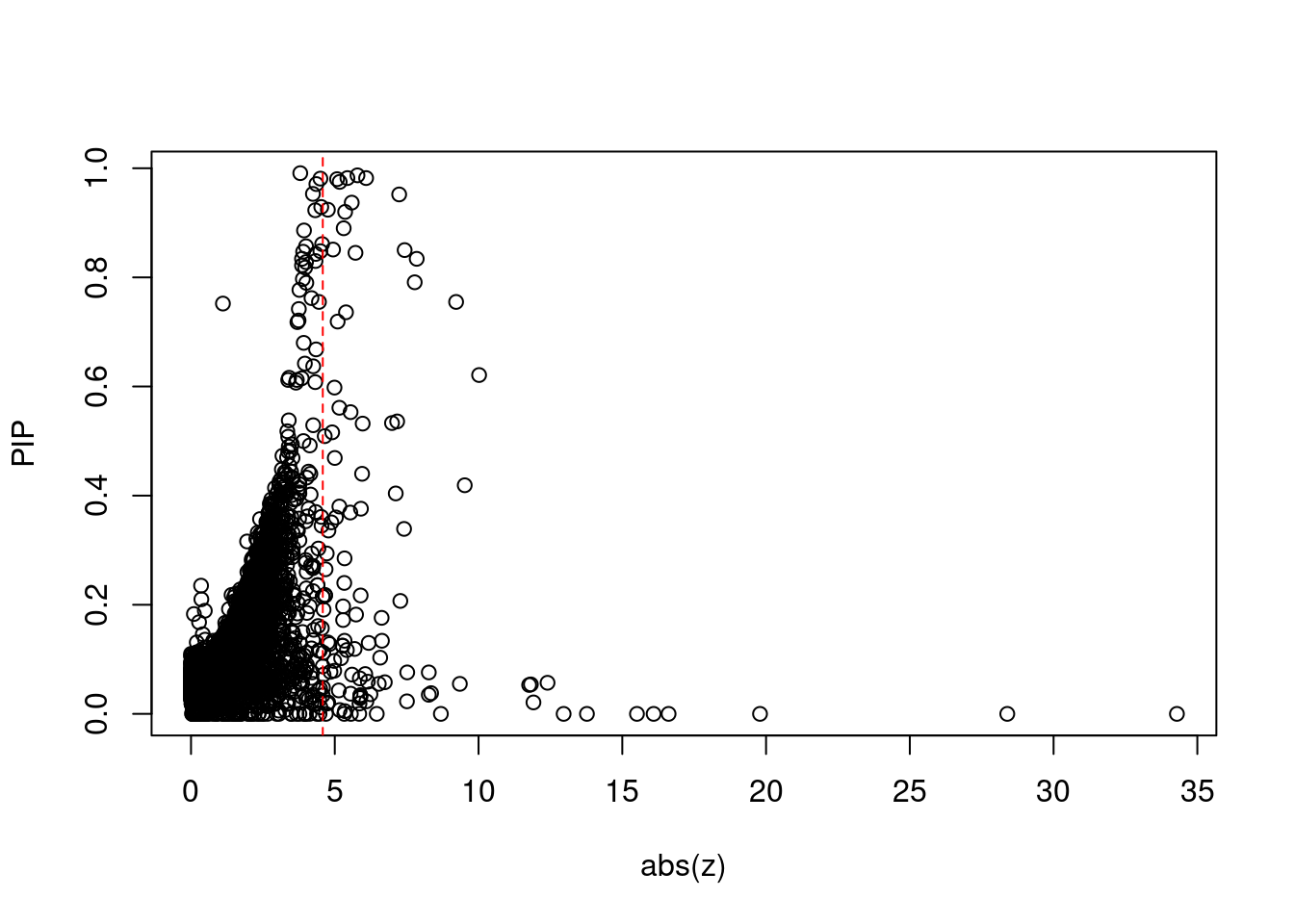
| Version | Author | Date |
|---|---|---|
| dfd2b5f | wesleycrouse | 2021-09-07 |
#proportion of significant z scores
mean(abs(ctwas_gene_res$z) > sig_thresh)
[1] 0.01027429#genes with most significant z scores
head(ctwas_gene_res[order(-abs(ctwas_gene_res$z)),report_cols],20) genename region_tag susie_pip mu2 PVE z
6880 TNFSF13 17_7 0.000 662.33 0.0e+00 34.29
3991 ATP1B2 17_7 0.000 509.63 1.1e-15 -28.39
6883 EIF4A1 17_7 0.000 428.99 0.0e+00 -19.79
11399 TNFSF12 17_7 0.000 288.75 0.0e+00 16.61
9477 DNAH2 17_7 0.000 193.10 0.0e+00 16.09
5311 WRAP53 17_7 0.000 204.81 8.2e-13 -15.51
5313 SAT2 17_7 0.000 208.24 1.5e-19 -13.77
6881 SENP3 17_7 0.000 283.01 2.8e-13 12.96
11526 GS1-259H13.2 7_61 0.057 128.99 2.4e-05 12.40
2887 NRBP1 2_16 0.021 80.67 5.5e-06 -11.91
2139 PTCD1 7_61 0.054 117.14 2.0e-05 11.82
6814 CPSF4 7_61 0.053 115.98 2.0e-05 11.76
8284 RBKS 2_16 0.621 68.48 1.4e-04 -10.02
10495 PRMT6 1_66 0.419 195.20 2.6e-04 -9.52
10415 ZNF789 7_61 0.055 74.23 1.3e-05 9.35
7355 BRI3 7_60 0.755 72.10 1.7e-04 -9.22
10851 UGT2B11 4_48 0.000 168.58 8.8e-08 -8.69
4936 SLC5A6 2_16 0.038 46.26 5.6e-06 -8.35
2611 MCM9 6_79 0.076 59.31 1.4e-05 8.27
4941 ATRAID 2_16 0.035 44.64 5.0e-06 8.27Locus plots for genes and SNPs
ctwas_gene_res_sortz <- ctwas_gene_res[order(-abs(ctwas_gene_res$z)),]

n_plots <- 5
for (region_tag_plot in head(unique(ctwas_gene_res_sortz$region_tag), n_plots)){
  ctwas_res_region <-  ctwas_res[ctwas_res$region_tag==region_tag_plot,]
  start <- min(ctwas_res_region$pos)
  end <- max(ctwas_res_region$pos)

  ctwas_res_region <- ctwas_res_region[order(ctwas_res_region$pos),]
  ctwas_res_region_gene <- ctwas_res_region[ctwas_res_region$type=="gene",]
  ctwas_res_region_snp <- ctwas_res_region[ctwas_res_region$type=="SNP",]

  #region name
  print(paste0("Region: ", region_tag_plot))

  #table of genes in region
  print(ctwas_res_region_gene[,report_cols])

  par(mfrow=c(4,1))

  #gene z scores
  plot(ctwas_res_region_gene$pos, abs(ctwas_res_region_gene$z), xlab="Position", ylab="abs(gene_z)", xlim=c(start,end),
   ylim=c(0,max(sig_thresh, abs(ctwas_res_region_gene$z))),
   main=paste0("Region: ", region_tag_plot))
  abline(h=sig_thresh,col="red",lty=2)

  #significance threshold for SNPs
  alpha_snp <- 5*10^(-8)
  sig_thresh_snp <- qnorm(1-alpha_snp/2, lower=T)

  #snp z scores
  plot(ctwas_res_region_snp$pos, abs(ctwas_res_region_snp$z), xlab="Position", ylab="abs(snp_z)",xlim=c(start,end),
   ylim=c(0,max(sig_thresh_snp, max(abs(ctwas_res_region_snp$z)))))
  abline(h=sig_thresh_snp,col="purple",lty=2)

  #gene pips
  plot(ctwas_res_region_gene$pos, ctwas_res_region_gene$susie_pip, xlab="Position", ylab="Gene PIP", xlim=c(start,end), ylim=c(0,1))
  abline(h=0.8,col="blue",lty=2)

  #snp pips
  plot(ctwas_res_region_snp$pos, ctwas_res_region_snp$susie_pip, xlab="Position", ylab="SNP PIP", xlim=c(start,end), ylim=c(0,1))
  abline(h=0.8,col="blue",lty=2)
}
[1] "Region: 17_7"
genename region_tag susie_pip mu2 PVE z
9229 TMEM102 17_7 0 21.43 0.0e+00 -6.46
6882 FGF11 17_7 0 13.19 0.0e+00 -1.61
11885 SLC35G6 17_7 0 159.03 0.0e+00 4.12
11399 TNFSF12 17_7 0 288.75 0.0e+00 16.61
6880 TNFSF13 17_7 0 662.33 0.0e+00 34.29
6881 SENP3 17_7 0 283.01 2.8e-13 12.96
6883 EIF4A1 17_7 0 428.99 0.0e+00 -19.79
5313 SAT2 17_7 0 208.24 1.5e-19 -13.77
3991 ATP1B2 17_7 0 509.63 1.1e-15 -28.39
5311 WRAP53 17_7 0 204.81 8.2e-13 -15.51
9477 DNAH2 17_7 0 193.10 0.0e+00 16.09
7853 TMEM88 17_7 0 22.07 0.0e+00 3.94
9115 AC025335.1 17_7 0 43.66 0.0e+00 4.38
8143 KCNAB3 17_7 0 31.03 0.0e+00 -2.11
8142 CNTROB 17_7 0 27.32 0.0e+00 -1.48
10982 VAMP2 17_7 0 28.65 0.0e+00 -2.11
9063 TMEM107 17_7 0 19.69 0.0e+00 -1.68
9059 AURKB 17_7 0 52.57 0.0e+00 -3.50
9053 CTC1 17_7 0 13.41 0.0e+00 1.64
9046 PFAS 17_7 0 7.07 0.0e+00 1.26
12191 RP11-849F2.9 17_7 0 8.66 0.0e+00 0.20
3703 SLC25A35 17_7 0 60.92 2.2e-20 3.48
9538 KRBA2 17_7 0 21.03 0.0e+00 -2.50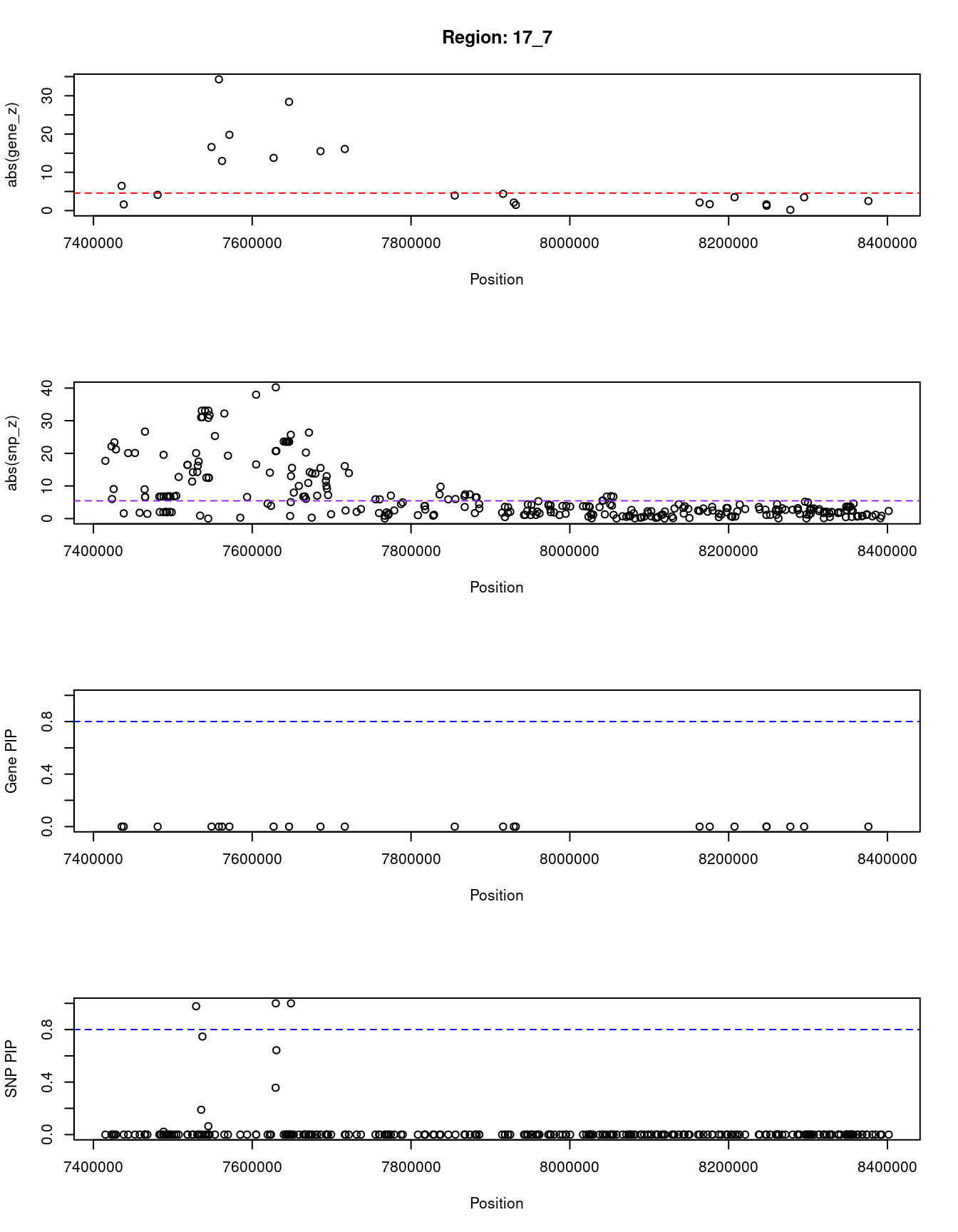
| Version | Author | Date |
|---|---|---|
| dfd2b5f | wesleycrouse | 2021-09-07 |
[1] "Region: 7_61"
             genename region_tag susie_pip    mu2     PVE     z
10451          SMURF1       7_61     0.210  15.02 1.0e-05  0.36
11449          ARPC1A       7_61     0.087  10.32 2.9e-06 -1.81
4077           ARPC1B       7_61     0.051   5.29 8.7e-07  1.12
2137            PDAP1       7_61     0.060  12.90 2.5e-06 -2.78
2138            BUD31       7_61     0.060  12.90 2.5e-06  2.78
6814            CPSF4       7_61     0.053 115.98 2.0e-05 11.76
11442          ATP5J2       7_61     0.100  11.81 3.8e-06 -2.00
2139            PTCD1       7_61     0.054 117.14 2.0e-05 11.82
10415          ZNF789       7_61     0.055  74.23 1.3e-05  9.35
10119         ZKSCAN5       7_61     0.058   5.85 1.1e-06  0.92
10222          ZNF655       7_61     0.156  13.70 6.8e-06  1.46
11526    GS1-259H13.2       7_61     0.057 128.99 2.4e-05 12.40
10175         ZSCAN25       7_61     0.060   6.53 1.3e-06  1.20
2140           CYP3A5       7_61     0.060   5.92 1.1e-06 -0.82
6809           CYP3A7       7_61     0.093   8.85 2.6e-06  0.25
12688 CYP3A7-CYP3A51P       7_61     0.093   8.85 2.6e-06  0.25
6808           CYP3A4       7_61     0.106  12.97 4.4e-06 -2.40
261           CYP3A43       7_61     0.090   9.85 2.9e-06 -1.66
5823            TRIM4       7_61     0.102  29.25 9.6e-06  5.22
2141          ZKSCAN1       7_61     0.053   7.82 1.3e-06  1.89
7633          ZSCAN21       7_61     0.057   8.68 1.6e-06 -2.22
7631             ZNF3       7_61     0.056   8.37 1.5e-06 -2.09
7628             MCM7       7_61     0.063   9.69 2.0e-06 -2.20
10986           AP4M1       7_61     0.074   7.47 1.8e-06 -0.88
7708            CNPY4       7_61     0.057   6.58 1.2e-06  1.16
2143             TAF6       7_61     0.051   9.82 1.6e-06 -2.62
10904          MBLAC1       7_61     0.106  11.78 4.0e-06  1.92
5820          C7orf43       7_61     0.063   9.59 1.9e-06  2.11
9884          LAMTOR4       7_61     0.092  10.34 3.0e-06 -1.74
3420            PILRB       7_61     0.054   6.52 1.1e-06  1.52
6803          PPP1R35       7_61     0.054   4.92 8.6e-07 -0.05
7696          TSC22D4       7_61     0.057   7.87 1.4e-06  1.89
7695            NYAP1       7_61     0.056   8.15 1.5e-06  2.04
2152            AGFG2       7_61     0.061   6.23 1.2e-06  1.03
10719           SAP25       7_61     0.064   6.48 1.3e-06  0.87
892             LRCH4       7_61     0.078   8.28 2.1e-06  1.14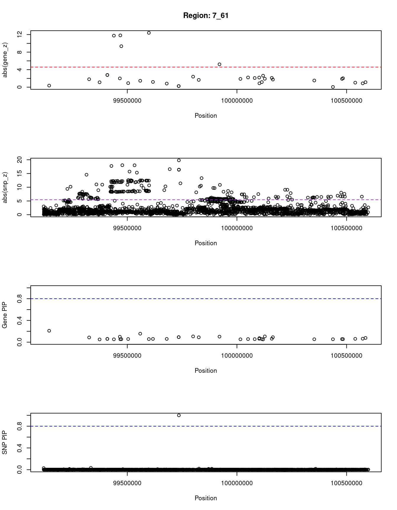
| Version | Author | Date |
|---|---|---|
| dfd2b5f | wesleycrouse | 2021-09-07 |
[1] "Region: 2_16"
      genename region_tag susie_pip   mu2     PVE      z
2881     CENPA       2_16     0.028  6.24 5.6e-07  -0.26
11149     OST4       2_16     0.021  5.12 3.4e-07  -0.98
4939   EMILIN1       2_16     0.021  7.94 5.4e-07   2.64
4927       KHK       2_16     0.034  7.72 8.5e-07   0.36
4935      PREB       2_16     0.033  9.35 1.0e-06  -2.03
4941    ATRAID       2_16     0.035 44.64 5.0e-06   8.27
4936    SLC5A6       2_16     0.038 46.26 5.6e-06  -8.35
1060       CAD       2_16     0.021 21.47 1.4e-06  -4.77
2885   SLC30A3       2_16     0.023 18.92 1.4e-06  -3.34
7169       UCN       2_16     0.055 26.46 4.7e-06  -6.53
2891     SNX17       2_16     0.023 47.48 3.5e-06   7.51
7170    ZNF513       2_16     0.022 15.38 1.1e-06  -3.61
2887     NRBP1       2_16     0.021 80.67 5.5e-06 -11.91
4925    IFT172       2_16     0.791 34.84 8.8e-05  -7.78
1058      GCKR       2_16     0.034 39.68 4.3e-06   5.89
10987  C2orf16       2_16     0.034 39.68 4.3e-06   5.89
10407     GPN1       2_16     0.029 29.61 2.8e-06  -5.88
8847   CCDC121       2_16     0.059 21.11 4.0e-06   3.78
6575       BRE       2_16     0.031 23.17 2.3e-06   5.89
8284      RBKS       2_16     0.621 68.48 1.4e-04 -10.02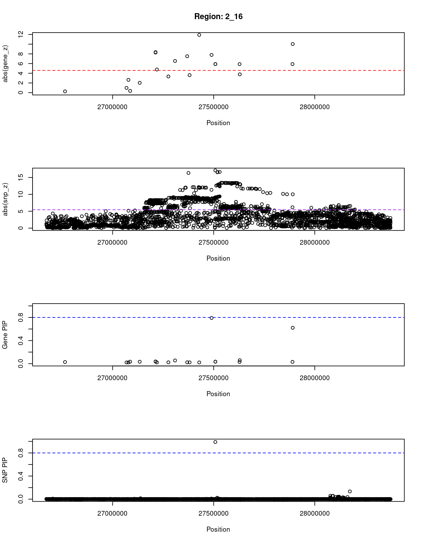
| Version | Author | Date |
|---|---|---|
| dfd2b5f | wesleycrouse | 2021-09-07 |
[1] "Region: 1_66"
      genename region_tag susie_pip   mu2     PVE     z
10495    PRMT6       1_66     0.419 195.2 0.00026 -9.52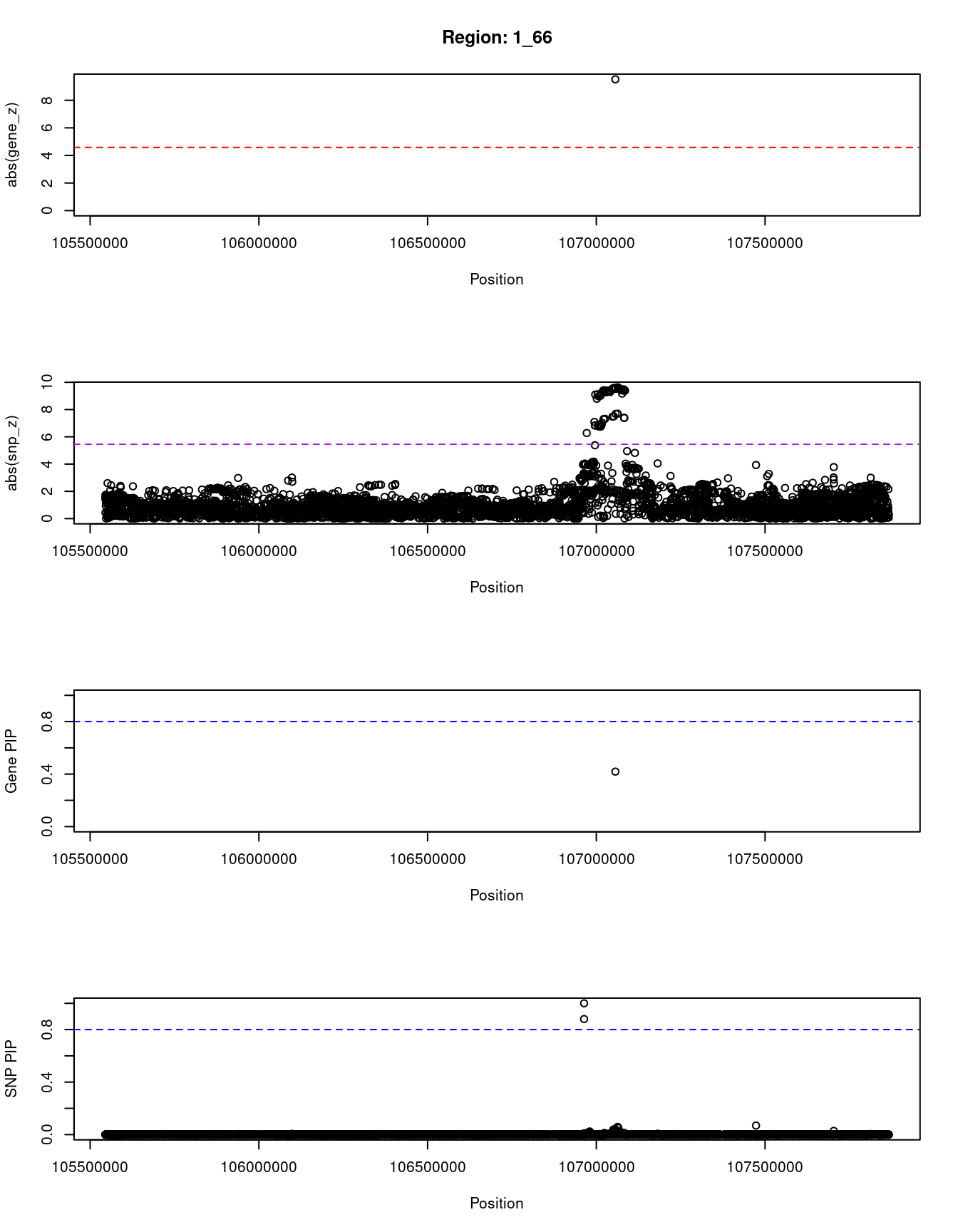
| Version | Author | Date |
|---|---|---|
| dfd2b5f | wesleycrouse | 2021-09-07 |
[1] "Region: 7_60"
     genename region_tag susie_pip   mu2     PVE     z
79       TAC1       7_60     0.048  5.44 8.4e-07  0.11
725      ASNS       7_60     0.047  5.79 8.7e-07  0.99
7356    LMTK2       7_60     0.059  6.78 1.3e-06 -0.34
9166  BHLHA15       7_60     0.048  5.54 8.6e-07 -0.54
7355     BRI3       7_60     0.755 72.10 1.7e-04 -9.22
86   BAIAP2L1       7_60     0.079 27.52 7.0e-06 -4.98
2136    NPTX2       7_60     0.064  7.80 1.6e-06 -0.89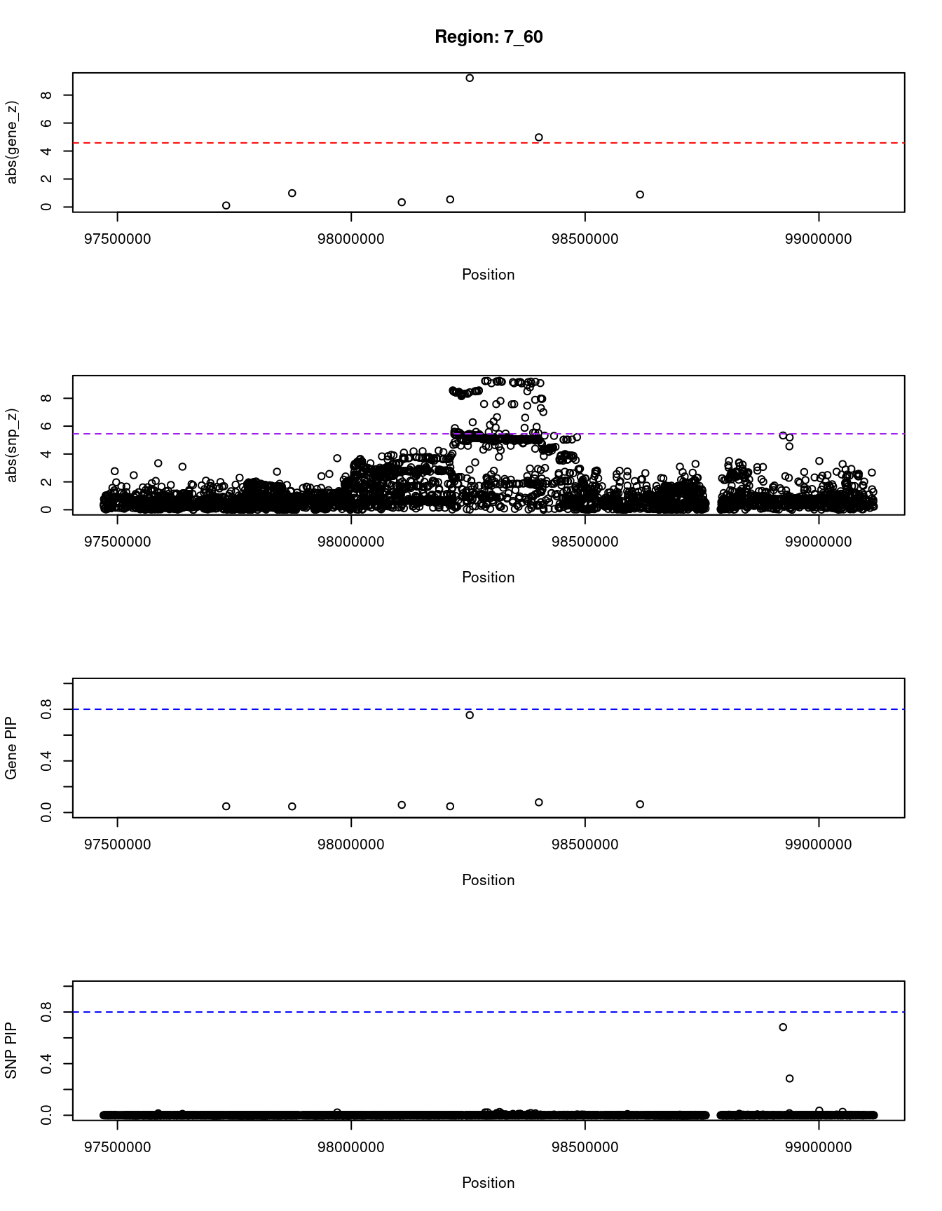
| Version | Author | Date |
|---|---|---|
| dfd2b5f | wesleycrouse | 2021-09-07 |
SNPs with highest PIPs
#snps with PIP>0.8 or 20 highest PIPs
head(ctwas_snp_res[order(-ctwas_snp_res$susie_pip),report_cols_snps],
max(sum(ctwas_snp_res$susie_pip>0.8), 20))
id region_tag susie_pip mu2 PVE z
28001 rs12029116 1_62 1.000 111.92 3.6e-04 10.77
74194 rs11124265 2_20 1.000 71.08 2.3e-04 11.99
74468 rs72787520 2_20 1.000 97.02 3.1e-04 13.91
74687 rs112564689 2_21 1.000 35.86 1.1e-04 5.91
164560 rs768688512 3_58 1.000 547.62 1.8e-03 3.17
197497 rs5855544 3_120 1.000 50.14 1.6e-04 -7.28
359670 rs199804242 6_89 1.000 5938.24 1.9e-02 -2.78
507924 rs17134158 10_6 1.000 54.86 1.8e-04 -9.64
571434 rs754042 11_41 1.000 37.93 1.2e-04 -5.56
737765 rs9931108 16_45 1.000 91.30 2.9e-04 7.38
737794 rs57960111 16_45 1.000 171.02 5.5e-04 1.51
744788 rs62059839 17_7 1.000 1119.62 3.6e-03 40.23
744799 rs72829446 17_7 1.000 234.93 7.5e-04 13.01
785689 rs141207866 18_43 1.000 55.15 1.8e-04 7.59
791922 rs8111359 19_9 1.000 44.89 1.4e-04 -6.68
866680 rs147660689 1_66 1.000 1139.88 3.7e-03 -1.71
885074 rs201939100 4_48 1.000 781.15 2.5e-03 -3.70
952291 rs45446698 7_61 1.000 351.97 1.1e-03 -19.79
1046009 rs61371437 19_34 1.000 12937.27 4.1e-02 4.54
1046018 rs113176985 19_34 1.000 12946.01 4.1e-02 4.53
1046021 rs374141296 19_34 1.000 12940.89 4.1e-02 3.70
7810 rs79598313 1_18 0.999 44.87 1.4e-04 -6.64
592561 rs12319562 12_3 0.999 39.66 1.3e-04 5.23
744713 rs62059238 17_6 0.998 51.79 1.7e-04 7.31
744723 rs73233955 17_6 0.997 50.28 1.6e-04 -6.19
448706 rs4236857 8_56 0.996 30.18 9.6e-05 5.27
54059 rs17558745 1_110 0.995 29.84 9.5e-05 -5.32
199284 rs36205397 4_4 0.995 56.52 1.8e-04 7.71
723632 rs2764772 16_18 0.994 36.27 1.2e-04 6.15
737791 rs12934751 16_45 0.992 86.44 2.7e-04 -8.48
1033389 rs146497684 19_14 0.992 91.35 2.9e-04 9.93
231314 rs116652741 4_68 0.990 30.37 9.6e-05 -4.88
875747 rs1260326 2_16 0.990 219.36 7.0e-04 17.10
525722 rs11510917 10_39 0.983 39.70 1.3e-04 -6.25
74265 rs10439444 2_20 0.980 37.92 1.2e-04 -6.99
476565 rs12683780 9_13 0.979 27.39 8.6e-05 -4.99
73036 rs7606480 2_17 0.978 28.14 8.8e-05 5.06
412239 rs125124 7_80 0.978 26.71 8.4e-05 4.89
744761 rs142700974 17_7 0.978 155.36 4.9e-04 -20.08
483145 rs11557154 9_26 0.977 27.69 8.7e-05 4.77
673973 rs72681869 14_20 0.970 26.97 8.4e-05 4.99
41812 rs10798655 1_89 0.968 60.23 1.9e-04 -8.15
449852 rs382796 8_57 0.968 28.67 8.9e-05 5.35
570379 rs72932198 11_38 0.965 27.12 8.4e-05 -5.27
52605 rs3754140 1_108 0.964 26.99 8.3e-05 4.53
52648 rs1223802 1_108 0.963 31.24 9.6e-05 -5.11
301220 rs329123 5_80 0.951 28.42 8.7e-05 -5.03
1022562 rs17637241 17_28 0.950 51.53 1.6e-04 7.79
14507 rs12751490 1_35 0.947 26.76 8.1e-05 4.93
570416 rs12804411 11_38 0.939 28.28 8.5e-05 5.35
691989 rs34639393 14_56 0.930 32.12 9.6e-05 -5.50
622720 rs375115050 12_59 0.929 26.02 7.7e-05 -4.88
73641 rs76886327 2_18 0.925 25.75 7.6e-05 -4.73
283069 rs2928169 5_45 0.921 26.47 7.8e-05 4.44
350526 rs4515420 6_70 0.919 45.06 1.3e-04 6.30
97094 rs590097 2_66 0.909 51.29 1.5e-04 7.41
33737 rs10788826 1_74 0.905 26.50 7.7e-05 4.83
477772 rs112107457 9_15 0.893 39.17 1.1e-04 5.99
49532 rs4951319 1_103 0.892 39.91 1.1e-04 6.26
498503 rs201250488 9_56 0.888 31.86 9.1e-05 -5.36
866681 rs77477013 1_66 0.880 1137.83 3.2e-03 -1.86
626095 rs75622376 12_67 0.878 25.30 7.1e-05 4.67
359785 rs62431291 6_90 0.874 25.66 7.2e-05 -4.61
818377 rs3212201 20_28 0.869 41.05 1.1e-04 6.39
555237 rs11024433 11_13 0.861 26.90 7.4e-05 -4.89
403640 rs34048349 7_62 0.854 24.38 6.7e-05 -3.40
545343 rs2225079 10_78 0.852 25.56 7.0e-05 4.56
499036 rs3904316 9_58 0.849 24.64 6.7e-05 -4.34
377257 rs117483607 7_14 0.848 26.04 7.1e-05 -4.66
438996 rs12543287 8_37 0.847 25.66 7.0e-05 4.29
157712 rs73128974 3_44 0.844 28.43 7.7e-05 5.06
689846 rs35604463 14_52 0.831 26.32 7.0e-05 4.65
16190 rs137898851 1_39 0.829 26.04 6.9e-05 4.60
453088 rs369077882 8_64 0.824 25.54 6.7e-05 -4.48
571427 rs341048 11_41 0.823 25.48 6.7e-05 -3.79SNPs with largest effect sizes
#plot PIP vs effect size
plot(ctwas_snp_res$susie_pip, ctwas_snp_res$mu2, xlab="PIP", ylab="mu^2", main="SNP PIPs vs Effect Size")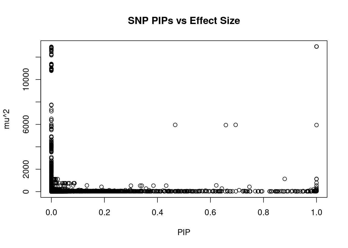
| Version | Author | Date |
|---|---|---|
| dfd2b5f | wesleycrouse | 2021-09-07 |
#SNPs with 50 largest effect sizes
head(ctwas_snp_res[order(-ctwas_snp_res$mu2),report_cols_snps],50)
id region_tag susie_pip mu2 PVE z
1046018 rs113176985 19_34 1 12946.01 4.1e-02 4.53
1046021 rs374141296 19_34 1 12940.89 4.1e-02 3.70
1046009 rs61371437 19_34 1 12937.27 4.1e-02 4.54
1046011 rs35295508 19_34 0 12917.38 7.7e-08 4.62
1045999 rs739349 19_34 0 12884.35 4.4e-07 4.50
1046000 rs756628 19_34 0 12884.23 3.7e-07 4.49
1046025 rs2946865 19_34 0 12874.38 6.3e-12 4.49
1046016 rs73056069 19_34 0 12867.69 1.9e-11 4.53
1045996 rs739347 19_34 0 12863.07 7.3e-08 4.56
1045997 rs2073614 19_34 0 12849.79 4.9e-10 4.55
1046013 rs2878354 19_34 0 12842.16 1.7e-13 4.59
1046002 rs2077300 19_34 0 12809.80 2.0e-14 4.45
1045992 rs4802613 19_34 0 12788.97 9.1e-18 4.43
1046006 rs73056059 19_34 0 12787.54 9.0e-15 4.50
1046026 rs60815603 19_34 0 12693.76 0.0e+00 4.58
1046029 rs1316885 19_34 0 12628.47 0.0e+00 4.45
1045990 rs10403394 19_34 0 12621.40 0.0e+00 4.69
1045991 rs17555056 19_34 0 12616.20 0.0e+00 4.67
1046031 rs60746284 19_34 0 12610.93 0.0e+00 4.52
1046034 rs2946863 19_34 0 12606.33 0.0e+00 4.49
1046027 rs35443645 19_34 0 12596.67 0.0e+00 4.51
1046007 rs73056062 19_34 0 12456.99 0.0e+00 4.40
1046037 rs553431297 19_34 0 12277.21 0.0e+00 4.65
1046020 rs112283514 19_34 0 12226.63 0.0e+00 4.24
1046022 rs11270139 19_34 0 12166.28 0.0e+00 4.80
1045987 rs10421294 19_34 0 11386.36 0.0e+00 4.01
1045986 rs8108175 19_34 0 11384.71 0.0e+00 4.01
1045979 rs59192944 19_34 0 11362.90 0.0e+00 4.00
1045985 rs1858742 19_34 0 11362.86 0.0e+00 3.98
1045976 rs55991145 19_34 0 11354.75 0.0e+00 3.99
1045971 rs3786567 19_34 0 11350.20 0.0e+00 3.98
1045967 rs2271952 19_34 0 11345.86 0.0e+00 3.98
1045970 rs4801801 19_34 0 11345.58 0.0e+00 3.97
1045966 rs2271953 19_34 0 11333.45 0.0e+00 3.98
1045968 rs2271951 19_34 0 11333.42 0.0e+00 3.99
1045957 rs60365978 19_34 0 11321.25 0.0e+00 3.94
1045963 rs4802612 19_34 0 11275.26 0.0e+00 3.94
1045973 rs2517977 19_34 0 11258.67 0.0e+00 3.95
1045960 rs55893003 19_34 0 11242.74 0.0e+00 3.97
1045952 rs55992104 19_34 0 10979.94 0.0e+00 3.84
1045946 rs60403475 19_34 0 10976.93 0.0e+00 3.84
1045949 rs4352151 19_34 0 10976.13 0.0e+00 3.82
1045943 rs11878448 19_34 0 10968.32 0.0e+00 3.81
1045937 rs9653100 19_34 0 10965.13 0.0e+00 3.84
1045933 rs4802611 19_34 0 10956.86 0.0e+00 3.80
1045925 rs7251338 19_34 0 10939.95 0.0e+00 3.79
1045924 rs59269605 19_34 0 10939.19 0.0e+00 3.80
1045945 rs1042120 19_34 0 10910.70 0.0e+00 3.80
1045941 rs113220577 19_34 0 10901.28 0.0e+00 3.80
1045935 rs9653118 19_34 0 10885.30 0.0e+00 3.83SNPs with highest PVE
#SNPs with 50 highest pve
head(ctwas_snp_res[order(-ctwas_snp_res$PVE),report_cols_snps],50)
id region_tag susie_pip mu2 PVE z
1046009 rs61371437 19_34 1.000 12937.27 0.04100 4.54
1046018 rs113176985 19_34 1.000 12946.01 0.04100 4.53
1046021 rs374141296 19_34 1.000 12940.89 0.04100 3.70
359670 rs199804242 6_89 1.000 5938.24 0.01900 -2.78
359669 rs2327654 6_89 0.695 5954.40 0.01300 -2.39
359673 rs113527452 6_89 0.658 5936.22 0.01300 -2.51
359686 rs6923513 6_89 0.467 5954.01 0.00890 -2.38
866680 rs147660689 1_66 1.000 1139.88 0.00370 -1.71
744788 rs62059839 17_7 1.000 1119.62 0.00360 40.23
866681 rs77477013 1_66 0.880 1137.83 0.00320 -1.86
885074 rs201939100 4_48 1.000 781.15 0.00250 -3.70
164560 rs768688512 3_58 1.000 547.62 0.00180 3.17
526910 rs1935 10_42 0.622 558.81 0.00110 27.16
952291 rs45446698 7_61 1.000 351.97 0.00110 -19.79
744768 rs8073177 17_7 0.747 432.53 0.00100 31.09
744799 rs72829446 17_7 1.000 234.93 0.00075 13.01
164557 rs12493756 3_58 0.433 535.61 0.00074 3.02
875747 rs1260326 2_16 0.990 219.36 0.00070 17.10
164558 rs12493835 3_58 0.385 535.83 0.00066 3.00
164555 rs138503435 3_58 0.341 535.50 0.00059 3.00
164559 rs6765538 3_58 0.335 535.61 0.00058 2.96
744789 rs6257 17_7 0.643 274.77 0.00057 -20.73
737794 rs57960111 16_45 1.000 171.02 0.00055 1.51
164556 rs73141241 3_58 0.300 533.00 0.00051 3.01
744761 rs142700974 17_7 0.978 155.36 0.00049 -20.08
28001 rs12029116 1_62 1.000 111.92 0.00036 10.77
74468 rs72787520 2_20 1.000 97.02 0.00031 13.91
744787 rs112885647 17_7 0.357 273.13 0.00031 -20.68
1001733 rs56332871 15_46 0.708 132.93 0.00030 11.61
737765 rs9931108 16_45 1.000 91.30 0.00029 7.38
1033389 rs146497684 19_14 0.992 91.35 0.00029 9.93
737791 rs12934751 16_45 0.992 86.44 0.00027 -8.48
744766 rs9892862 17_7 0.189 428.72 0.00026 31.04
526921 rs10761729 10_42 0.134 555.06 0.00024 27.10
74194 rs11124265 2_20 1.000 71.08 0.00023 11.99
885080 rs11932983 4_48 0.086 754.04 0.00021 -2.36
885103 rs60276248 4_48 0.087 753.56 0.00021 -2.38
885106 rs56943005 4_48 0.087 753.55 0.00021 -2.38
885075 rs2125307 4_48 0.084 754.00 0.00020 -2.36
41812 rs10798655 1_89 0.968 60.23 0.00019 -8.15
199284 rs36205397 4_4 0.995 56.52 0.00018 7.71
507924 rs17134158 10_6 1.000 54.86 0.00018 -9.64
785689 rs141207866 18_43 1.000 55.15 0.00018 7.59
634076 rs606950 13_3 0.581 92.04 0.00017 9.88
744713 rs62059238 17_6 0.998 51.79 0.00017 7.31
164581 rs9310061 3_58 0.298 162.56 0.00016 -5.57
197497 rs5855544 3_120 1.000 50.14 0.00016 -7.28
737802 rs6564897 16_45 0.368 132.90 0.00016 4.61
744723 rs73233955 17_6 0.997 50.28 0.00016 -6.19
885128 rs55831171 4_48 0.068 753.32 0.00016 -2.37SNPs with largest z scores
#SNPs with 50 largest z scores
head(ctwas_snp_res[order(-abs(ctwas_snp_res$z)),report_cols_snps],50)
id region_tag susie_pip mu2 PVE z
744788 rs62059839 17_7 1.000 1119.62 3.6e-03 40.23
744782 rs149932962 17_7 0.000 920.97 0.0e+00 37.98
744769 rs62059797 17_7 0.000 674.05 0.0e+00 33.12
744767 rs35049113 17_7 0.000 670.55 0.0e+00 33.07
744773 rs12941509 17_7 0.000 677.90 0.0e+00 33.07
744778 rs4968212 17_7 0.000 657.28 0.0e+00 -32.21
744776 rs62059801 17_7 0.000 628.74 0.0e+00 31.72
744768 rs8073177 17_7 0.747 432.53 1.0e-03 31.09
744766 rs9892862 17_7 0.189 428.72 2.6e-04 31.04
744772 rs11078694 17_7 0.064 429.44 8.8e-05 -30.85
526910 rs1935 10_42 0.622 558.81 1.1e-03 27.16
526921 rs10761729 10_42 0.134 555.06 2.4e-04 27.10
526941 rs5785566 10_42 0.082 554.11 1.5e-04 27.08
526957 rs6479896 10_42 0.050 553.13 8.9e-05 27.06
526953 rs10822160 10_42 0.045 552.36 7.9e-05 27.05
526959 rs7910927 10_42 0.035 552.32 6.3e-05 27.05
526974 rs3956912 10_42 0.017 550.26 2.9e-05 27.02
526965 rs10822168 10_42 0.012 549.44 2.1e-05 27.00
526905 rs35751397 10_42 0.005 547.22 8.3e-06 26.94
526967 rs10640079 10_42 0.001 545.15 1.8e-06 26.85
744737 rs34474914 17_7 0.000 430.02 0.0e+00 26.65
744808 rs1641549 17_7 0.000 269.62 1.9e-19 -26.37
744798 rs745412832 17_7 0.000 314.54 7.8e-19 25.69
527002 rs2163188 10_42 0.000 482.00 6.9e-07 -25.42
526943 rs10761739 10_42 0.005 518.18 8.1e-06 25.34
744777 rs12601581 17_7 0.000 452.55 0.0e+00 -25.31
527010 rs10822186 10_42 0.000 473.88 1.9e-07 25.11
527011 rs7895549 10_42 0.000 473.45 1.9e-07 25.09
527009 rs570234162 10_42 0.000 469.42 1.8e-07 -24.96
527006 rs4746205 10_42 0.000 468.96 6.6e-07 -24.92
527007 rs7090758 10_42 0.000 447.03 3.6e-07 -24.39
744790 rs1642797 17_7 0.000 448.12 1.3e-18 23.61
744791 rs1642808 17_7 0.000 447.00 1.1e-18 23.57
744792 rs1641538 17_7 0.000 447.02 1.1e-18 23.57
744793 rs1641531 17_7 0.000 446.68 1.1e-18 23.57
744794 rs1641528 17_7 0.000 447.28 1.3e-18 23.57
744795 rs1641522 17_7 0.000 447.10 1.3e-18 23.55
526895 rs10995445 10_42 0.000 404.11 2.2e-07 23.42
744730 rs13290 17_7 0.000 133.37 0.0e+00 23.39
744727 rs11652328 17_7 0.000 311.97 0.0e+00 22.13
744731 rs34706172 17_7 0.000 132.63 0.0e+00 21.20
744789 rs6257 17_7 0.643 274.77 5.7e-04 -20.73
744787 rs112885647 17_7 0.357 273.13 3.1e-04 -20.68
744805 rs4968186 17_7 0.000 189.60 0.0e+00 20.23
744734 rs12600863 17_7 0.000 154.17 0.0e+00 20.11
744733 rs3829603 17_7 0.000 156.46 0.0e+00 20.08
744761 rs142700974 17_7 0.978 155.36 4.9e-04 -20.08
952291 rs45446698 7_61 1.000 351.97 1.1e-03 -19.79
744746 rs116560331 17_7 0.022 146.07 1.0e-05 -19.55
744779 rs12939472 17_7 0.000 242.67 0.0e+00 -19.28Gene set enrichment for genes with PIP>0.8
#GO enrichment analysis
library(enrichR)
Welcome to enrichR
Checking connection ... Enrichr ... Connection is Live!
FlyEnrichr ... Connection is available!
WormEnrichr ... Connection is available!
YeastEnrichr ... Connection is available!
FishEnrichr ... Connection is available!dbs <- c("GO_Biological_Process_2021", "GO_Cellular_Component_2021", "GO_Molecular_Function_2021")
genes <- ctwas_gene_res$genename[ctwas_gene_res$susie_pip>0.8]
#number of genes for gene set enrichment
length(genes)[1] 31if (length(genes)>0){
GO_enrichment <- enrichr(genes, dbs)
for (db in dbs){
print(db)
df <- GO_enrichment[[db]]
df <- df[df$Adjusted.P.value<0.05,c("Term", "Overlap", "Adjusted.P.value", "Genes")]
print(df)
}
#DisGeNET enrichment
# devtools::install_bitbucket("ibi_group/disgenet2r")
library(disgenet2r)
disgenet_api_key <- get_disgenet_api_key(
email = "wesleycrouse@gmail.com",
password = "uchicago1" )
Sys.setenv(DISGENET_API_KEY= disgenet_api_key)
res_enrich <-disease_enrichment(entities=genes, vocabulary = "HGNC",
database = "CURATED" )
df <- res_enrich@qresult[1:10, c("Description", "FDR", "Ratio", "BgRatio")]
print(df)
#WebGestalt enrichment
library(WebGestaltR)
background <- ctwas_gene_res$genename
#listGeneSet()
databases <- c("pathway_KEGG", "disease_GLAD4U", "disease_OMIM")
enrichResult <- WebGestaltR(enrichMethod="ORA", organism="hsapiens",
interestGene=genes, referenceGene=background,
enrichDatabase=databases, interestGeneType="genesymbol",
referenceGeneType="genesymbol", isOutput=F)
print(enrichResult[,c("description", "size", "overlap", "FDR", "database", "userId")])
}Uploading data to Enrichr... Done.
Querying GO_Biological_Process_2021... Done.
Querying GO_Cellular_Component_2021... Done.
Querying GO_Molecular_Function_2021... Done.
Parsing results... Done.
[1] "GO_Biological_Process_2021"
[1] Term Overlap Adjusted.P.value Genes
<0 rows> (or 0-length row.names)
[1] "GO_Cellular_Component_2021"
[1] Term Overlap Adjusted.P.value Genes
<0 rows> (or 0-length row.names)
[1] "GO_Molecular_Function_2021"
[1] Term Overlap Adjusted.P.value Genes
<0 rows> (or 0-length row.names)ZNF219 gene(s) from the input list not found in DisGeNET CURATEDLINC01612 gene(s) from the input list not found in DisGeNET CURATEDMIEF1 gene(s) from the input list not found in DisGeNET CURATEDAC098828.2 gene(s) from the input list not found in DisGeNET CURATEDRMI1 gene(s) from the input list not found in DisGeNET CURATEDNTAN1 gene(s) from the input list not found in DisGeNET CURATEDURB1-AS1 gene(s) from the input list not found in DisGeNET CURATEDMLXIP gene(s) from the input list not found in DisGeNET CURATEDRP3-413H6.2 gene(s) from the input list not found in DisGeNET CURATEDAKNA gene(s) from the input list not found in DisGeNET CURATEDDLEU1 gene(s) from the input list not found in DisGeNET CURATEDRP11-327J17.2 gene(s) from the input list not found in DisGeNET CURATEDLINC00672 gene(s) from the input list not found in DisGeNET CURATEDPTTG1IP gene(s) from the input list not found in DisGeNET CURATED Description
51 Neoplasms, Glandular and Epithelial
81 Glandular Neoplasms
94 Deficiency of prolidase
100 Acute Undifferentiated Leukemia
107 Wrinkly skin syndrome
120 Undifferentiated type acute leukemia
127 Acute myeloid leukemia, 11q23 abnormalities
129 Epithelioma
135 SPLIT-HAND/FOOT MALFORMATION 3
136 Growth Deficiency and Mental Retardation with Facial Dysmorphism
FDR Ratio BgRatio
51 0.03851696 1/17 2/9703
81 0.03851696 1/17 2/9703
94 0.03851696 1/17 1/9703
100 0.03851696 1/17 1/9703
107 0.03851696 1/17 2/9703
120 0.03851696 1/17 1/9703
127 0.03851696 1/17 1/9703
129 0.03851696 1/17 2/9703
135 0.03851696 1/17 1/9703
136 0.03851696 1/17 2/9703******************************************
* *
* Welcome to WebGestaltR ! *
* *
******************************************Loading the functional categories...
Loading the ID list...
Loading the reference list...
Performing the enrichment analysis...Warning in oraEnrichment(interestGeneList, referenceGeneList, geneSet,
minNum = minNum, : No significant gene set is identified based on FDR 0.05!NULL
sessionInfo()R version 3.6.1 (2019-07-05)
Platform: x86_64-pc-linux-gnu (64-bit)
Running under: Scientific Linux 7.4 (Nitrogen)
Matrix products: default
BLAS/LAPACK: /software/openblas-0.2.19-el7-x86_64/lib/libopenblas_haswellp-r0.2.19.so
locale:
[1] LC_CTYPE=en_US.UTF-8 LC_NUMERIC=C
[3] LC_TIME=en_US.UTF-8 LC_COLLATE=en_US.UTF-8
[5] LC_MONETARY=en_US.UTF-8 LC_MESSAGES=en_US.UTF-8
[7] LC_PAPER=en_US.UTF-8 LC_NAME=C
[9] LC_ADDRESS=C LC_TELEPHONE=C
[11] LC_MEASUREMENT=en_US.UTF-8 LC_IDENTIFICATION=C
attached base packages:
[1] stats graphics grDevices utils datasets methods base
other attached packages:
[1] WebGestaltR_0.4.4 disgenet2r_0.99.2 enrichR_3.0 cowplot_1.0.0
[5] ggplot2_3.3.3
loaded via a namespace (and not attached):
[1] bitops_1.0-6 matrixStats_0.57.0
[3] fs_1.3.1 bit64_4.0.5
[5] doParallel_1.0.16 progress_1.2.2
[7] httr_1.4.1 rprojroot_2.0.2
[9] GenomeInfoDb_1.20.0 doRNG_1.8.2
[11] tools_3.6.1 utf8_1.2.1
[13] R6_2.5.0 DBI_1.1.1
[15] BiocGenerics_0.30.0 colorspace_1.4-1
[17] withr_2.4.1 tidyselect_1.1.0
[19] prettyunits_1.0.2 bit_4.0.4
[21] curl_3.3 compiler_3.6.1
[23] git2r_0.26.1 Biobase_2.44.0
[25] DelayedArray_0.10.0 rtracklayer_1.44.0
[27] labeling_0.3 scales_1.1.0
[29] readr_1.4.0 apcluster_1.4.8
[31] stringr_1.4.0 digest_0.6.20
[33] Rsamtools_2.0.0 svglite_1.2.2
[35] rmarkdown_1.13 XVector_0.24.0
[37] pkgconfig_2.0.3 htmltools_0.3.6
[39] fastmap_1.1.0 BSgenome_1.52.0
[41] rlang_0.4.11 RSQLite_2.2.7
[43] generics_0.0.2 farver_2.1.0
[45] jsonlite_1.6 BiocParallel_1.18.0
[47] dplyr_1.0.7 VariantAnnotation_1.30.1
[49] RCurl_1.98-1.1 magrittr_2.0.1
[51] GenomeInfoDbData_1.2.1 Matrix_1.2-18
[53] Rcpp_1.0.6 munsell_0.5.0
[55] S4Vectors_0.22.1 fansi_0.5.0
[57] gdtools_0.1.9 lifecycle_1.0.0
[59] stringi_1.4.3 whisker_0.3-2
[61] yaml_2.2.0 SummarizedExperiment_1.14.1
[63] zlibbioc_1.30.0 plyr_1.8.4
[65] grid_3.6.1 blob_1.2.1
[67] parallel_3.6.1 promises_1.0.1
[69] crayon_1.4.1 lattice_0.20-38
[71] Biostrings_2.52.0 GenomicFeatures_1.36.3
[73] hms_1.1.0 knitr_1.23
[75] pillar_1.6.1 igraph_1.2.4.1
[77] GenomicRanges_1.36.0 rjson_0.2.20
[79] rngtools_1.5 codetools_0.2-16
[81] reshape2_1.4.3 biomaRt_2.40.1
[83] stats4_3.6.1 XML_3.98-1.20
[85] glue_1.4.2 evaluate_0.14
[87] data.table_1.14.0 foreach_1.5.1
[89] vctrs_0.3.8 httpuv_1.5.1
[91] gtable_0.3.0 purrr_0.3.4
[93] assertthat_0.2.1 cachem_1.0.5
[95] xfun_0.8 later_0.8.0
[97] tibble_3.1.2 iterators_1.0.13
[99] GenomicAlignments_1.20.1 AnnotationDbi_1.46.0
[101] memoise_2.0.0 IRanges_2.18.1
[103] workflowr_1.6.2 ellipsis_0.3.2