Total bilirubin (quantile) - Liver
wesleycrouse
2021-09-09
Last updated: 2021-09-09
Checks: 6 1
Knit directory: ctwas_applied/
This reproducible R Markdown analysis was created with workflowr (version 1.6.2). The Checks tab describes the reproducibility checks that were applied when the results were created. The Past versions tab lists the development history.
The R Markdown file has unstaged changes. To know which version of the R Markdown file created these results, you’ll want to first commit it to the Git repo. If you’re still working on the analysis, you can ignore this warning. When you’re finished, you can run wflow_publish to commit the R Markdown file and build the HTML.
Great job! The global environment was empty. Objects defined in the global environment can affect the analysis in your R Markdown file in unknown ways. For reproduciblity it’s best to always run the code in an empty environment.
The command set.seed(20210726) was run prior to running the code in the R Markdown file. Setting a seed ensures that any results that rely on randomness, e.g. subsampling or permutations, are reproducible.
Great job! Recording the operating system, R version, and package versions is critical for reproducibility.
Nice! There were no cached chunks for this analysis, so you can be confident that you successfully produced the results during this run.
Great job! Using relative paths to the files within your workflowr project makes it easier to run your code on other machines.
Great! You are using Git for version control. Tracking code development and connecting the code version to the results is critical for reproducibility.
The results in this page were generated with repository version 59e5f4d. See the Past versions tab to see a history of the changes made to the R Markdown and HTML files.
Note that you need to be careful to ensure that all relevant files for the analysis have been committed to Git prior to generating the results (you can use wflow_publish or wflow_git_commit). workflowr only checks the R Markdown file, but you know if there are other scripts or data files that it depends on. Below is the status of the Git repository when the results were generated:
Unstaged changes:
    Modified:   analysis/ukb-d-30500_irnt_Liver.Rmd
    Modified:   analysis/ukb-d-30600_irnt_Liver.Rmd
    Modified:   analysis/ukb-d-30610_irnt_Liver.Rmd
    Modified:   analysis/ukb-d-30620_irnt_Liver.Rmd
    Modified:   analysis/ukb-d-30630_irnt_Liver.Rmd
    Modified:   analysis/ukb-d-30640_irnt_Liver.Rmd
    Modified:   analysis/ukb-d-30650_irnt_Liver.Rmd
    Modified:   analysis/ukb-d-30660_irnt_Liver.Rmd
    Modified:   analysis/ukb-d-30670_irnt_Liver.Rmd
    Modified:   analysis/ukb-d-30680_irnt_Liver.Rmd
    Modified:   analysis/ukb-d-30690_irnt_Liver.Rmd
    Modified:   analysis/ukb-d-30700_irnt_Liver.Rmd
    Modified:   analysis/ukb-d-30710_irnt_Liver.Rmd
    Modified:   analysis/ukb-d-30720_irnt_Liver.Rmd
    Modified:   analysis/ukb-d-30730_irnt_Liver.Rmd
    Modified:   analysis/ukb-d-30740_irnt_Liver.Rmd
    Modified:   analysis/ukb-d-30750_irnt_Liver.Rmd
    Modified:   analysis/ukb-d-30760_irnt_Liver.Rmd
    Modified:   analysis/ukb-d-30770_irnt_Liver.Rmd
    Modified:   analysis/ukb-d-30780_irnt_Liver.Rmd
    Modified:   analysis/ukb-d-30790_irnt_Liver.Rmd
    Modified:   analysis/ukb-d-30800_irnt_Liver.Rmd
    Modified:   analysis/ukb-d-30810_irnt_Liver.Rmd
    Modified:   analysis/ukb-d-30820_irnt_Liver.Rmd
    Modified:   analysis/ukb-d-30830_irnt_Liver.Rmd
    Modified:   analysis/ukb-d-30840_irnt_Liver.Rmd
Note that any generated files, e.g. HTML, png, CSS, etc., are not included in this status report because it is ok for generated content to have uncommitted changes.
These are the previous versions of the repository in which changes were made to the R Markdown (analysis/ukb-d-30840_irnt_Liver.Rmd) and HTML (docs/ukb-d-30840_irnt_Liver.html) files. If you’ve configured a remote Git repository (see ?wflow_git_remote), click on the hyperlinks in the table below to view the files as they were in that past version.
| File | Version | Author | Date | Message |
|---|---|---|---|---|
| Rmd | cbf7408 | wesleycrouse | 2021-09-08 | adding enrichment to reports |
| html | cbf7408 | wesleycrouse | 2021-09-08 | adding enrichment to reports |
| Rmd | 4970e3e | wesleycrouse | 2021-09-08 | updating reports |
| html | 4970e3e | wesleycrouse | 2021-09-08 | updating reports |
| Rmd | dfd2b5f | wesleycrouse | 2021-09-07 | regenerating reports |
| html | dfd2b5f | wesleycrouse | 2021-09-07 | regenerating reports |
| Rmd | 61b53b3 | wesleycrouse | 2021-09-06 | updated PVE calculation |
| html | 61b53b3 | wesleycrouse | 2021-09-06 | updated PVE calculation |
| Rmd | 837dd01 | wesleycrouse | 2021-09-01 | adding additional fixedsigma report |
| Rmd | d0a5417 | wesleycrouse | 2021-08-30 | adding new reports to the index |
| Rmd | 0922de7 | wesleycrouse | 2021-08-18 | updating all reports with locus plots |
| html | 0922de7 | wesleycrouse | 2021-08-18 | updating all reports with locus plots |
| html | 1c62980 | wesleycrouse | 2021-08-11 | Updating reports |
| Rmd | 5981e80 | wesleycrouse | 2021-08-11 | Adding more reports |
| html | 5981e80 | wesleycrouse | 2021-08-11 | Adding more reports |
| Rmd | 05a98b7 | wesleycrouse | 2021-08-07 | adding additional results |
| html | 05a98b7 | wesleycrouse | 2021-08-07 | adding additional results |
| html | 03e541c | wesleycrouse | 2021-07-29 | Cleaning up report generation |
| Rmd | 276893d | wesleycrouse | 2021-07-29 | Updating reports |
| html | 276893d | wesleycrouse | 2021-07-29 | Updating reports |
Overview
These are the results of a ctwas analysis of the UK Biobank trait Total bilirubin (quantile) using Liver gene weights.
The GWAS was conducted by the Neale Lab, and the biomarker traits we analyzed are discussed here. Summary statistics were obtained from IEU OpenGWAS using GWAS ID: ukb-d-30840_irnt. Results were obtained from from IEU rather than Neale Lab because they are in a standardard format (GWAS VCF). Note that 3 of the 34 biomarker traits were not available from IEU and were excluded from analysis.
The weights are mashr GTEx v8 models on Liver eQTL obtained from PredictDB. We performed a full harmonization of the variants, including recovering strand ambiguous variants. This procedure is discussed in a separate document. (TO-DO: add report that describes harmonization)
LD matrices were computed from a 10% subset of Neale lab subjects. Subjects were matched using the plate and well information from genotyping. We included only biallelic variants with MAF>0.01 in the original Neale Lab GWAS. (TO-DO: add more details [number of subjects, variants, etc])
Weight QC
TO-DO: add enhanced QC reporting (total number of weights, why each variant was missing for all genes)
qclist_all <- list()

qc_files <- paste0(results_dir, "/", list.files(results_dir, pattern="exprqc.Rd"))

for (i in 1:length(qc_files)){
  load(qc_files[i])
  chr <- unlist(strsplit(rev(unlist(strsplit(qc_files[i], "_")))[1], "[.]"))[1]
  qclist_all[[chr]] <- cbind(do.call(rbind, lapply(qclist,unlist)), as.numeric(substring(chr,4)))
}

qclist_all <- data.frame(do.call(rbind, qclist_all))
colnames(qclist_all)[ncol(qclist_all)] <- "chr"

rm(qclist, wgtlist, z_gene_chr)

#number of imputed weights
nrow(qclist_all)
[1] 10901#number of imputed weights by chromosome
table(qclist_all$chr)
   1    2    3    4    5    6    7    8    9   10   11   12   13   14   15
1070  768  652  417  494  611  548  408  405  434  634  629  195  365  354
  16   17   18   19   20   21   22
 526  663  160  859  306  114  289
#proportion of imputed weights without missing variants
mean(qclist_all$nmiss==0)[1] 0.8366205Load ctwas results
#load ctwas results
ctwas_res <- data.table::fread(paste0(results_dir, "/", analysis_id, "_ctwas.susieIrss.txt"))

#make unique identifier for regions
ctwas_res$region_tag <- paste(ctwas_res$region_tag1, ctwas_res$region_tag2, sep="_")

#compute PVE for each gene/SNP
ctwas_res$PVE = ctwas_res$susie_pip*ctwas_res$mu2/sample_size #check PVE calculation

#separate gene and SNP results
ctwas_gene_res <- ctwas_res[ctwas_res$type == "gene", ]
ctwas_gene_res <- data.frame(ctwas_gene_res)
ctwas_snp_res <- ctwas_res[ctwas_res$type == "SNP", ]
ctwas_snp_res <- data.frame(ctwas_snp_res)

#add gene information to results
sqlite <- RSQLite::dbDriver("SQLite")
db = RSQLite::dbConnect(sqlite, paste0("/project2/compbio/predictdb/mashr_models/mashr_", weight, ".db"))
query <- function(...) RSQLite::dbGetQuery(db, ...)
gene_info <- query("select gene, genename from extra")
gene_info <- query("select gene, genename, gene_type from extra")
RSQLite::dbDisconnect(db)

ctwas_gene_res <- cbind(ctwas_gene_res, gene_info[sapply(ctwas_gene_res$id, match, gene_info$gene), c("genename", "gene_type")])

#add z score to results
load(paste0(results_dir, "/", analysis_id, "_expr_z_gene.Rd"))
ctwas_gene_res$z <- z_gene[ctwas_gene_res$id,]$z

#load(paste0(results_dir, "/", analysis_id, "_expr_z_snp.Rd")) #for new version, stored after harmonization
z_snp <- readRDS(paste0(results_dir, "/", trait_id, ".RDS")) #for old version, unharmonized

z_snp <- z_snp[z_snp$id %in% ctwas_snp_res$id,] #subset snps to those included in analysis, note some are duplicated, need to match which allele was used
ctwas_snp_res$z <- z_snp$z[match(ctwas_snp_res$id, z_snp$id)] #for duplicated snps, this arbitrarily uses the first allele
ctwas_snp_res$z_flag <- as.numeric(ctwas_snp_res$id %in% z_snp$id[duplicated(z_snp$id)]) #mark the unclear z scores, flag=1

#formatting and rounding for tables
ctwas_gene_res$z <- round(ctwas_gene_res$z,2)
ctwas_snp_res$z <- round(ctwas_snp_res$z,2)
ctwas_gene_res$susie_pip <- round(ctwas_gene_res$susie_pip,3)
ctwas_snp_res$susie_pip <- round(ctwas_snp_res$susie_pip,3)
ctwas_gene_res$mu2 <- round(ctwas_gene_res$mu2,2)
ctwas_snp_res$mu2 <- round(ctwas_snp_res$mu2,2)
ctwas_gene_res$PVE <- signif(ctwas_gene_res$PVE, 2)
ctwas_snp_res$PVE <- signif(ctwas_snp_res$PVE, 2)

#merge gene and snp results with added information
ctwas_gene_res$z_flag=NA
ctwas_snp_res$genename=NA
ctwas_snp_res$gene_type=NA

ctwas_res <- rbind(ctwas_gene_res,
                   ctwas_snp_res[,colnames(ctwas_gene_res)])

#store columns to report
report_cols <- colnames(ctwas_gene_res)[!(colnames(ctwas_gene_res) %in% c("type", "region_tag1", "region_tag2", "cs_index", "gene_type", "z_flag", "id", "chrom", "pos"))]
first_cols <- c("genename", "region_tag")
report_cols <- c(first_cols, report_cols[!(report_cols %in% first_cols)])

report_cols_snps <- c("id", report_cols[-1])

#get number of SNPs from s1 results; adjust for thin
ctwas_res_s1 <- data.table::fread(paste0(results_dir, "/", analysis_id, "_ctwas.s1.susieIrss.txt"))
n_snps <- sum(ctwas_res_s1$type=="SNP")/thin
rm(ctwas_res_s1)
Check convergence of parameters
library(ggplot2)
library(cowplot)
********************************************************Note: As of version 1.0.0, cowplot does not change the default ggplot2 theme anymore. To recover the previous behavior, execute:
theme_set(theme_cowplot())********************************************************load(paste0(results_dir, "/", analysis_id, "_ctwas.s2.susieIrssres.Rd"))
df <- data.frame(niter = rep(1:ncol(group_prior_rec), 2),
value = c(group_prior_rec[1,], group_prior_rec[2,]),
group = rep(c("Gene", "SNP"), each = ncol(group_prior_rec)))
df$group <- as.factor(df$group)
df$value[df$group=="SNP"] <- df$value[df$group=="SNP"]*thin #adjust parameter to account for thin argument
p_pi <- ggplot(df, aes(x=niter, y=value, group=group)) +
geom_line(aes(color=group)) +
geom_point(aes(color=group)) +
xlab("Iteration") + ylab(bquote(pi)) +
ggtitle("Prior mean") +
theme_cowplot()
df <- data.frame(niter = rep(1:ncol(group_prior_var_rec), 2),
value = c(group_prior_var_rec[1,], group_prior_var_rec[2,]),
group = rep(c("Gene", "SNP"), each = ncol(group_prior_var_rec)))
df$group <- as.factor(df$group)
p_sigma2 <- ggplot(df, aes(x=niter, y=value, group=group)) +
geom_line(aes(color=group)) +
geom_point(aes(color=group)) +
xlab("Iteration") + ylab(bquote(sigma^2)) +
ggtitle("Prior variance") +
theme_cowplot()
plot_grid(p_pi, p_sigma2)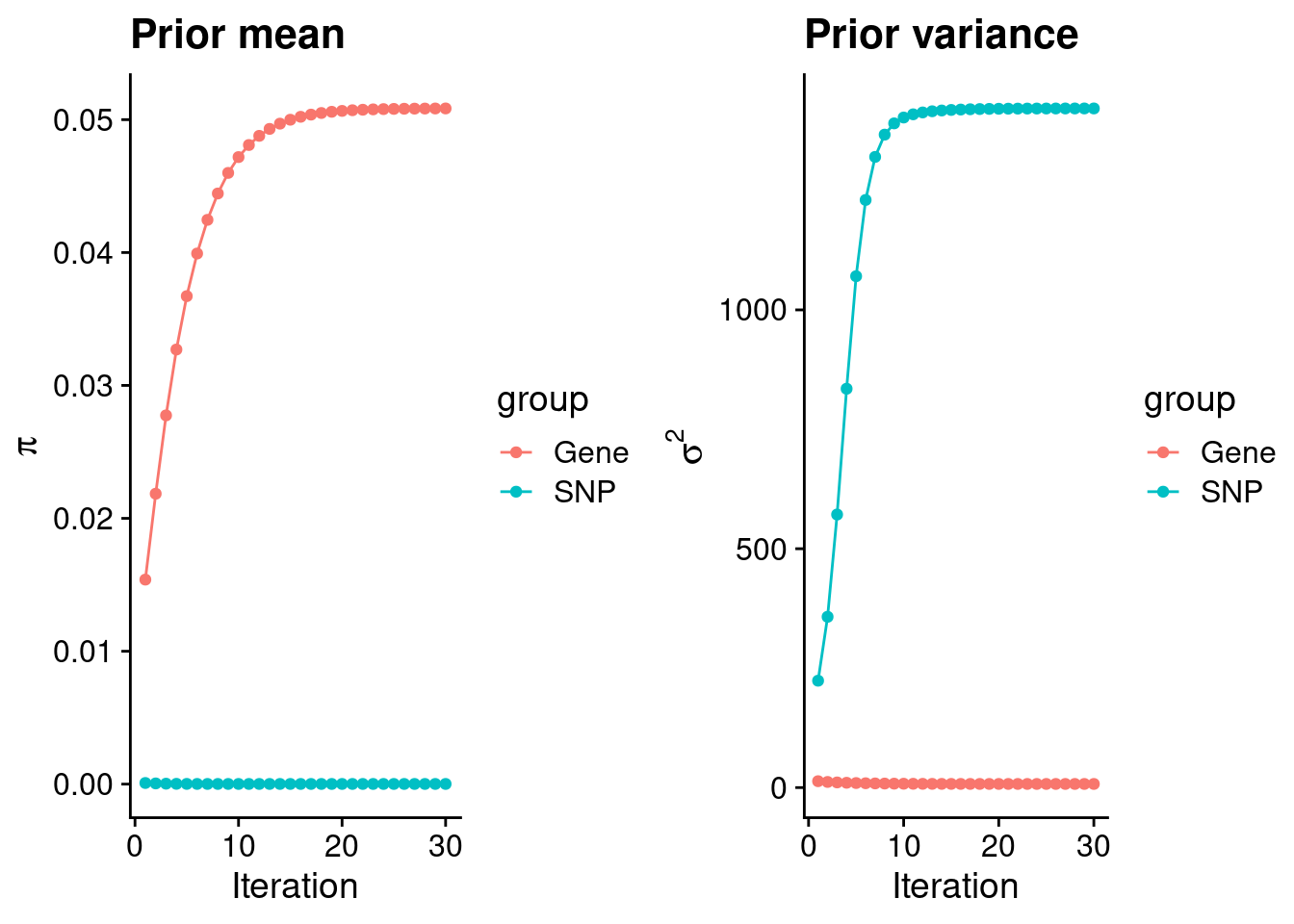
| Version | Author | Date |
|---|---|---|
| dfd2b5f | wesleycrouse | 2021-09-07 |
#estimated group prior
estimated_group_prior <- group_prior_rec[,ncol(group_prior_rec)]
names(estimated_group_prior) <- c("gene", "snp")
estimated_group_prior["snp"] <- estimated_group_prior["snp"]*thin #adjust parameter to account for thin argument
print(estimated_group_prior)
gene snp
5.084218e-02 1.302305e-05 #estimated group prior variance
estimated_group_prior_var <- group_prior_var_rec[,ncol(group_prior_var_rec)]
names(estimated_group_prior_var) <- c("gene", "snp")
print(estimated_group_prior_var) gene snp
7.61612 1421.72654 #report sample size
print(sample_size)[1] 342829#report group size
group_size <- c(nrow(ctwas_gene_res), n_snps)
print(group_size)[1] 10901 8697330#estimated group PVE
estimated_group_pve <- estimated_group_prior_var*estimated_group_prior*group_size/sample_size #check PVE calculation
names(estimated_group_pve) <- c("gene", "snp")
print(estimated_group_pve) gene snp
0.01231251 0.46971815 #compare sum(PIP*mu2/sample_size) with above PVE calculation
c(sum(ctwas_gene_res$PVE),sum(ctwas_snp_res$PVE))[1] 0.05863767 49.44282464Genes with highest PIPs
#distribution of PIPs
hist(ctwas_gene_res$susie_pip, xlim=c(0,1), main="Distribution of Gene PIPs")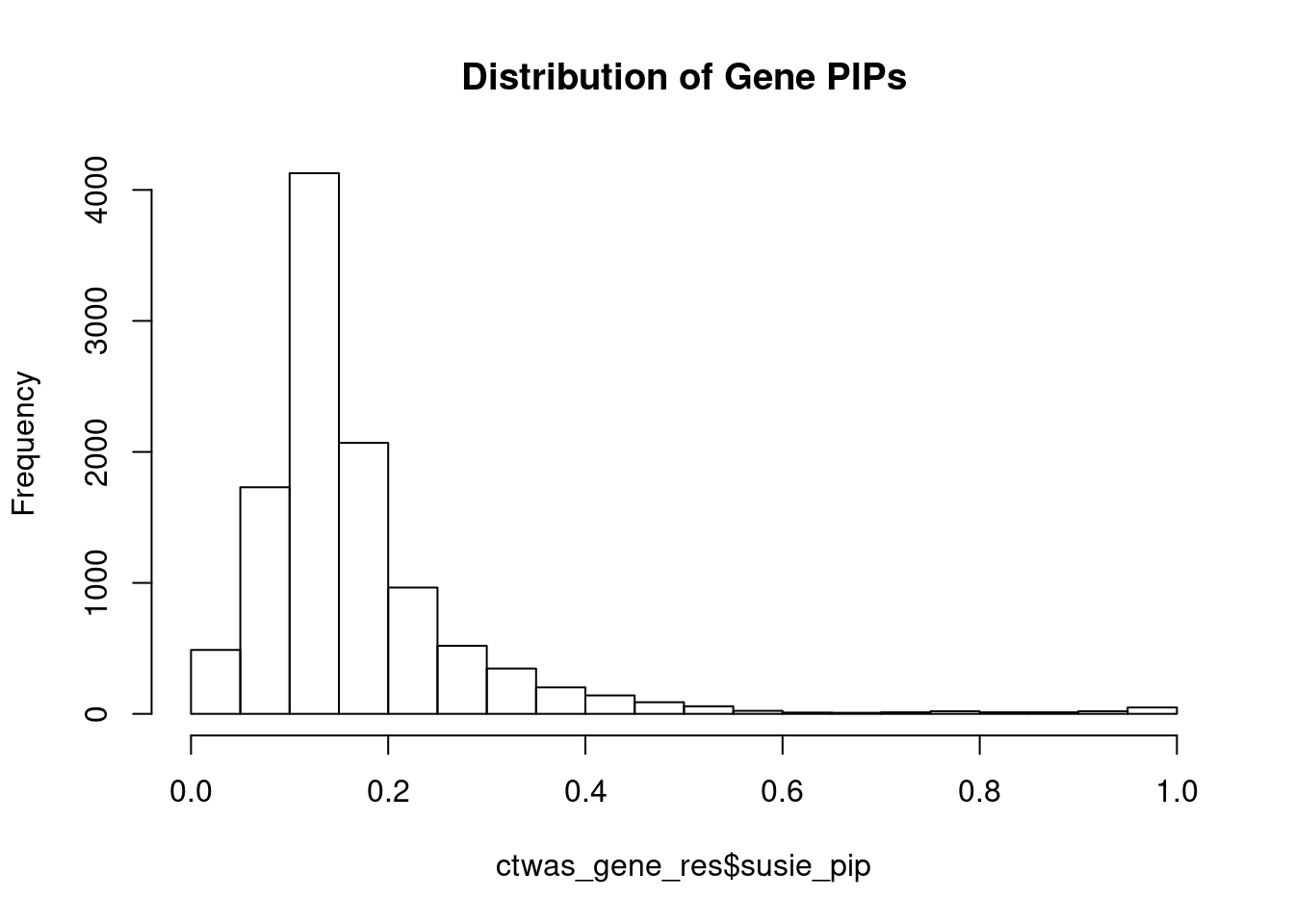
| Version | Author | Date |
|---|---|---|
| dfd2b5f | wesleycrouse | 2021-09-07 |
#genes with PIP>0.8 or 20 highest PIPs
head(ctwas_gene_res[order(-ctwas_gene_res$susie_pip),report_cols], max(sum(ctwas_gene_res$susie_pip>0.8), 20))
genename region_tag susie_pip mu2 PVE z
3212 CCND2 12_4 1.000 34.16 1.0e-04 6.06
6498 ITGAD 16_25 1.000 29.29 8.5e-05 3.24
9783 RHD 1_18 0.999 43.68 1.3e-04 -3.97
2809 COL7A1 3_35 0.999 27.32 8.0e-05 5.26
1231 PABPC4 1_24 0.998 43.09 1.3e-04 6.81
1320 CWF19L1 10_64 0.998 26.80 7.8e-05 -5.69
1848 CD276 15_35 0.998 27.90 8.1e-05 5.43
2050 DNASE2 19_10 0.998 27.20 7.9e-05 5.48
3385 TBX2 17_36 0.997 23.26 6.8e-05 4.80
9787 TMPRSS6 22_14 0.997 27.82 8.1e-05 1.99
7355 BRI3 7_60 0.996 37.49 1.1e-04 -6.42
6291 JAZF1 7_23 0.995 25.41 7.4e-05 5.11
6792 ADAR 1_75 0.993 23.42 6.8e-05 -5.92
12008 HPR 16_38 0.992 20.36 5.9e-05 -4.30
4269 ITGB4 17_42 0.992 23.46 6.8e-05 -5.24
10893 LINC02026 3_119 0.991 19.89 5.8e-05 -4.37
2508 KCTD10 12_66 0.991 22.33 6.5e-05 -4.55
8506 FAM222B 17_17 0.991 31.31 9.1e-05 5.86
6093 CSNK1G3 5_75 0.989 35.04 1.0e-04 6.23
583 ZNF76 6_28 0.988 23.13 6.7e-05 -4.85
7651 CASC4 15_17 0.988 20.98 6.0e-05 4.09
12467 RP11-219B17.3 15_27 0.988 90.90 2.6e-04 10.34
5415 SYTL1 1_19 0.987 19.07 5.5e-05 -4.26
12687 RP4-781K5.7 1_121 0.987 62.21 1.8e-04 -8.47
10212 IL27 16_23 0.987 46.52 1.3e-04 -7.78
10495 PRMT6 1_66 0.986 43.86 1.3e-04 6.84
2924 EFHD1 2_136 0.984 33.94 9.7e-05 7.18
7256 CEP44 4_113 0.983 20.80 6.0e-05 4.71
6411 LRGUK 7_81 0.983 19.41 5.6e-05 -4.32
4178 PDLIM4 5_79 0.982 31.76 9.1e-05 -6.38
5978 ZC3H12C 11_65 0.982 19.60 5.6e-05 -4.31
4275 EIF5A 17_6 0.981 24.31 7.0e-05 -5.03
669 ATP11A 13_61 0.980 19.38 5.5e-05 -4.28
7329 DAGLB 7_9 0.974 18.62 5.3e-05 4.25
2474 CBL 11_71 0.973 19.28 5.5e-05 -4.22
5991 FADS1 11_34 0.972 67.00 1.9e-04 8.84
4143 LILRB2 19_37 0.966 17.84 5.0e-05 4.00
2993 GPX7 1_33 0.965 16.88 4.7e-05 3.93
3562 ACVR1C 2_94 0.964 19.91 5.6e-05 4.42
10214 ZNF165 6_22 0.963 31.59 8.9e-05 8.63
6840 PCYT1A 3_121 0.962 17.96 5.0e-05 4.07
8811 SMIM19 8_37 0.961 49.82 1.4e-04 -7.52
4979 CARF 2_120 0.959 19.09 5.3e-05 -4.34
8190 ADORA2B 17_14 0.959 34.58 9.7e-05 6.21
8937 FAM20C 7_1 0.958 17.75 5.0e-05 4.02
10594 PSMB8 6_27 0.955 22.57 6.3e-05 -5.63
10496 SHISA4 1_102 0.953 16.82 4.7e-05 -3.66
5253 IRF8 16_50 0.953 17.68 4.9e-05 -3.96
5465 PRCC 1_77 0.952 28.27 7.8e-05 -5.65
9457 CBX6 22_15 0.950 18.02 5.0e-05 -4.04
1991 PIAS4 19_4 0.948 20.22 5.6e-05 4.53
5400 EPHA2 1_11 0.947 17.98 5.0e-05 -4.35
5658 ALDH1L1 3_78 0.947 17.01 4.7e-05 3.73
59 MPO 17_34 0.946 17.96 5.0e-05 4.25
12041 RP11-95P2.3 16_4 0.945 16.37 4.5e-05 -3.79
711 SMG6 17_3 0.942 27.35 7.5e-05 -3.95
3791 PROZ 13_62 0.941 17.02 4.7e-05 -3.87
8156 GYPA 4_94 0.935 20.70 5.6e-05 5.35
1982 PDCD5 19_23 0.933 16.69 4.5e-05 3.85
7266 HHIP 4_94 0.929 19.81 5.4e-05 -4.48
566 TNPO3 7_78 0.927 15.91 4.3e-05 3.67
6377 ANKRD40 17_29 0.926 16.77 4.5e-05 -3.84
3032 KIAA2013 1_9 0.922 17.54 4.7e-05 3.99
6926 ACOT11 1_34 0.919 16.22 4.3e-05 3.69
8150 ZNF778 16_54 0.916 15.71 4.2e-05 -3.57
4710 TTC5 14_1 0.910 16.07 4.3e-05 -3.62
3645 PEX6 6_33 0.904 40.59 1.1e-04 -6.63
5087 SLC38A4 12_29 0.904 17.43 4.6e-05 3.80
4813 KLC4 6_33 0.901 19.16 5.0e-05 -3.92
8493 OXSR1 3_27 0.900 16.68 4.4e-05 -3.73
4529 UBQLN1 9_41 0.896 20.10 5.3e-05 4.26
11149 OST4 2_16 0.894 18.67 4.9e-05 -4.57
8489 RNASEH2C 11_36 0.893 19.37 5.0e-05 4.27
537 DGAT2 11_42 0.892 65.38 1.7e-04 -8.54
2758 GNPDA1 5_84 0.880 16.32 4.2e-05 3.70
6699 GPBP1L1 1_28 0.878 21.86 5.6e-05 -4.58
8344 PLEKHG5 1_5 0.871 16.85 4.3e-05 -3.85
5724 GTF2H2 5_42 0.869 16.17 4.1e-05 3.58
666 COASY 17_25 0.868 17.38 4.4e-05 -3.87
10617 LAYN 11_66 0.866 20.44 5.2e-05 5.16
7304 UTP15 5_43 0.851 16.37 4.1e-05 -3.53
1408 SF3A1 22_10 0.846 20.60 5.1e-05 -4.77
8142 CNTROB 17_7 0.845 37.67 9.3e-05 -6.57
9374 SPATA13 13_5 0.834 16.89 4.1e-05 -3.57
5782 MMS22L 6_66 0.832 17.30 4.2e-05 -3.66
10195 ABCB8 7_94 0.828 16.44 4.0e-05 3.52
5231 ARMC5 16_25 0.827 22.93 5.5e-05 -1.29
11254 LINC00472 6_50 0.825 17.00 4.1e-05 3.54
11520 TMEM199 17_17 0.824 15.48 3.7e-05 3.25
9729 GLDN 15_20 0.820 16.96 4.1e-05 3.65
7513 CYP2C19 10_61 0.818 49.10 1.2e-04 -7.48
3364 SOCS2 12_55 0.808 17.12 4.0e-05 -3.56
2906 RTN4 2_36 0.802 16.44 3.8e-05 3.29Genes with largest effect sizes
#plot PIP vs effect size
plot(ctwas_gene_res$susie_pip, ctwas_gene_res$mu2, xlab="PIP", ylab="mu^2", main="Gene PIPs vs Effect Size")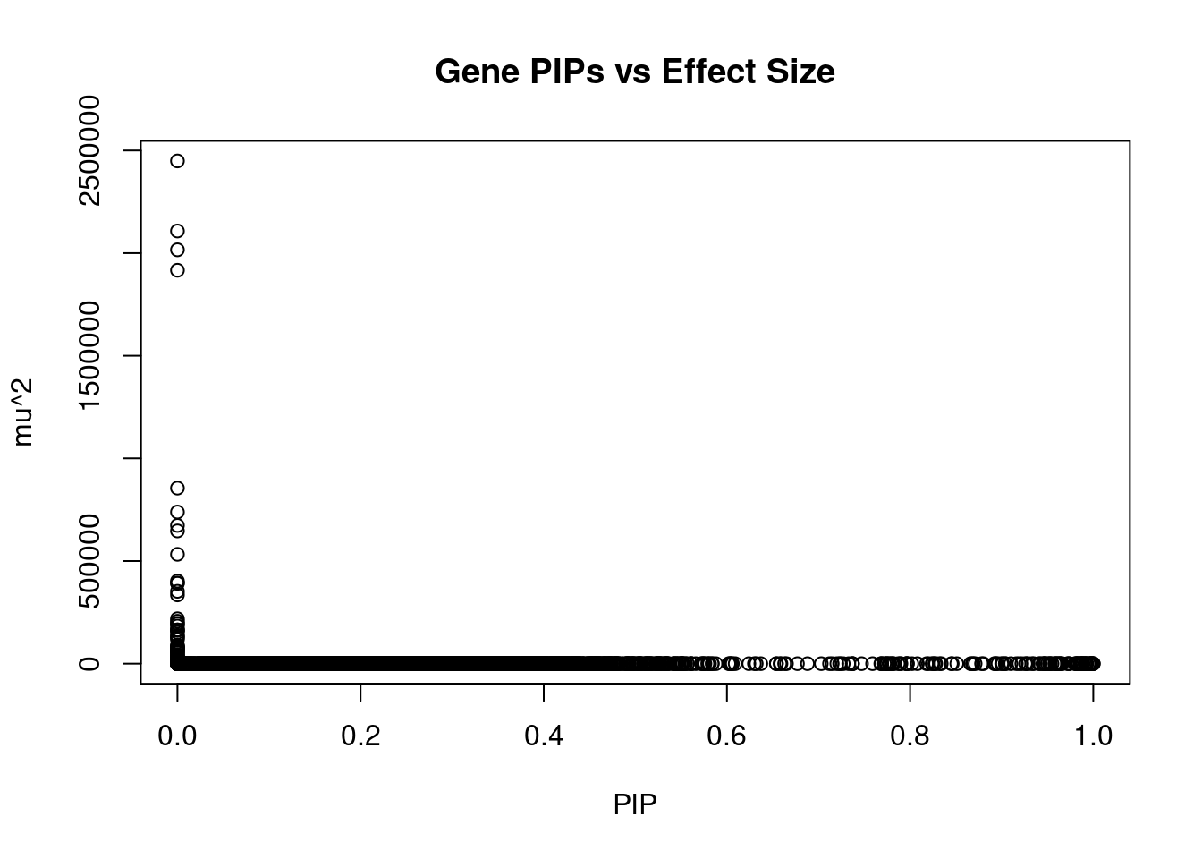
| Version | Author | Date |
|---|---|---|
| dfd2b5f | wesleycrouse | 2021-09-07 |
#genes with 20 largest effect sizes
head(ctwas_gene_res[order(-ctwas_gene_res$mu2),report_cols],20)
genename region_tag susie_pip mu2 PVE z
11533 UGT1A4 2_137 0 2448970.2 0 304.19
11489 UGT1A3 2_137 0 2107677.6 0 265.38
11447 UGT1A1 2_137 0 2016066.4 0 -298.45
7732 UGT1A6 2_137 0 1916403.2 0 230.23
10602 RNF5 6_26 0 855192.6 0 7.70
11007 PPT2 6_26 0 738649.7 0 -6.65
12683 HCP5B 6_24 0 673465.6 0 -6.62
10848 CLIC1 6_26 0 646598.3 0 7.41
11541 C4A 6_26 0 532580.0 0 6.27
10601 AGER 6_26 0 402686.6 0 -0.26
10599 NOTCH4 6_26 0 392520.7 0 9.20
11522 UGT1A7 2_137 0 391584.5 0 -82.75
10663 TRIM31 6_24 0 352477.6 0 4.25
4833 FLOT1 6_24 0 334856.6 0 -5.78
10626 MPIG6B 6_26 0 218823.1 0 -1.76
10849 DDAH2 6_26 0 206664.9 0 8.88
10625 MSH5 6_26 0 196186.7 0 4.00
10603 AGPAT1 6_26 0 193435.2 0 -7.76
10137 HLA-DQA1 6_26 0 183023.5 0 4.90
10616 EHMT2 6_26 0 164615.1 0 3.18Genes with highest PVE
#genes with 20 highest pve
head(ctwas_gene_res[order(-ctwas_gene_res$PVE),report_cols],20)
genename region_tag susie_pip mu2 PVE z
12467 RP11-219B17.3 15_27 0.988 90.90 2.6e-04 10.34
5991 FADS1 11_34 0.972 67.00 1.9e-04 8.84
12687 RP4-781K5.7 1_121 0.987 62.21 1.8e-04 -8.47
537 DGAT2 11_42 0.892 65.38 1.7e-04 -8.54
8811 SMIM19 8_37 0.961 49.82 1.4e-04 -7.52
9783 RHD 1_18 0.999 43.68 1.3e-04 -3.97
1231 PABPC4 1_24 0.998 43.09 1.3e-04 6.81
10495 PRMT6 1_66 0.986 43.86 1.3e-04 6.84
10212 IL27 16_23 0.987 46.52 1.3e-04 -7.78
7513 CYP2C19 10_61 0.818 49.10 1.2e-04 -7.48
3645 PEX6 6_33 0.904 40.59 1.1e-04 -6.63
7355 BRI3 7_60 0.996 37.49 1.1e-04 -6.42
6093 CSNK1G3 5_75 0.989 35.04 1.0e-04 6.23
3212 CCND2 12_4 1.000 34.16 1.0e-04 6.06
4317 ANGPTL3 1_39 0.654 52.06 9.9e-05 7.74
2924 EFHD1 2_136 0.984 33.94 9.7e-05 7.18
8190 ADORA2B 17_14 0.959 34.58 9.7e-05 6.21
8142 CNTROB 17_7 0.845 37.67 9.3e-05 -6.57
4178 PDLIM4 5_79 0.982 31.76 9.1e-05 -6.38
8506 FAM222B 17_17 0.991 31.31 9.1e-05 5.86Genes with largest z scores
#genes with 20 largest z scores
head(ctwas_gene_res[order(-abs(ctwas_gene_res$z)),report_cols],20)
genename region_tag susie_pip mu2 PVE z
11533 UGT1A4 2_137 0.000 2448970.25 0.0e+00 304.19
11447 UGT1A1 2_137 0.000 2016066.37 0.0e+00 -298.45
11489 UGT1A3 2_137 0.000 2107677.62 0.0e+00 265.38
7732 UGT1A6 2_137 0.000 1916403.22 0.0e+00 230.23
11522 UGT1A7 2_137 0.000 391584.48 0.0e+00 -82.75
1088 USP40 2_137 0.000 126387.43 0.0e+00 -56.37
3556 HJURP 2_137 0.000 15983.38 0.0e+00 13.62
8651 MSL2 3_84 0.131 135.27 5.2e-05 13.00
10747 SLCO1B7 12_16 0.000 1123.81 0.0e+00 10.94
2584 SLCO1B3 12_16 0.000 573.23 0.0e+00 10.75
12467 RP11-219B17.3 15_27 0.988 90.90 2.6e-04 10.34
9829 ZKSCAN4 6_22 0.050 43.54 6.3e-06 -9.67
10599 NOTCH4 6_26 0.000 392520.70 0.0e+00 9.20
10849 DDAH2 6_26 0.000 206664.87 0.0e+00 8.88
5991 FADS1 11_34 0.972 67.00 1.9e-04 8.84
11290 MAPKAPK5-AS1 12_67 0.228 54.89 3.6e-05 -8.70
10214 ZNF165 6_22 0.963 31.59 8.9e-05 8.63
537 DGAT2 11_42 0.892 65.38 1.7e-04 -8.54
2170 AHR 7_17 0.135 55.75 2.2e-05 -8.51
10374 ZKSCAN8 6_22 0.039 26.08 2.9e-06 -8.49Comparing z scores and PIPs
#set nominal signifiance threshold for z scores
alpha <- 0.05

#bonferroni adjusted threshold for z scores
sig_thresh <- qnorm(1-(alpha/nrow(ctwas_gene_res)/2), lower=T)

#Q-Q plot for z scores
obs_z <- ctwas_gene_res$z[order(ctwas_gene_res$z)]
exp_z <- qnorm((1:nrow(ctwas_gene_res))/nrow(ctwas_gene_res))

plot(exp_z, obs_z, xlab="Expected z", ylab="Observed z", main="Gene z score Q-Q plot")
abline(a=0,b=1)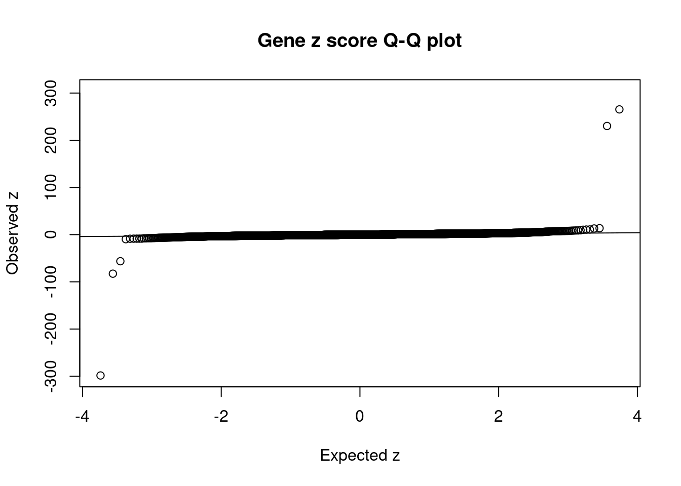
| Version | Author | Date |
|---|---|---|
| dfd2b5f | wesleycrouse | 2021-09-07 |
#plot z score vs PIP
plot(abs(ctwas_gene_res$z), ctwas_gene_res$susie_pip, xlab="abs(z)", ylab="PIP")
abline(v=sig_thresh, col="red", lty=2)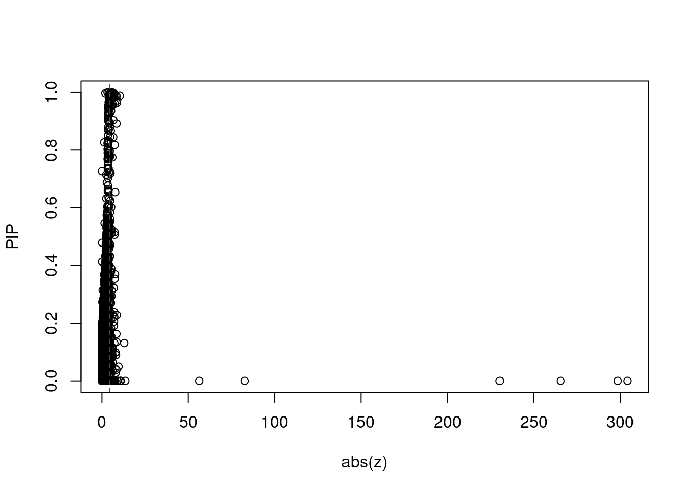
| Version | Author | Date |
|---|---|---|
| dfd2b5f | wesleycrouse | 2021-09-07 |
#proportion of significant z scores
mean(abs(ctwas_gene_res$z) > sig_thresh)
[1] 0.01467755#genes with most significant z scores
head(ctwas_gene_res[order(-abs(ctwas_gene_res$z)),report_cols],20) genename region_tag susie_pip mu2 PVE z
11533 UGT1A4 2_137 0.000 2448970.25 0.0e+00 304.19
11447 UGT1A1 2_137 0.000 2016066.37 0.0e+00 -298.45
11489 UGT1A3 2_137 0.000 2107677.62 0.0e+00 265.38
7732 UGT1A6 2_137 0.000 1916403.22 0.0e+00 230.23
11522 UGT1A7 2_137 0.000 391584.48 0.0e+00 -82.75
1088 USP40 2_137 0.000 126387.43 0.0e+00 -56.37
3556 HJURP 2_137 0.000 15983.38 0.0e+00 13.62
8651 MSL2 3_84 0.131 135.27 5.2e-05 13.00
10747 SLCO1B7 12_16 0.000 1123.81 0.0e+00 10.94
2584 SLCO1B3 12_16 0.000 573.23 0.0e+00 10.75
12467 RP11-219B17.3 15_27 0.988 90.90 2.6e-04 10.34
9829 ZKSCAN4 6_22 0.050 43.54 6.3e-06 -9.67
10599 NOTCH4 6_26 0.000 392520.70 0.0e+00 9.20
10849 DDAH2 6_26 0.000 206664.87 0.0e+00 8.88
5991 FADS1 11_34 0.972 67.00 1.9e-04 8.84
11290 MAPKAPK5-AS1 12_67 0.228 54.89 3.6e-05 -8.70
10214 ZNF165 6_22 0.963 31.59 8.9e-05 8.63
537 DGAT2 11_42 0.892 65.38 1.7e-04 -8.54
2170 AHR 7_17 0.135 55.75 2.2e-05 -8.51
10374 ZKSCAN8 6_22 0.039 26.08 2.9e-06 -8.49Locus plots for genes and SNPs
ctwas_gene_res_sortz <- ctwas_gene_res[order(-abs(ctwas_gene_res$z)),]

n_plots <- 5
for (region_tag_plot in head(unique(ctwas_gene_res_sortz$region_tag), n_plots)){
  ctwas_res_region <-  ctwas_res[ctwas_res$region_tag==region_tag_plot,]
  start <- min(ctwas_res_region$pos)
  end <- max(ctwas_res_region$pos)

  ctwas_res_region <- ctwas_res_region[order(ctwas_res_region$pos),]
  ctwas_res_region_gene <- ctwas_res_region[ctwas_res_region$type=="gene",]
  ctwas_res_region_snp <- ctwas_res_region[ctwas_res_region$type=="SNP",]

  #region name
  print(paste0("Region: ", region_tag_plot))

  #table of genes in region
  print(ctwas_res_region_gene[,report_cols])

  par(mfrow=c(4,1))

  #gene z scores
  plot(ctwas_res_region_gene$pos, abs(ctwas_res_region_gene$z), xlab="Position", ylab="abs(gene_z)", xlim=c(start,end),
   ylim=c(0,max(sig_thresh, abs(ctwas_res_region_gene$z))),
   main=paste0("Region: ", region_tag_plot))
  abline(h=sig_thresh,col="red",lty=2)

  #significance threshold for SNPs
  alpha_snp <- 5*10^(-8)
  sig_thresh_snp <- qnorm(1-alpha_snp/2, lower=T)

  #snp z scores
  plot(ctwas_res_region_snp$pos, abs(ctwas_res_region_snp$z), xlab="Position", ylab="abs(snp_z)",xlim=c(start,end),
   ylim=c(0,max(sig_thresh_snp, max(abs(ctwas_res_region_snp$z)))))
  abline(h=sig_thresh_snp,col="purple",lty=2)

  #gene pips
  plot(ctwas_res_region_gene$pos, ctwas_res_region_gene$susie_pip, xlab="Position", ylab="Gene PIP", xlim=c(start,end), ylim=c(0,1))
  abline(h=0.8,col="blue",lty=2)

  #snp pips
  plot(ctwas_res_region_snp$pos, ctwas_res_region_snp$susie_pip, xlab="Position", ylab="SNP PIP", xlim=c(start,end), ylim=c(0,1))
  abline(h=0.8,col="blue",lty=2)
}
[1] "Region: 2_137"
genename region_tag susie_pip mu2 PVE z
10567 GIGYF2 2_137 0 2358.96 0 -7.32
9340 C2orf82 2_137 0 18.43 0 0.49
620 NGEF 2_137 0 544.24 0 2.98
8006 INPP5D 2_137 0 596.32 0 5.74
879 DGKD 2_137 0 5148.05 0 0.77
1088 USP40 2_137 0 126387.43 0 -56.37
11522 UGT1A7 2_137 0 391584.48 0 -82.75
7732 UGT1A6 2_137 0 1916403.22 0 230.23
11533 UGT1A4 2_137 0 2448970.25 0 304.19
11489 UGT1A3 2_137 0 2107677.62 0 265.38
11447 UGT1A1 2_137 0 2016066.37 0 -298.45
3556 HJURP 2_137 0 15983.38 0 13.62
11098 AC006037.2 2_137 0 55.25 0 0.70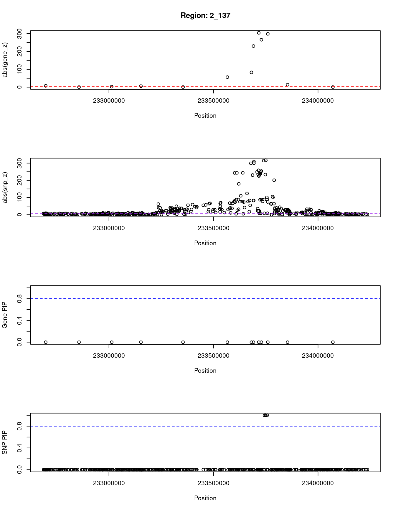
| Version | Author | Date |
|---|---|---|
| dfd2b5f | wesleycrouse | 2021-09-07 |
[1] "Region: 3_84"
     genename region_tag susie_pip    mu2     PVE     z
796   PPP2R3A       3_84     0.318  20.39 1.9e-05 -3.21
8651     MSL2       3_84     0.131 135.27 5.2e-05 13.00
2795     PCCB       3_84     0.118   8.10 2.8e-06  0.60
3148    STAG1       3_84     0.081   5.02 1.2e-06  0.96
6584     NCK1       3_84     0.120  10.93 3.8e-06 -1.83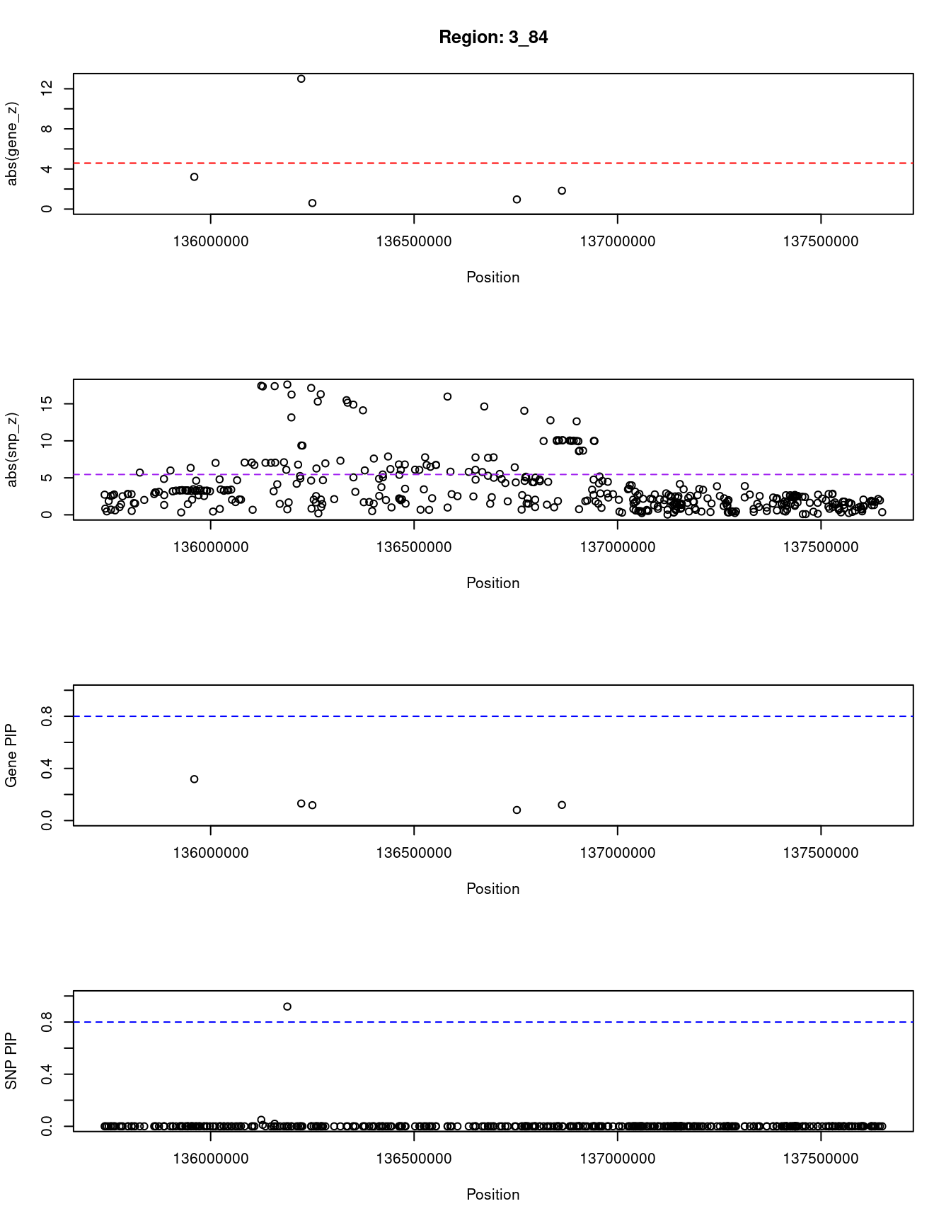
| Version | Author | Date |
|---|---|---|
| dfd2b5f | wesleycrouse | 2021-09-07 |
[1] "Region: 12_16"
      genename region_tag susie_pip     mu2 PVE     z
2584   SLCO1B3      12_16         0  573.23   0 10.75
10747  SLCO1B7      12_16         0 1123.81   0 10.94
3400      IAPP      12_16         0  176.25   0  7.16
3399   PYROXD1      12_16         0   19.99   0  0.97
36       RECQL      12_16         0  279.30   0  6.62
2586    GOLT1B      12_16         0   42.16   0  6.79
4482       SPX      12_16         0  301.54   0  7.14
2587      LDHB      12_16         0    6.26   0  0.86
3401     KCNJ8      12_16         0    9.95   0  0.19
689      ABCC9      12_16         0    8.57   0  3.17
2590     C2CD5      12_16         0    6.01   0 -0.73
5073     ETNK1      12_16         0   35.98   0  1.89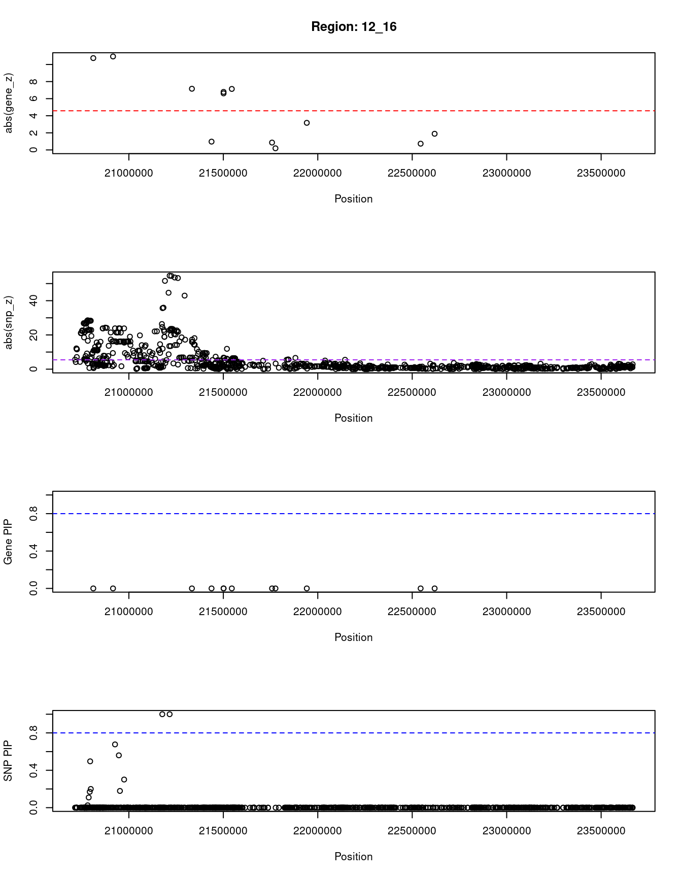
| Version | Author | Date |
|---|---|---|
| dfd2b5f | wesleycrouse | 2021-09-07 |
[1] "Region: 15_27"
           genename region_tag susie_pip   mu2     PVE     z
5185          GCNT3      15_27     0.079  4.80 1.1e-06 -0.28
5186         GTF2A2      15_27     0.226 14.31 9.4e-06 -1.85
3965           ICE2      15_27     0.093 14.41 3.9e-06 -3.36
12467 RP11-219B17.3      15_27     0.988 90.90 2.6e-04 10.34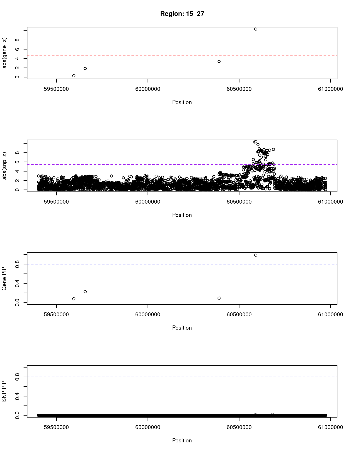
| Version | Author | Date |
|---|---|---|
| dfd2b5f | wesleycrouse | 2021-09-07 |
[1] "Region: 6_22"
      genename region_tag susie_pip   mu2     PVE     z
10214   ZNF165       6_22     0.963 31.59 8.9e-05  8.63
10145  ZSCAN16       6_22     0.035  4.78 4.9e-07 -0.60
10374  ZKSCAN8       6_22     0.039 26.08 2.9e-06 -8.49
4815    ZSCAN9       6_22     0.035  5.62 5.7e-07  1.27
9829   ZKSCAN4       6_22     0.050 43.54 6.3e-06 -9.67
9991     NKAPL       6_22     0.109 33.89 1.1e-05 -6.20
10183  ZSCAN26       6_22     0.043 22.82 2.9e-06  7.77
10000  ZKSCAN3       6_22     0.624 21.81 4.0e-05  4.85
11307  ZSCAN31       6_22     0.108 11.68 3.7e-06 -3.89
6623   ZSCAN12       6_22     0.057 18.13 3.0e-06 -5.35
11219    ZBED9       6_22     0.037 11.93 1.3e-06  1.89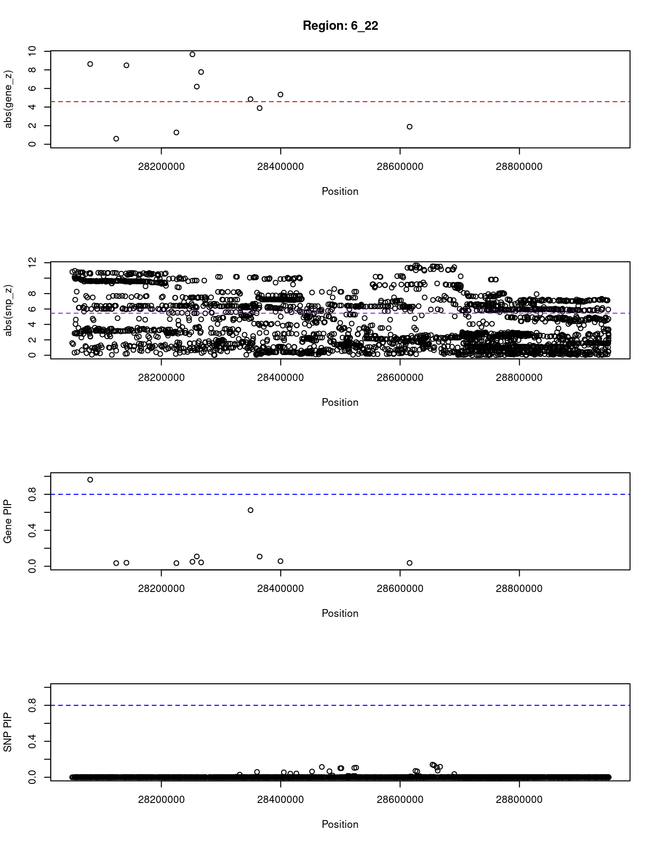
| Version | Author | Date |
|---|---|---|
| dfd2b5f | wesleycrouse | 2021-09-07 |
SNPs with highest PIPs
#snps with PIP>0.8 or 20 highest PIPs
head(ctwas_snp_res[order(-ctwas_snp_res$susie_pip),report_cols_snps],
max(sum(ctwas_snp_res$susie_pip>0.8), 20))
id region_tag susie_pip mu2 PVE z
58327 rs12239046 1_131 1.000 47.18 1.4e-04 -6.51
126267 rs76063448 2_137 1.000 64944.54 1.9e-01 87.93
126268 rs11888459 2_137 1.000 3514921.84 1.0e+01 233.42
126269 rs2885296 2_137 1.000 3334408.63 9.7e+00 316.17
126271 rs11568318 2_137 1.000 862446.95 2.5e+00 -89.02
313867 rs72834643 6_20 1.000 204.50 6.0e-04 12.21
313888 rs115740542 6_20 1.000 257.65 7.5e-04 14.39
364503 rs542176135 7_17 1.000 251.19 7.3e-04 -10.36
511870 rs6480402 10_46 1.000 995.88 2.9e-03 11.91
577598 rs11045819 12_16 1.000 5698.70 1.7e-02 -24.62
577615 rs4363657 12_16 1.000 2505.24 7.3e-03 54.59
603204 rs653178 12_67 1.000 232.79 6.8e-04 -15.66
762475 rs59616136 19_14 1.000 61.47 1.8e-04 8.30
919247 rs34247311 2_136 1.000 70.67 2.1e-04 5.97
919310 rs13031505 2_136 1.000 105.73 3.1e-04 -10.34
995706 rs1611236 6_24 1.000 1799666.12 5.2e+00 -5.01
1006891 rs199859210 6_26 1.000 3793.99 1.1e-02 -1.16
1006954 rs3130292 6_26 1.000 1707075.71 5.0e+00 -8.33
1006965 rs9279507 6_26 1.000 1707072.87 5.0e+00 0.17
1093349 rs766880753 8_73 1.000 97055.98 2.8e-01 4.06
1101316 rs201623796 10_6 1.000 110950.15 3.2e-01 -3.78
1101324 rs186871467 10_6 1.000 12584.19 3.7e-02 2.33
1275107 rs138395719 17_23 1.000 64385.37 1.9e-01 -3.58
1318478 rs112896133 19_10 0.998 56.19 1.6e-04 -7.17
532644 rs76153913 11_2 0.997 44.98 1.3e-04 6.13
31315 rs2779116 1_78 0.996 154.54 4.5e-04 -12.25
532658 rs118092312 11_2 0.994 55.36 1.6e-04 -2.24
715889 rs2608604 16_53 0.994 94.03 2.7e-04 -7.55
488217 rs34755157 9_71 0.992 46.72 1.4e-04 -6.53
1344077 rs855791 22_14 0.992 185.32 5.4e-04 12.34
770397 rs814573 19_32 0.990 40.63 1.2e-04 5.98
422740 rs12550646 8_36 0.989 52.69 1.5e-04 7.32
577353 rs10770693 12_15 0.989 97.20 2.8e-04 10.67
786716 rs6129760 20_25 0.989 63.65 1.8e-04 7.10
126457 rs6431241 2_138 0.988 45.41 1.3e-04 -7.18
586773 rs10876377 12_33 0.981 46.68 1.3e-04 6.21
126472 rs72982172 2_138 0.978 38.72 1.1e-04 -4.20
364525 rs4721597 7_17 0.976 145.92 4.2e-04 1.77
314509 rs559462124 6_23 0.975 64.82 1.8e-04 -8.19
473750 rs9410381 9_45 0.970 91.57 2.6e-04 9.34
88899 rs1992769 2_58 0.968 36.45 1.0e-04 -5.62
313732 rs72838866 6_19 0.961 101.00 2.8e-04 10.46
74479 rs10495928 2_28 0.958 37.19 1.0e-04 -5.66
763260 rs3794991 19_15 0.957 66.21 1.8e-04 7.93
534829 rs4910498 11_8 0.951 49.26 1.4e-04 6.55
366098 rs56130071 7_19 0.942 73.61 2.0e-04 8.31
536258 rs10766077 11_10 0.937 57.85 1.6e-04 7.28
1122385 rs11601507 11_4 0.924 45.93 1.2e-04 6.41
169833 rs6779146 3_84 0.919 311.27 8.3e-04 17.61
587687 rs2657880 12_35 0.912 40.30 1.1e-04 5.92
655489 rs873642 14_30 0.911 36.99 9.8e-05 -5.54
511879 rs73267631 10_46 0.907 260.96 6.9e-04 -1.46
1101295 rs4880705 10_6 0.904 111797.08 2.9e-01 -5.40
224979 rs17238095 4_72 0.897 43.01 1.1e-04 6.31
487832 rs115478735 9_70 0.897 55.05 1.4e-04 -7.00
417398 rs35469695 8_24 0.885 40.91 1.1e-04 6.01
715837 rs8044367 16_53 0.883 51.64 1.3e-04 3.68
474431 rs290992 9_46 0.874 37.08 9.5e-05 -6.09
1101304 rs7914015 10_6 0.864 111676.29 2.8e-01 -5.35
307142 rs2765359 6_7 0.834 41.50 1.0e-04 6.03
314457 rs149972 6_21 0.826 126.27 3.0e-04 -10.99
560861 rs11224303 11_58 0.819 38.53 9.2e-05 5.77
577313 rs7962574 12_15 0.810 71.53 1.7e-04 -9.30SNPs with largest effect sizes
#plot PIP vs effect size
plot(ctwas_snp_res$susie_pip, ctwas_snp_res$mu2, xlab="PIP", ylab="mu^2", main="SNP PIPs vs Effect Size")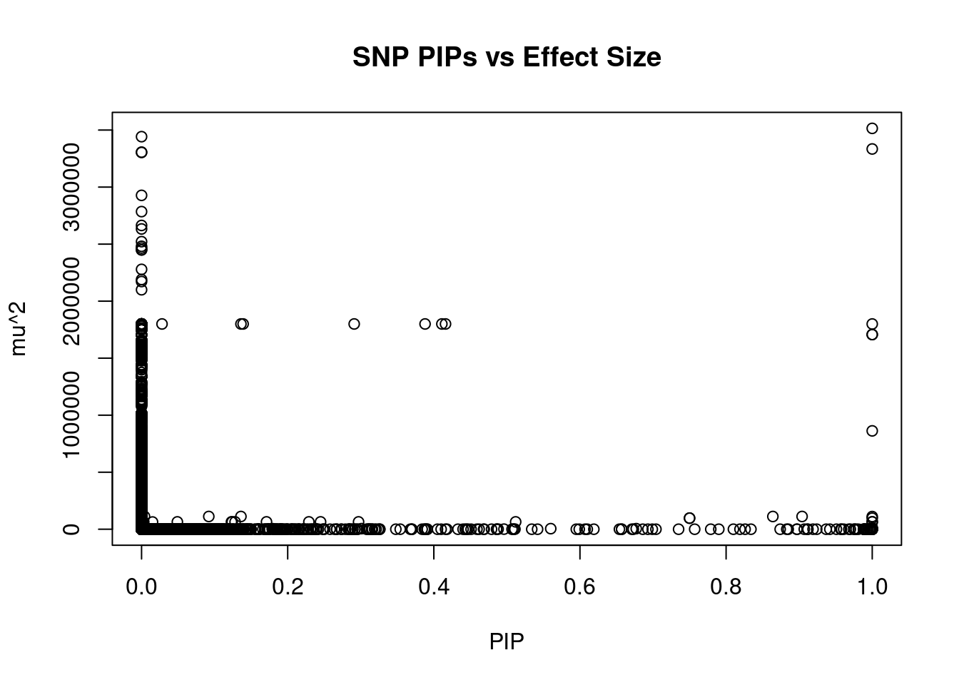
| Version | Author | Date |
|---|---|---|
| dfd2b5f | wesleycrouse | 2021-09-07 |
#SNPs with 50 largest effect sizes
head(ctwas_snp_res[order(-ctwas_snp_res$mu2),report_cols_snps],50)
id region_tag susie_pip mu2 PVE z
126268 rs11888459 2_137 1.000 3514922 1.0e+01 233.42
126251 rs13401281 2_137 0.000 3442241 0.0e+00 231.28
126269 rs2885296 2_137 1.000 3334409 9.7e+00 316.17
126265 rs17862875 2_137 0.000 3306447 0.0e+00 314.44
126248 rs1875263 2_137 0.000 3303886 0.0e+00 225.15
126247 rs6749496 2_137 0.000 2927567 0.0e+00 258.20
126240 rs7583278 2_137 0.000 2785042 0.0e+00 248.73
126256 rs4663332 2_137 0.000 2663747 0.0e+00 240.16
126257 rs200973045 2_137 0.000 2632987 0.0e+00 239.38
126258 rs57258852 2_137 0.000 2521666 0.0e+00 248.23
126262 rs3821242 2_137 0.000 2480837 0.0e+00 253.70
126260 rs2008584 2_137 0.000 2465187 0.0e+00 252.98
126234 rs6753320 2_137 0.000 2449406 0.0e+00 230.24
126235 rs6736743 2_137 0.000 2449406 0.0e+00 230.24
126239 rs2070959 2_137 0.000 2278621 0.0e+00 308.88
126238 rs1105880 2_137 0.000 2189390 0.0e+00 299.78
126233 rs77070100 2_137 0.000 2171928 0.0e+00 298.67
126246 rs2012734 2_137 0.000 2099773 0.0e+00 234.28
995688 rs111734624 6_24 0.416 1799890 2.2e+00 -5.03
995685 rs2508055 6_24 0.411 1799890 2.2e+00 -5.03
995733 rs1611252 6_24 0.291 1799889 1.5e+00 -5.03
995729 rs1611248 6_24 0.388 1799884 2.0e+00 -5.04
995750 rs1611260 6_24 0.139 1799883 7.3e-01 -5.03
995756 rs1611265 6_24 0.136 1799881 7.2e-01 -5.03
995624 rs1633033 6_24 0.028 1799847 1.4e-01 -5.04
995760 rs2394171 6_24 0.000 1799844 5.4e-07 -5.02
995758 rs1611267 6_24 0.000 1799842 3.4e-09 -5.01
995762 rs2893981 6_24 0.000 1799840 3.7e-07 -5.02
995692 rs1611228 6_24 0.000 1799836 2.2e-06 -5.02
995681 rs1737020 6_24 0.000 1799835 3.4e-11 -5.01
995682 rs1737019 6_24 0.000 1799835 3.4e-11 -5.01
995637 rs2844838 6_24 0.000 1799830 1.0e-03 -5.03
995641 rs1633032 6_24 0.000 1799715 3.9e-11 -5.03
995706 rs1611236 6_24 1.000 1799666 5.2e+00 -5.01
995675 rs1633020 6_24 0.000 1799616 0.0e+00 -5.01
995679 rs1633018 6_24 0.000 1799602 0.0e+00 -5.00
995704 rs1611234 6_24 0.000 1799493 0.0e+00 -5.00
995564 rs1610726 6_24 0.000 1799396 0.0e+00 -5.01
995632 rs2844840 6_24 0.000 1799214 0.0e+00 -5.04
995959 rs3129185 6_24 0.000 1799148 0.0e+00 -5.06
995974 rs1736999 6_24 0.000 1799072 0.0e+00 -5.06
995987 rs1633001 6_24 0.000 1798920 0.0e+00 -5.05
995727 rs1611246 6_24 0.000 1798903 0.0e+00 -5.02
996163 rs1632980 6_24 0.000 1798811 0.0e+00 -5.07
995660 rs1614309 6_24 0.000 1798360 0.0e+00 -5.04
995659 rs1633030 6_24 0.000 1796894 0.0e+00 -5.05
995772 rs9258382 6_24 0.000 1794984 0.0e+00 -5.04
995769 rs9258379 6_24 0.000 1792080 0.0e+00 -5.07
995718 rs1611241 6_24 0.000 1789879 0.0e+00 -5.12
995663 rs1633028 6_24 0.000 1787420 0.0e+00 -4.98SNPs with highest PVE
#SNPs with 50 highest pve
head(ctwas_snp_res[order(-ctwas_snp_res$PVE),report_cols_snps],50)
id region_tag susie_pip mu2 PVE z
126268 rs11888459 2_137 1.000 3514921.84 1.0e+01 233.42
126269 rs2885296 2_137 1.000 3334408.63 9.7e+00 316.17
995706 rs1611236 6_24 1.000 1799666.12 5.2e+00 -5.01
1006954 rs3130292 6_26 1.000 1707075.71 5.0e+00 -8.33
1006965 rs9279507 6_26 1.000 1707072.87 5.0e+00 0.17
126271 rs11568318 2_137 1.000 862446.95 2.5e+00 -89.02
995685 rs2508055 6_24 0.411 1799889.69 2.2e+00 -5.03
995688 rs111734624 6_24 0.416 1799889.98 2.2e+00 -5.03
995729 rs1611248 6_24 0.388 1799884.29 2.0e+00 -5.04
995733 rs1611252 6_24 0.291 1799888.97 1.5e+00 -5.03
995750 rs1611260 6_24 0.139 1799883.11 7.3e-01 -5.03
995756 rs1611265 6_24 0.136 1799881.35 7.2e-01 -5.03
1101316 rs201623796 10_6 1.000 110950.15 3.2e-01 -3.78
1101295 rs4880705 10_6 0.904 111797.08 2.9e-01 -5.40
1093349 rs766880753 8_73 1.000 97055.98 2.8e-01 4.06
1101304 rs7914015 10_6 0.864 111676.29 2.8e-01 -5.35
1093338 rs375646 8_73 0.750 97318.15 2.1e-01 4.40
1093339 rs441617 8_73 0.750 97318.15 2.1e-01 4.40
126267 rs76063448 2_137 1.000 64944.54 1.9e-01 87.93
1275107 rs138395719 17_23 1.000 64385.37 1.9e-01 -3.58
995624 rs1633033 6_24 0.028 1799846.73 1.4e-01 -5.04
1275106 rs9893520 17_23 0.512 64486.11 9.6e-02 -3.48
1275111 rs9897092 17_23 0.297 64484.99 5.6e-02 -3.48
1275076 rs9916782 17_23 0.245 64468.21 4.6e-02 -3.52
1101307 rs4644565 10_6 0.136 111626.37 4.4e-02 -5.34
1275075 rs16965687 17_23 0.229 64467.71 4.3e-02 -3.52
1101324 rs186871467 10_6 1.000 12584.19 3.7e-02 2.33
1275077 rs79880154 17_23 0.171 64483.26 3.2e-02 -3.49
1101294 rs7907985 10_6 0.092 111786.54 3.0e-02 -5.40
1275062 rs7359537 17_23 0.128 64480.85 2.4e-02 -3.49
1275065 rs9892404 17_23 0.124 64480.89 2.3e-02 -3.49
1275069 rs9906409 17_23 0.123 64481.00 2.3e-02 -3.49
577598 rs11045819 12_16 1.000 5698.70 1.7e-02 -24.62
1006891 rs199859210 6_26 1.000 3793.99 1.1e-02 -1.16
577499 rs12366506 12_16 0.677 5055.09 1.0e-02 23.86
1275055 rs72836642 17_23 0.049 64466.82 9.2e-03 -3.50
577505 rs11045612 12_16 0.560 5050.78 8.3e-03 23.88
577615 rs4363657 12_16 1.000 2505.24 7.3e-03 54.59
577516 rs73062442 12_16 0.301 5055.57 4.4e-03 23.83
511870 rs6480402 10_46 1.000 995.88 2.9e-03 11.91
1275058 rs58989731 17_23 0.015 63485.56 2.8e-03 -3.33
577508 rs11513221 12_16 0.179 5055.26 2.6e-03 23.82
1101346 rs1937847 10_6 0.004 111816.87 1.4e-03 -5.39
577415 rs7965380 12_16 0.496 820.67 1.2e-03 -28.32
511875 rs35233497 10_46 0.488 763.27 1.1e-03 -4.94
511878 rs79086908 10_46 0.511 763.32 1.1e-03 -4.94
995637 rs2844838 6_24 0.000 1799830.07 1.0e-03 -5.03
169833 rs6779146 3_84 0.919 311.27 8.3e-04 17.61
1006951 rs3130291 6_26 0.000 1707059.03 8.0e-04 -8.33
313888 rs115740542 6_20 1.000 257.65 7.5e-04 14.39SNPs with largest z scores
#SNPs with 50 largest z scores
head(ctwas_snp_res[order(-abs(ctwas_snp_res$z)),report_cols_snps],50)
id region_tag susie_pip mu2 PVE z
126269 rs2885296 2_137 1 3334408.63 9.70 316.17
126265 rs17862875 2_137 0 3306447.44 0.00 314.44
126239 rs2070959 2_137 0 2278621.36 0.00 308.88
126238 rs1105880 2_137 0 2189390.03 0.00 299.78
126233 rs77070100 2_137 0 2171928.29 0.00 298.67
126247 rs6749496 2_137 0 2927567.31 0.00 258.20
126262 rs3821242 2_137 0 2480836.85 0.00 253.70
126260 rs2008584 2_137 0 2465187.31 0.00 252.98
126240 rs7583278 2_137 0 2785041.87 0.00 248.73
126258 rs57258852 2_137 0 2521665.74 0.00 248.23
126224 rs2741034 2_137 0 1418751.16 0.00 243.32
126216 rs2602363 2_137 0 1416020.28 0.00 243.08
126211 rs2741013 2_137 0 1412777.58 0.00 242.86
126256 rs4663332 2_137 0 2663746.73 0.00 240.16
126257 rs200973045 2_137 0 2632986.71 0.00 239.38
126246 rs2012734 2_137 0 2099773.05 0.00 234.28
126268 rs11888459 2_137 1 3514921.84 10.00 233.42
126251 rs13401281 2_137 0 3442240.61 0.00 231.28
126234 rs6753320 2_137 0 2449406.28 0.00 230.24
126235 rs6736743 2_137 0 2449406.28 0.00 230.24
126248 rs1875263 2_137 0 3303885.59 0.00 225.15
126283 rs2361502 2_137 0 1476590.93 0.00 200.59
126220 rs6431558 2_137 0 808895.66 0.00 -179.35
126228 rs1113193 2_137 0 308194.43 0.00 -123.49
126222 rs1823803 2_137 0 621184.82 0.00 109.93
126280 rs10202032 2_137 0 530993.24 0.00 -104.88
126270 rs143373661 2_137 0 413133.73 0.00 100.66
126281 rs6723936 2_137 0 352186.66 0.00 100.34
126271 rs11568318 2_137 1 862446.95 2.50 -89.02
126261 rs45507691 2_137 0 853014.25 0.00 -88.76
126267 rs76063448 2_137 1 64944.54 0.19 87.93
126218 rs13027376 2_137 0 430533.53 0.00 -87.77
126215 rs4047192 2_137 0 430138.59 0.00 -87.66
126263 rs45510999 2_137 0 64465.64 0.00 87.41
126255 rs183532563 2_137 0 63926.53 0.00 86.77
126237 rs12476197 2_137 0 502829.03 0.00 -82.78
126231 rs4663871 2_137 0 499189.55 0.00 -82.54
126236 rs765251456 2_137 0 492639.06 0.00 -82.33
126212 rs7563478 2_137 0 708553.42 0.00 -80.75
126264 rs139257330 2_137 0 257607.99 0.00 77.73
126229 rs17863773 2_137 0 392862.62 0.00 -76.44
126221 rs17863766 2_137 0 341144.95 0.00 -75.62
126223 rs10929252 2_137 0 348041.72 0.00 -75.55
126210 rs140719475 2_137 0 346549.53 0.00 -75.37
126273 rs2003569 2_137 0 420910.75 0.00 -74.03
126226 rs2602372 2_137 0 227426.26 0.00 73.61
126213 rs6713902 2_137 0 304181.57 0.00 -72.04
126198 rs4047189 2_137 0 184913.70 0.00 69.43
126203 rs28802965 2_137 0 169847.74 0.00 67.17
126196 rs62192764 2_137 0 219902.82 0.00 -65.91Gene set enrichment for genes with PIP>0.8
#GO enrichment analysis
library(enrichR)
Welcome to enrichR
Checking connection ... Enrichr ... Connection is Live!
FlyEnrichr ... Connection is available!
WormEnrichr ... Connection is available!
YeastEnrichr ... Connection is available!
FishEnrichr ... Connection is available!dbs <- c("GO_Biological_Process_2021", "GO_Cellular_Component_2021", "GO_Molecular_Function_2021")
genes <- ctwas_gene_res$genename[ctwas_gene_res$susie_pip>0.8]
#number of genes for gene set enrichment
length(genes)[1] 93if (length(genes)>0){
GO_enrichment <- enrichr(genes, dbs)
for (db in dbs){
print(db)
df <- GO_enrichment[[db]]
df <- df[df$Adjusted.P.value<0.05,c("Term", "Overlap", "Adjusted.P.value", "Genes")]
print(df)
}
#DisGeNET enrichment
# devtools::install_bitbucket("ibi_group/disgenet2r")
library(disgenet2r)
disgenet_api_key <- get_disgenet_api_key(
email = "wesleycrouse@gmail.com",
password = "uchicago1" )
Sys.setenv(DISGENET_API_KEY= disgenet_api_key)
res_enrich <-disease_enrichment(entities=genes, vocabulary = "HGNC",
database = "CURATED" )
df <- res_enrich@qresult[1:10, c("Description", "FDR", "Ratio", "BgRatio")]
print(df)
#WebGestalt enrichment
library(WebGestaltR)
background <- ctwas_gene_res$genename
#listGeneSet()
databases <- c("pathway_KEGG", "disease_GLAD4U", "disease_OMIM")
enrichResult <- WebGestaltR(enrichMethod="ORA", organism="hsapiens",
interestGene=genes, referenceGene=background,
enrichDatabase=databases, interestGeneType="genesymbol",
referenceGeneType="genesymbol", isOutput=F)
print(enrichResult[,c("description", "size", "overlap", "FDR", "database", "userId")])
}Uploading data to Enrichr... Done.
Querying GO_Biological_Process_2021... Done.
Querying GO_Cellular_Component_2021... Done.
Querying GO_Molecular_Function_2021... Done.
Parsing results... Done.
[1] "GO_Biological_Process_2021"
[1] Term Overlap Adjusted.P.value Genes
<0 rows> (or 0-length row.names)
[1] "GO_Cellular_Component_2021"
[1] Term Overlap Adjusted.P.value Genes
<0 rows> (or 0-length row.names)
[1] "GO_Molecular_Function_2021"
[1] Term Overlap Adjusted.P.value Genes
<0 rows> (or 0-length row.names)RP4-781K5.7 gene(s) from the input list not found in DisGeNET CURATEDLINC02026 gene(s) from the input list not found in DisGeNET CURATEDCEP44 gene(s) from the input list not found in DisGeNET CURATEDLAYN gene(s) from the input list not found in DisGeNET CURATEDSHISA4 gene(s) from the input list not found in DisGeNET CURATEDCARF gene(s) from the input list not found in DisGeNET CURATEDZNF778 gene(s) from the input list not found in DisGeNET CURATEDKCTD10 gene(s) from the input list not found in DisGeNET CURATEDANKRD40 gene(s) from the input list not found in DisGeNET CURATEDCSNK1G3 gene(s) from the input list not found in DisGeNET CURATEDRP11-95P2.3 gene(s) from the input list not found in DisGeNET CURATEDSMG6 gene(s) from the input list not found in DisGeNET CURATEDGTF2H2 gene(s) from the input list not found in DisGeNET CURATEDFAM222B gene(s) from the input list not found in DisGeNET CURATEDSYTL1 gene(s) from the input list not found in DisGeNET CURATEDMMS22L gene(s) from the input list not found in DisGeNET CURATEDPDCD5 gene(s) from the input list not found in DisGeNET CURATEDRP11-219B17.3 gene(s) from the input list not found in DisGeNET CURATEDGPX7 gene(s) from the input list not found in DisGeNET CURATEDSLC38A4 gene(s) from the input list not found in DisGeNET CURATEDBRI3 gene(s) from the input list not found in DisGeNET CURATEDLINC00472 gene(s) from the input list not found in DisGeNET CURATEDKIAA2013 gene(s) from the input list not found in DisGeNET CURATEDACOT11 gene(s) from the input list not found in DisGeNET CURATEDCBX6 gene(s) from the input list not found in DisGeNET CURATEDTTC5 gene(s) from the input list not found in DisGeNET CURATEDSMIM19 gene(s) from the input list not found in DisGeNET CURATEDDAGLB gene(s) from the input list not found in DisGeNET CURATEDOST4 gene(s) from the input list not found in DisGeNET CURATEDZNF76 gene(s) from the input list not found in DisGeNET CURATEDLILRB2 gene(s) from the input list not found in DisGeNET CURATEDSPATA13 gene(s) from the input list not found in DisGeNET CURATEDITGAD gene(s) from the input list not found in DisGeNET CURATEDLRGUK gene(s) from the input list not found in DisGeNET CURATEDGPBP1L1 gene(s) from the input list not found in DisGeNET CURATEDHPR gene(s) from the input list not found in DisGeNET CURATEDZNF165 gene(s) from the input list not found in DisGeNET CURATEDPIAS4 gene(s) from the input list not found in DisGeNET CURATEDUTP15 gene(s) from the input list not found in DisGeNET CURATED Description
309 Autoinflammatory disorder
167 Pyloric Atresia
170 Epidermolysis Bullosa With Congenital Localized Absence Of Skin And Deformity Of Nails
189 AICARDI-GOUTIERES SYNDROME
190 Myeloperoxidase Deficiency
192 Symmetrical dyschromatosis of extremities
195 Epidermolysis bullosa, pretibial
196 Dominant dystrophic epidermolysis bullosa, albopapular type (disorder)
241 Epidermolysis Bullosa Pruriginosa
258 AICARDI-GOUTIERES SYNDROME 3
FDR Ratio BgRatio
309 0.01344297 4/54 35/9703
167 0.04505698 1/54 1/9703
170 0.04505698 1/54 1/9703
189 0.04505698 2/54 8/9703
190 0.04505698 1/54 1/9703
192 0.04505698 1/54 1/9703
195 0.04505698 1/54 1/9703
196 0.04505698 1/54 1/9703
241 0.04505698 1/54 1/9703
258 0.04505698 1/54 1/9703******************************************
* *
* Welcome to WebGestaltR ! *
* *
******************************************Loading the functional categories...
Loading the ID list...
Loading the reference list...
Performing the enrichment analysis...Warning in oraEnrichment(interestGeneList, referenceGeneList, geneSet,
minNum = minNum, : No significant gene set is identified based on FDR 0.05!NULL
sessionInfo()R version 3.6.1 (2019-07-05)
Platform: x86_64-pc-linux-gnu (64-bit)
Running under: Scientific Linux 7.4 (Nitrogen)
Matrix products: default
BLAS/LAPACK: /software/openblas-0.2.19-el7-x86_64/lib/libopenblas_haswellp-r0.2.19.so
locale:
[1] LC_CTYPE=en_US.UTF-8 LC_NUMERIC=C
[3] LC_TIME=en_US.UTF-8 LC_COLLATE=en_US.UTF-8
[5] LC_MONETARY=en_US.UTF-8 LC_MESSAGES=en_US.UTF-8
[7] LC_PAPER=en_US.UTF-8 LC_NAME=C
[9] LC_ADDRESS=C LC_TELEPHONE=C
[11] LC_MEASUREMENT=en_US.UTF-8 LC_IDENTIFICATION=C
attached base packages:
[1] stats graphics grDevices utils datasets methods base
other attached packages:
[1] WebGestaltR_0.4.4 disgenet2r_0.99.2 enrichR_3.0 cowplot_1.0.0
[5] ggplot2_3.3.3
loaded via a namespace (and not attached):
[1] bitops_1.0-6 matrixStats_0.57.0
[3] fs_1.3.1 bit64_4.0.5
[5] doParallel_1.0.16 progress_1.2.2
[7] httr_1.4.1 rprojroot_2.0.2
[9] GenomeInfoDb_1.20.0 doRNG_1.8.2
[11] tools_3.6.1 utf8_1.2.1
[13] R6_2.5.0 DBI_1.1.1
[15] BiocGenerics_0.30.0 colorspace_1.4-1
[17] withr_2.4.1 tidyselect_1.1.0
[19] prettyunits_1.0.2 bit_4.0.4
[21] curl_3.3 compiler_3.6.1
[23] git2r_0.26.1 Biobase_2.44.0
[25] DelayedArray_0.10.0 rtracklayer_1.44.0
[27] labeling_0.3 scales_1.1.0
[29] readr_1.4.0 apcluster_1.4.8
[31] stringr_1.4.0 digest_0.6.20
[33] Rsamtools_2.0.0 svglite_1.2.2
[35] rmarkdown_1.13 XVector_0.24.0
[37] pkgconfig_2.0.3 htmltools_0.3.6
[39] fastmap_1.1.0 BSgenome_1.52.0
[41] rlang_0.4.11 RSQLite_2.2.7
[43] generics_0.0.2 farver_2.1.0
[45] jsonlite_1.6 BiocParallel_1.18.0
[47] dplyr_1.0.7 VariantAnnotation_1.30.1
[49] RCurl_1.98-1.1 magrittr_2.0.1
[51] GenomeInfoDbData_1.2.1 Matrix_1.2-18
[53] Rcpp_1.0.6 munsell_0.5.0
[55] S4Vectors_0.22.1 fansi_0.5.0
[57] gdtools_0.1.9 lifecycle_1.0.0
[59] stringi_1.4.3 whisker_0.3-2
[61] yaml_2.2.0 SummarizedExperiment_1.14.1
[63] zlibbioc_1.30.0 plyr_1.8.4
[65] grid_3.6.1 blob_1.2.1
[67] parallel_3.6.1 promises_1.0.1
[69] crayon_1.4.1 lattice_0.20-38
[71] Biostrings_2.52.0 GenomicFeatures_1.36.3
[73] hms_1.1.0 knitr_1.23
[75] pillar_1.6.1 igraph_1.2.4.1
[77] GenomicRanges_1.36.0 rjson_0.2.20
[79] rngtools_1.5 codetools_0.2-16
[81] reshape2_1.4.3 biomaRt_2.40.1
[83] stats4_3.6.1 XML_3.98-1.20
[85] glue_1.4.2 evaluate_0.14
[87] data.table_1.14.0 foreach_1.5.1
[89] vctrs_0.3.8 httpuv_1.5.1
[91] gtable_0.3.0 purrr_0.3.4
[93] assertthat_0.2.1 cachem_1.0.5
[95] xfun_0.8 later_0.8.0
[97] tibble_3.1.2 iterators_1.0.13
[99] GenomicAlignments_1.20.1 AnnotationDbi_1.46.0
[101] memoise_2.0.0 IRanges_2.18.1
[103] workflowr_1.6.2 ellipsis_0.3.2