Rheumatoid factor (quantile) - Whole_Blood
wesleycrouse
2021-09-09
Last updated: 2021-09-09
Checks: 6 1
Knit directory: ctwas_applied/
This reproducible R Markdown analysis was created with workflowr (version 1.6.2). The Checks tab describes the reproducibility checks that were applied when the results were created. The Past versions tab lists the development history.
The R Markdown file has unstaged changes. To know which version of the R Markdown file created these results, you’ll want to first commit it to the Git repo. If you’re still working on the analysis, you can ignore this warning. When you’re finished, you can run wflow_publish to commit the R Markdown file and build the HTML.
Great job! The global environment was empty. Objects defined in the global environment can affect the analysis in your R Markdown file in unknown ways. For reproduciblity it’s best to always run the code in an empty environment.
The command set.seed(20210726) was run prior to running the code in the R Markdown file. Setting a seed ensures that any results that rely on randomness, e.g. subsampling or permutations, are reproducible.
Great job! Recording the operating system, R version, and package versions is critical for reproducibility.
Nice! There were no cached chunks for this analysis, so you can be confident that you successfully produced the results during this run.
Great job! Using relative paths to the files within your workflowr project makes it easier to run your code on other machines.
Great! You are using Git for version control. Tracking code development and connecting the code version to the results is critical for reproducibility.
The results in this page were generated with repository version 59e5f4d. See the Past versions tab to see a history of the changes made to the R Markdown and HTML files.
Note that you need to be careful to ensure that all relevant files for the analysis have been committed to Git prior to generating the results (you can use wflow_publish or wflow_git_commit). workflowr only checks the R Markdown file, but you know if there are other scripts or data files that it depends on. Below is the status of the Git repository when the results were generated:
Unstaged changes:
    Modified:   analysis/ukb-d-30500_irnt_Liver.Rmd
    Modified:   analysis/ukb-d-30500_irnt_Whole_Blood.Rmd
    Modified:   analysis/ukb-d-30600_irnt_Liver.Rmd
    Modified:   analysis/ukb-d-30600_irnt_Whole_Blood.Rmd
    Modified:   analysis/ukb-d-30610_irnt_Liver.Rmd
    Modified:   analysis/ukb-d-30610_irnt_Whole_Blood.Rmd
    Modified:   analysis/ukb-d-30620_irnt_Liver.Rmd
    Modified:   analysis/ukb-d-30620_irnt_Whole_Blood.Rmd
    Modified:   analysis/ukb-d-30630_irnt_Liver.Rmd
    Modified:   analysis/ukb-d-30630_irnt_Whole_Blood.Rmd
    Modified:   analysis/ukb-d-30640_irnt_Liver.Rmd
    Modified:   analysis/ukb-d-30640_irnt_Whole_Blood.Rmd
    Modified:   analysis/ukb-d-30650_irnt_Liver.Rmd
    Modified:   analysis/ukb-d-30650_irnt_Whole_Blood.Rmd
    Modified:   analysis/ukb-d-30660_irnt_Liver.Rmd
    Modified:   analysis/ukb-d-30660_irnt_Whole_Blood.Rmd
    Modified:   analysis/ukb-d-30670_irnt_Liver.Rmd
    Modified:   analysis/ukb-d-30670_irnt_Whole_Blood.Rmd
    Modified:   analysis/ukb-d-30680_irnt_Liver.Rmd
    Modified:   analysis/ukb-d-30690_irnt_Liver.Rmd
    Modified:   analysis/ukb-d-30690_irnt_Whole_Blood.Rmd
    Modified:   analysis/ukb-d-30700_irnt_Liver.Rmd
    Modified:   analysis/ukb-d-30700_irnt_Whole_Blood.Rmd
    Modified:   analysis/ukb-d-30710_irnt_Liver.Rmd
    Modified:   analysis/ukb-d-30710_irnt_Whole_Blood.Rmd
    Modified:   analysis/ukb-d-30720_irnt_Liver.Rmd
    Modified:   analysis/ukb-d-30720_irnt_Whole_Blood.Rmd
    Modified:   analysis/ukb-d-30730_irnt_Liver.Rmd
    Modified:   analysis/ukb-d-30740_irnt_Liver.Rmd
    Modified:   analysis/ukb-d-30740_irnt_Whole_Blood.Rmd
    Modified:   analysis/ukb-d-30750_irnt_Liver.Rmd
    Modified:   analysis/ukb-d-30750_irnt_Whole_Blood.Rmd
    Modified:   analysis/ukb-d-30760_irnt_Liver.Rmd
    Modified:   analysis/ukb-d-30760_irnt_Whole_Blood.Rmd
    Modified:   analysis/ukb-d-30770_irnt_Liver.Rmd
    Modified:   analysis/ukb-d-30770_irnt_Whole_Blood.Rmd
    Modified:   analysis/ukb-d-30780_irnt_Liver.Rmd
    Modified:   analysis/ukb-d-30780_irnt_Whole_Blood.Rmd
    Modified:   analysis/ukb-d-30790_irnt_Liver.Rmd
    Modified:   analysis/ukb-d-30800_irnt_Liver.Rmd
    Modified:   analysis/ukb-d-30800_irnt_Whole_Blood.Rmd
    Modified:   analysis/ukb-d-30810_irnt_Liver.Rmd
    Modified:   analysis/ukb-d-30820_irnt_Liver.Rmd
    Modified:   analysis/ukb-d-30820_irnt_Whole_Blood.Rmd
    Modified:   analysis/ukb-d-30830_irnt_Liver.Rmd
    Modified:   analysis/ukb-d-30840_irnt_Liver.Rmd
    Modified:   analysis/ukb-d-30850_irnt_Liver.Rmd
    Modified:   analysis/ukb-d-30860_irnt_Liver.Rmd
    Modified:   analysis/ukb-d-30870_irnt_Liver.Rmd
    Modified:   analysis/ukb-d-30880_irnt_Liver.Rmd
    Modified:   analysis/ukb-d-30890_irnt_Liver.Rmd
Note that any generated files, e.g. HTML, png, CSS, etc., are not included in this status report because it is ok for generated content to have uncommitted changes.
These are the previous versions of the repository in which changes were made to the R Markdown (analysis/ukb-d-30820_irnt_Whole_Blood.Rmd) and HTML (docs/ukb-d-30820_irnt_Whole_Blood.html) files. If you’ve configured a remote Git repository (see ?wflow_git_remote), click on the hyperlinks in the table below to view the files as they were in that past version.
| File | Version | Author | Date | Message |
|---|---|---|---|---|
| Rmd | cbf7408 | wesleycrouse | 2021-09-08 | adding enrichment to reports |
| html | cbf7408 | wesleycrouse | 2021-09-08 | adding enrichment to reports |
| Rmd | 4970e3e | wesleycrouse | 2021-09-08 | updating reports |
| html | 4970e3e | wesleycrouse | 2021-09-08 | updating reports |
| Rmd | dfd2b5f | wesleycrouse | 2021-09-07 | regenerating reports |
| html | dfd2b5f | wesleycrouse | 2021-09-07 | regenerating reports |
| Rmd | 61b53b3 | wesleycrouse | 2021-09-06 | updated PVE calculation |
| html | 61b53b3 | wesleycrouse | 2021-09-06 | updated PVE calculation |
| Rmd | 837dd01 | wesleycrouse | 2021-09-01 | adding additional fixedsigma report |
| Rmd | d0a5417 | wesleycrouse | 2021-08-30 | adding new reports to the index |
| Rmd | 0922de7 | wesleycrouse | 2021-08-18 | updating all reports with locus plots |
| html | 0922de7 | wesleycrouse | 2021-08-18 | updating all reports with locus plots |
| html | 1c62980 | wesleycrouse | 2021-08-11 | Updating reports |
| Rmd | 5981e80 | wesleycrouse | 2021-08-11 | Adding more reports |
| html | 5981e80 | wesleycrouse | 2021-08-11 | Adding more reports |
| Rmd | da9f015 | wesleycrouse | 2021-08-07 | adding more reports |
| html | da9f015 | wesleycrouse | 2021-08-07 | adding more reports |
Overview
These are the results of a ctwas analysis of the UK Biobank trait Rheumatoid factor (quantile) using Whole_Blood gene weights.
The GWAS was conducted by the Neale Lab, and the biomarker traits we analyzed are discussed here. Summary statistics were obtained from IEU OpenGWAS using GWAS ID: ukb-d-30820_irnt. Results were obtained from from IEU rather than Neale Lab because they are in a standardard format (GWAS VCF). Note that 3 of the 34 biomarker traits were not available from IEU and were excluded from analysis.
The weights are mashr GTEx v8 models on Whole_Blood eQTL obtained from PredictDB. We performed a full harmonization of the variants, including recovering strand ambiguous variants. This procedure is discussed in a separate document. (TO-DO: add report that describes harmonization)
LD matrices were computed from a 10% subset of Neale lab subjects. Subjects were matched using the plate and well information from genotyping. We included only biallelic variants with MAF>0.01 in the original Neale Lab GWAS. (TO-DO: add more details [number of subjects, variants, etc])
Weight QC
TO-DO: add enhanced QC reporting (total number of weights, why each variant was missing for all genes)
qclist_all <- list()

qc_files <- paste0(results_dir, "/", list.files(results_dir, pattern="exprqc.Rd"))

for (i in 1:length(qc_files)){
  load(qc_files[i])
  chr <- unlist(strsplit(rev(unlist(strsplit(qc_files[i], "_")))[1], "[.]"))[1]
  qclist_all[[chr]] <- cbind(do.call(rbind, lapply(qclist,unlist)), as.numeric(substring(chr,4)))
}

qclist_all <- data.frame(do.call(rbind, qclist_all))
colnames(qclist_all)[ncol(qclist_all)] <- "chr"

rm(qclist, wgtlist, z_gene_chr)

#number of imputed weights
nrow(qclist_all)
[1] 11095#number of imputed weights by chromosome
table(qclist_all$chr)
   1    2    3    4    5    6    7    8    9   10   11   12   13   14   15
1129  747  624  400  479  621  560  383  404  430  682  652  192  362  331
  16   17   18   19   20   21   22
 551  725  159  911  313  130  310
#proportion of imputed weights without missing variants
mean(qclist_all$nmiss==0)[1] 0.762776Load ctwas results
#load ctwas results
ctwas_res <- data.table::fread(paste0(results_dir, "/", analysis_id, "_ctwas.susieIrss.txt"))

#make unique identifier for regions
ctwas_res$region_tag <- paste(ctwas_res$region_tag1, ctwas_res$region_tag2, sep="_")

#compute PVE for each gene/SNP
ctwas_res$PVE = ctwas_res$susie_pip*ctwas_res$mu2/sample_size #check PVE calculation

#separate gene and SNP results
ctwas_gene_res <- ctwas_res[ctwas_res$type == "gene", ]
ctwas_gene_res <- data.frame(ctwas_gene_res)
ctwas_snp_res <- ctwas_res[ctwas_res$type == "SNP", ]
ctwas_snp_res <- data.frame(ctwas_snp_res)

#add gene information to results
sqlite <- RSQLite::dbDriver("SQLite")
db = RSQLite::dbConnect(sqlite, paste0("/project2/compbio/predictdb/mashr_models/mashr_", weight, ".db"))
query <- function(...) RSQLite::dbGetQuery(db, ...)
gene_info <- query("select gene, genename from extra")
gene_info <- query("select gene, genename, gene_type from extra")
RSQLite::dbDisconnect(db)

ctwas_gene_res <- cbind(ctwas_gene_res, gene_info[sapply(ctwas_gene_res$id, match, gene_info$gene), c("genename", "gene_type")])

#add z score to results
load(paste0(results_dir, "/", analysis_id, "_expr_z_gene.Rd"))
ctwas_gene_res$z <- z_gene[ctwas_gene_res$id,]$z

#load(paste0(results_dir, "/", analysis_id, "_expr_z_snp.Rd")) #for new version, stored after harmonization
z_snp <- readRDS(paste0(results_dir, "/", trait_id, ".RDS")) #for old version, unharmonized

z_snp <- z_snp[z_snp$id %in% ctwas_snp_res$id,] #subset snps to those included in analysis, note some are duplicated, need to match which allele was used
ctwas_snp_res$z <- z_snp$z[match(ctwas_snp_res$id, z_snp$id)] #for duplicated snps, this arbitrarily uses the first allele
ctwas_snp_res$z_flag <- as.numeric(ctwas_snp_res$id %in% z_snp$id[duplicated(z_snp$id)]) #mark the unclear z scores, flag=1

#formatting and rounding for tables
ctwas_gene_res$z <- round(ctwas_gene_res$z,2)
ctwas_snp_res$z <- round(ctwas_snp_res$z,2)
ctwas_gene_res$susie_pip <- round(ctwas_gene_res$susie_pip,3)
ctwas_snp_res$susie_pip <- round(ctwas_snp_res$susie_pip,3)
ctwas_gene_res$mu2 <- round(ctwas_gene_res$mu2,2)
ctwas_snp_res$mu2 <- round(ctwas_snp_res$mu2,2)
ctwas_gene_res$PVE <- signif(ctwas_gene_res$PVE, 2)
ctwas_snp_res$PVE <- signif(ctwas_snp_res$PVE, 2)

#merge gene and snp results with added information
ctwas_gene_res$z_flag=NA
ctwas_snp_res$genename=NA
ctwas_snp_res$gene_type=NA

ctwas_res <- rbind(ctwas_gene_res,
                   ctwas_snp_res[,colnames(ctwas_gene_res)])

#store columns to report
report_cols <- colnames(ctwas_gene_res)[!(colnames(ctwas_gene_res) %in% c("type", "region_tag1", "region_tag2", "cs_index", "gene_type", "z_flag", "id", "chrom", "pos"))]
first_cols <- c("genename", "region_tag")
report_cols <- c(first_cols, report_cols[!(report_cols %in% first_cols)])

report_cols_snps <- c("id", report_cols[-1])

#get number of SNPs from s1 results; adjust for thin
ctwas_res_s1 <- data.table::fread(paste0(results_dir, "/", analysis_id, "_ctwas.s1.susieIrss.txt"))
n_snps <- sum(ctwas_res_s1$type=="SNP")/thin
rm(ctwas_res_s1)
Check convergence of parameters
library(ggplot2)
library(cowplot)
********************************************************Note: As of version 1.0.0, cowplot does not change the default ggplot2 theme anymore. To recover the previous behavior, execute:
theme_set(theme_cowplot())********************************************************load(paste0(results_dir, "/", analysis_id, "_ctwas.s2.susieIrssres.Rd"))
df <- data.frame(niter = rep(1:ncol(group_prior_rec), 2),
value = c(group_prior_rec[1,], group_prior_rec[2,]),
group = rep(c("Gene", "SNP"), each = ncol(group_prior_rec)))
df$group <- as.factor(df$group)
df$value[df$group=="SNP"] <- df$value[df$group=="SNP"]*thin #adjust parameter to account for thin argument
p_pi <- ggplot(df, aes(x=niter, y=value, group=group)) +
geom_line(aes(color=group)) +
geom_point(aes(color=group)) +
xlab("Iteration") + ylab(bquote(pi)) +
ggtitle("Prior mean") +
theme_cowplot()
df <- data.frame(niter = rep(1:ncol(group_prior_var_rec), 2),
value = c(group_prior_var_rec[1,], group_prior_var_rec[2,]),
group = rep(c("Gene", "SNP"), each = ncol(group_prior_var_rec)))
df$group <- as.factor(df$group)
p_sigma2 <- ggplot(df, aes(x=niter, y=value, group=group)) +
geom_line(aes(color=group)) +
geom_point(aes(color=group)) +
xlab("Iteration") + ylab(bquote(sigma^2)) +
ggtitle("Prior variance") +
theme_cowplot()
plot_grid(p_pi, p_sigma2)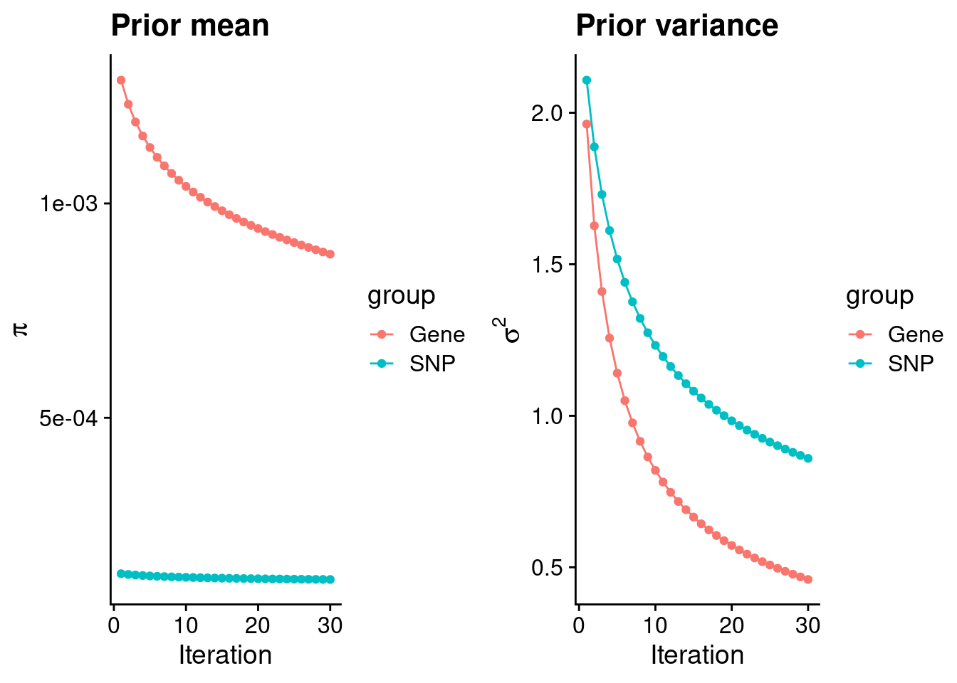
| Version | Author | Date |
|---|---|---|
| dfd2b5f | wesleycrouse | 2021-09-07 |
#estimated group prior
estimated_group_prior <- group_prior_rec[,ncol(group_prior_rec)]
names(estimated_group_prior) <- c("gene", "snp")
estimated_group_prior["snp"] <- estimated_group_prior["snp"]*thin #adjust parameter to account for thin argument
print(estimated_group_prior)
gene snp
0.0008817026 0.0001229032 #estimated group prior variance
estimated_group_prior_var <- group_prior_var_rec[,ncol(group_prior_var_rec)]
names(estimated_group_prior_var) <- c("gene", "snp")
print(estimated_group_prior_var) gene snp
0.4598246 0.8594798 #report sample size
print(sample_size)[1] 30565#report group size
group_size <- c(nrow(ctwas_gene_res), n_snps)
print(group_size)[1] 11095 8697330#estimated group PVE
estimated_group_pve <- estimated_group_prior_var*estimated_group_prior*group_size/sample_size #check PVE calculation
names(estimated_group_pve) <- c("gene", "snp")
print(estimated_group_pve) gene snp
0.0001471693 0.0300580291 #compare sum(PIP*mu2/sample_size) with above PVE calculation
c(sum(ctwas_gene_res$PVE),sum(ctwas_snp_res$PVE))[1] 0.003395404 0.652379670Genes with highest PIPs
#distribution of PIPs
hist(ctwas_gene_res$susie_pip, xlim=c(0,1), main="Distribution of Gene PIPs")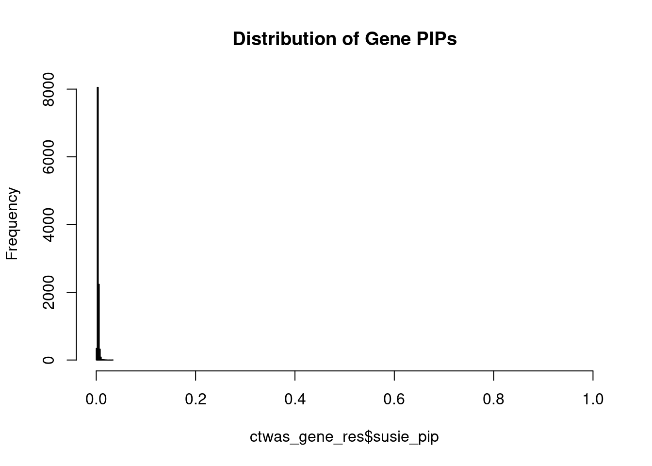
| Version | Author | Date |
|---|---|---|
| dfd2b5f | wesleycrouse | 2021-09-07 |
#genes with PIP>0.8 or 20 highest PIPs
head(ctwas_gene_res[order(-ctwas_gene_res$susie_pip),report_cols], max(sum(ctwas_gene_res$susie_pip>0.8), 20))
genename region_tag susie_pip mu2 PVE z
1760 RIOK3 18_12 0.033 8.44 9.0e-06 3.91
11151 IFI30 19_14 0.033 9.07 9.8e-06 4.62
1703 RSPO4 20_2 0.028 8.01 7.2e-06 3.67
375 TRIO 5_11 0.021 6.90 4.7e-06 3.29
8228 SPNS1 16_24 0.021 7.07 4.8e-06 3.46
3115 PLA2G4A 1_93 0.020 7.13 4.7e-06 3.66
4835 AOAH 7_27 0.020 7.01 4.6e-06 3.41
9221 ZNF552 19_39 0.019 6.78 4.1e-06 3.31
5730 ESPNL 2_141 0.018 6.49 3.8e-06 -3.29
6847 PDE9A 21_21 0.018 6.61 3.9e-06 -3.25
8575 GNG12 1_42 0.017 6.42 3.6e-06 -3.28
6193 CDC123 10_10 0.017 6.54 3.7e-06 3.24
1496 TCF20 22_18 0.017 6.33 3.6e-06 -3.13
3150 KMO 1_127 0.015 6.02 2.9e-06 -3.11
174 HHATL 3_31 0.015 6.13 3.1e-06 3.20
7342 ZDHHC19 3_120 0.015 6.03 3.0e-06 3.08
12226 RP11-326I11.4 4_119 0.015 5.82 2.8e-06 -2.95
9713 TMEM173 5_82 0.015 5.83 2.9e-06 -3.03
8960 JAKMIP2 5_86 0.015 6.05 3.0e-06 3.04
54 POLR2J 7_63 0.015 6.17 3.1e-06 3.20Genes with largest effect sizes
#plot PIP vs effect size
plot(ctwas_gene_res$susie_pip, ctwas_gene_res$mu2, xlab="PIP", ylab="mu^2", main="Gene PIPs vs Effect Size")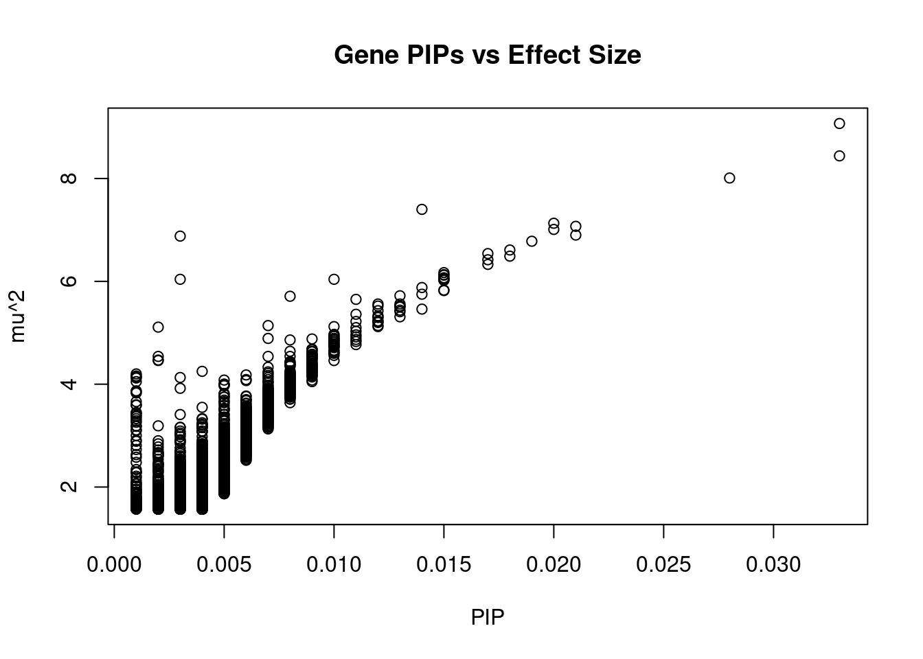
| Version | Author | Date |
|---|---|---|
| dfd2b5f | wesleycrouse | 2021-09-07 |
#genes with 20 largest effect sizes
head(ctwas_gene_res[order(-ctwas_gene_res$mu2),report_cols],20)
genename region_tag susie_pip mu2 PVE z
11151 IFI30 19_14 0.033 9.07 9.8e-06 4.62
1760 RIOK3 18_12 0.033 8.44 9.0e-06 3.91
1703 RSPO4 20_2 0.028 8.01 7.2e-06 3.67
9340 GAS1 9_45 0.014 7.40 3.3e-06 -3.55
3115 PLA2G4A 1_93 0.020 7.13 4.7e-06 3.66
8228 SPNS1 16_24 0.021 7.07 4.8e-06 3.46
4835 AOAH 7_27 0.020 7.01 4.6e-06 3.41
375 TRIO 5_11 0.021 6.90 4.7e-06 3.29
10855 HLA-G 6_26 0.003 6.88 7.8e-07 -3.39
9221 ZNF552 19_39 0.019 6.78 4.1e-06 3.31
6847 PDE9A 21_21 0.018 6.61 3.9e-06 -3.25
6193 CDC123 10_10 0.017 6.54 3.7e-06 3.24
5730 ESPNL 2_141 0.018 6.49 3.8e-06 -3.29
8575 GNG12 1_42 0.017 6.42 3.6e-06 -3.28
1496 TCF20 22_18 0.017 6.33 3.6e-06 -3.13
54 POLR2J 7_63 0.015 6.17 3.1e-06 3.20
174 HHATL 3_31 0.015 6.13 3.1e-06 3.20
8884 DOLK 9_66 0.015 6.12 3.0e-06 -3.07
6902 PCSK7 11_70 0.015 6.07 3.0e-06 -3.10
8960 JAKMIP2 5_86 0.015 6.05 3.0e-06 3.04Genes with highest PVE
#genes with 20 highest pve
head(ctwas_gene_res[order(-ctwas_gene_res$PVE),report_cols],20)
genename region_tag susie_pip mu2 PVE z
11151 IFI30 19_14 0.033 9.07 9.8e-06 4.62
1760 RIOK3 18_12 0.033 8.44 9.0e-06 3.91
1703 RSPO4 20_2 0.028 8.01 7.2e-06 3.67
8228 SPNS1 16_24 0.021 7.07 4.8e-06 3.46
3115 PLA2G4A 1_93 0.020 7.13 4.7e-06 3.66
375 TRIO 5_11 0.021 6.90 4.7e-06 3.29
4835 AOAH 7_27 0.020 7.01 4.6e-06 3.41
9221 ZNF552 19_39 0.019 6.78 4.1e-06 3.31
6847 PDE9A 21_21 0.018 6.61 3.9e-06 -3.25
5730 ESPNL 2_141 0.018 6.49 3.8e-06 -3.29
6193 CDC123 10_10 0.017 6.54 3.7e-06 3.24
8575 GNG12 1_42 0.017 6.42 3.6e-06 -3.28
1496 TCF20 22_18 0.017 6.33 3.6e-06 -3.13
9340 GAS1 9_45 0.014 7.40 3.3e-06 -3.55
174 HHATL 3_31 0.015 6.13 3.1e-06 3.20
54 POLR2J 7_63 0.015 6.17 3.1e-06 3.20
7342 ZDHHC19 3_120 0.015 6.03 3.0e-06 3.08
8960 JAKMIP2 5_86 0.015 6.05 3.0e-06 3.04
8884 DOLK 9_66 0.015 6.12 3.0e-06 -3.07
6902 PCSK7 11_70 0.015 6.07 3.0e-06 -3.10Genes with largest z scores
#genes with 20 largest z scores
head(ctwas_gene_res[order(-abs(ctwas_gene_res$z)),report_cols],20)
genename region_tag susie_pip mu2 PVE z
11151 IFI30 19_14 0.033 9.07 9.8e-06 4.62
1760 RIOK3 18_12 0.033 8.44 9.0e-06 3.91
1703 RSPO4 20_2 0.028 8.01 7.2e-06 3.67
3115 PLA2G4A 1_93 0.020 7.13 4.7e-06 3.66
9340 GAS1 9_45 0.014 7.40 3.3e-06 -3.55
8228 SPNS1 16_24 0.021 7.07 4.8e-06 3.46
4835 AOAH 7_27 0.020 7.01 4.6e-06 3.41
10855 HLA-G 6_26 0.003 6.88 7.8e-07 -3.39
8241 RAC3 17_46 0.011 5.22 1.9e-06 3.32
9221 ZNF552 19_39 0.019 6.78 4.1e-06 3.31
5730 ESPNL 2_141 0.018 6.49 3.8e-06 -3.29
375 TRIO 5_11 0.021 6.90 4.7e-06 3.29
8575 GNG12 1_42 0.017 6.42 3.6e-06 -3.28
10735 FAM229B 6_75 0.012 5.43 2.1e-06 3.27
6847 PDE9A 21_21 0.018 6.61 3.9e-06 -3.25
6193 CDC123 10_10 0.017 6.54 3.7e-06 3.24
174 HHATL 3_31 0.015 6.13 3.1e-06 3.20
54 POLR2J 7_63 0.015 6.17 3.1e-06 3.20
6534 N6AMT1 21_11 0.013 5.72 2.5e-06 3.18
12299 U91328.19 6_20 0.009 4.68 1.4e-06 3.13Comparing z scores and PIPs
#set nominal signifiance threshold for z scores
alpha <- 0.05

#bonferroni adjusted threshold for z scores
sig_thresh <- qnorm(1-(alpha/nrow(ctwas_gene_res)/2), lower=T)

#Q-Q plot for z scores
obs_z <- ctwas_gene_res$z[order(ctwas_gene_res$z)]
exp_z <- qnorm((1:nrow(ctwas_gene_res))/nrow(ctwas_gene_res))

plot(exp_z, obs_z, xlab="Expected z", ylab="Observed z", main="Gene z score Q-Q plot")
abline(a=0,b=1)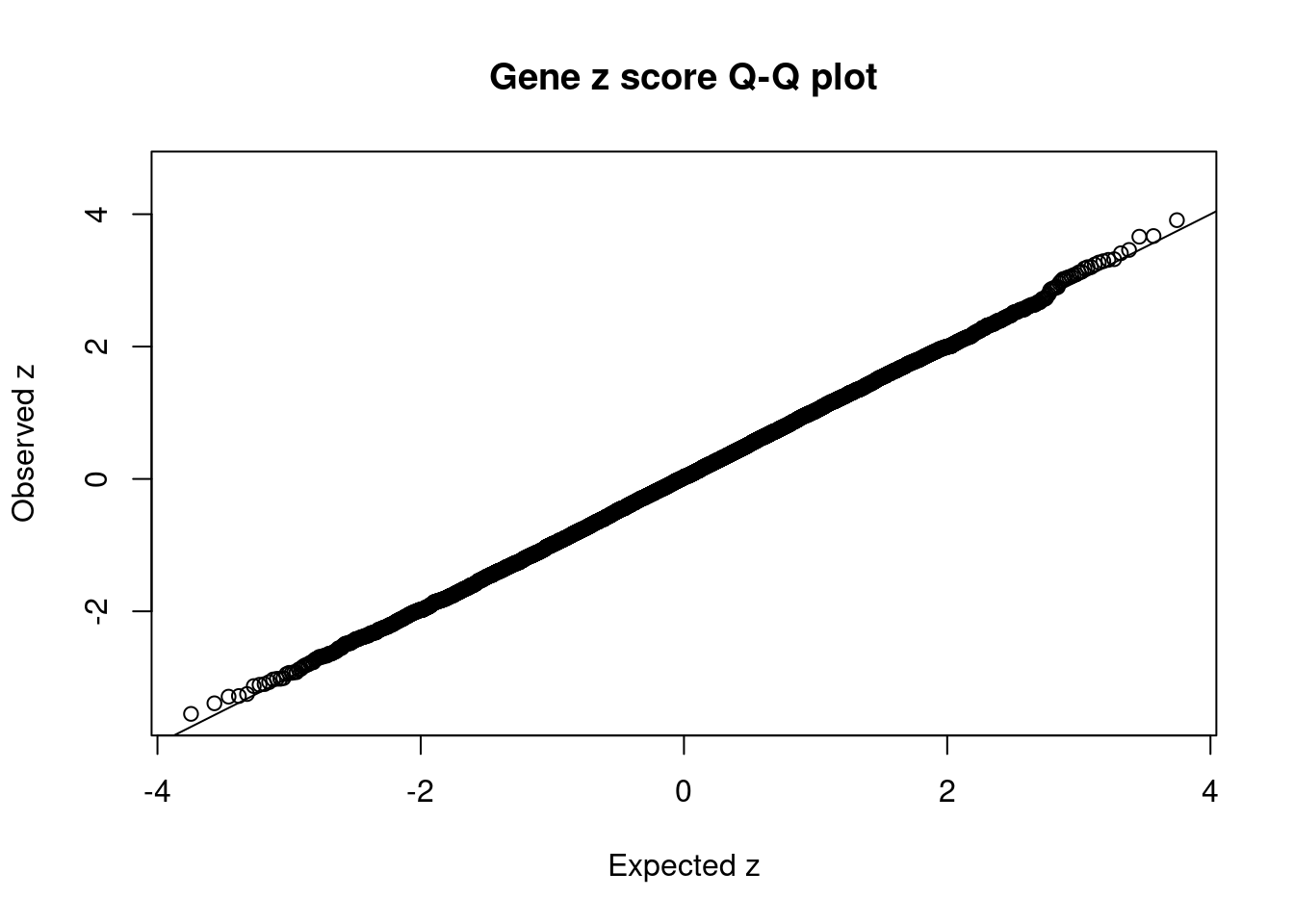
| Version | Author | Date |
|---|---|---|
| dfd2b5f | wesleycrouse | 2021-09-07 |
#plot z score vs PIP
plot(abs(ctwas_gene_res$z), ctwas_gene_res$susie_pip, xlab="abs(z)", ylab="PIP")
abline(v=sig_thresh, col="red", lty=2)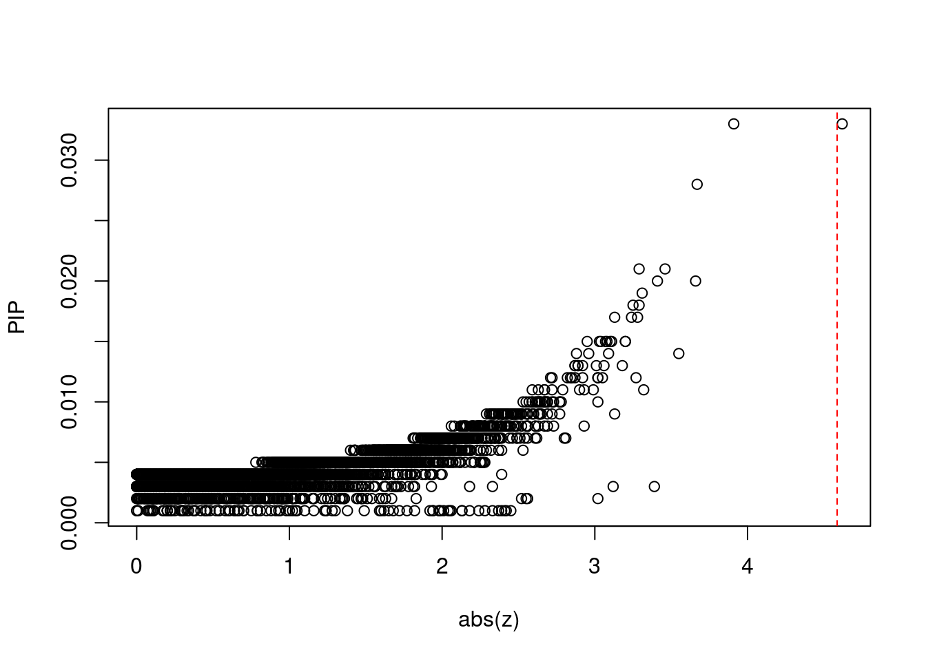
| Version | Author | Date |
|---|---|---|
| dfd2b5f | wesleycrouse | 2021-09-07 |
#proportion of significant z scores
mean(abs(ctwas_gene_res$z) > sig_thresh)
[1] 9.013069e-05#genes with most significant z scores
head(ctwas_gene_res[order(-abs(ctwas_gene_res$z)),report_cols],20) genename region_tag susie_pip mu2 PVE z
11151 IFI30 19_14 0.033 9.07 9.8e-06 4.62
1760 RIOK3 18_12 0.033 8.44 9.0e-06 3.91
1703 RSPO4 20_2 0.028 8.01 7.2e-06 3.67
3115 PLA2G4A 1_93 0.020 7.13 4.7e-06 3.66
9340 GAS1 9_45 0.014 7.40 3.3e-06 -3.55
8228 SPNS1 16_24 0.021 7.07 4.8e-06 3.46
4835 AOAH 7_27 0.020 7.01 4.6e-06 3.41
10855 HLA-G 6_26 0.003 6.88 7.8e-07 -3.39
8241 RAC3 17_46 0.011 5.22 1.9e-06 3.32
9221 ZNF552 19_39 0.019 6.78 4.1e-06 3.31
5730 ESPNL 2_141 0.018 6.49 3.8e-06 -3.29
375 TRIO 5_11 0.021 6.90 4.7e-06 3.29
8575 GNG12 1_42 0.017 6.42 3.6e-06 -3.28
10735 FAM229B 6_75 0.012 5.43 2.1e-06 3.27
6847 PDE9A 21_21 0.018 6.61 3.9e-06 -3.25
6193 CDC123 10_10 0.017 6.54 3.7e-06 3.24
174 HHATL 3_31 0.015 6.13 3.1e-06 3.20
54 POLR2J 7_63 0.015 6.17 3.1e-06 3.20
6534 N6AMT1 21_11 0.013 5.72 2.5e-06 3.18
12299 U91328.19 6_20 0.009 4.68 1.4e-06 3.13Locus plots for genes and SNPs
ctwas_gene_res_sortz <- ctwas_gene_res[order(-abs(ctwas_gene_res$z)),]

n_plots <- 5
for (region_tag_plot in head(unique(ctwas_gene_res_sortz$region_tag), n_plots)){
  ctwas_res_region <-  ctwas_res[ctwas_res$region_tag==region_tag_plot,]
  start <- min(ctwas_res_region$pos)
  end <- max(ctwas_res_region$pos)

  ctwas_res_region <- ctwas_res_region[order(ctwas_res_region$pos),]
  ctwas_res_region_gene <- ctwas_res_region[ctwas_res_region$type=="gene",]
  ctwas_res_region_snp <- ctwas_res_region[ctwas_res_region$type=="SNP",]

  #region name
  print(paste0("Region: ", region_tag_plot))

  #table of genes in region
  print(ctwas_res_region_gene[,report_cols])

  par(mfrow=c(4,1))

  #gene z scores
  plot(ctwas_res_region_gene$pos, abs(ctwas_res_region_gene$z), xlab="Position", ylab="abs(gene_z)", xlim=c(start,end),
   ylim=c(0,max(sig_thresh, abs(ctwas_res_region_gene$z))),
   main=paste0("Region: ", region_tag_plot))
  abline(h=sig_thresh,col="red",lty=2)

  #significance threshold for SNPs
  alpha_snp <- 5*10^(-8)
  sig_thresh_snp <- qnorm(1-alpha_snp/2, lower=T)

  #snp z scores
  plot(ctwas_res_region_snp$pos, abs(ctwas_res_region_snp$z), xlab="Position", ylab="abs(snp_z)",xlim=c(start,end),
   ylim=c(0,max(sig_thresh_snp, max(abs(ctwas_res_region_snp$z)))))
  abline(h=sig_thresh_snp,col="purple",lty=2)

  #gene pips
  plot(ctwas_res_region_gene$pos, ctwas_res_region_gene$susie_pip, xlab="Position", ylab="Gene PIP", xlim=c(start,end), ylim=c(0,1))
  abline(h=0.8,col="blue",lty=2)

  #snp pips
  plot(ctwas_res_region_snp$pos, ctwas_res_region_snp$susie_pip, xlab="Position", ylab="SNP PIP", xlim=c(start,end), ylim=c(0,1))
  abline(h=0.8,col="blue",lty=2)
}
[1] "Region: 19_14"
genename region_tag susie_pip mu2 PVE z
3962 KLF2 19_14 0.004 2.07 2.5e-07 -1.02
2018 C19orf44 19_14 0.003 1.58 1.6e-07 -0.14
1117 CHERP 19_14 0.003 1.70 1.8e-07 -0.54
12174 CTD-3222D19.12 19_14 0.003 1.59 1.6e-07 0.22
3960 SLC35E1 19_14 0.004 1.97 2.3e-07 -0.89
12158 CTC-429P9.2 19_14 0.003 1.78 1.9e-07 -0.65
2019 MED26 19_14 0.003 1.58 1.6e-07 0.07
11080 SMIM7 19_14 0.008 4.42 1.1e-06 2.47
818 TMEM38A 19_14 0.006 3.68 7.3e-07 -2.10
3959 SIN3B 19_14 0.003 1.61 1.7e-07 -0.29
3963 F2RL3 19_14 0.004 2.26 2.8e-07 1.19
6836 CPAMD8 19_14 0.003 1.58 1.6e-07 -0.14
4284 HAUS8 19_14 0.003 1.93 2.2e-07 0.84
1408 MYO9B 19_14 0.004 2.43 3.2e-07 -1.35
471 USE1 19_14 0.004 2.55 3.5e-07 -1.44
1407 OCEL1 19_14 0.004 2.64 3.8e-07 1.54
6837 NR2F6 19_14 0.009 4.88 1.4e-06 2.64
2071 BABAM1 19_14 0.008 4.64 1.2e-06 2.61
6838 ANKLE1 19_14 0.004 2.19 2.7e-07 -1.20
4174 DDA1 19_14 0.008 4.44 1.1e-06 -2.56
3940 ABHD8 19_14 0.004 2.19 2.7e-07 1.18
4169 GTPBP3 19_14 0.003 1.70 1.8e-07 -0.52
863 ANO8 19_14 0.003 1.67 1.7e-07 -0.44
12603 BISPR 19_14 0.003 1.63 1.7e-07 0.35
5480 MVB12A 19_14 0.003 1.58 1.6e-07 0.02
10065 TMEM221 19_14 0.003 1.95 2.2e-07 -0.89
4171 SLC27A1 19_14 0.003 1.76 1.9e-07 -0.64
4176 PGLS 19_14 0.006 3.55 6.7e-07 1.99
7903 FAM129C 19_14 0.003 1.62 1.7e-07 -0.30
4173 COLGALT1 19_14 0.003 1.72 1.8e-07 -0.56
4192 MAP1S 19_14 0.003 1.72 1.8e-07 0.55
4191 FCHO1 19_14 0.004 2.12 2.6e-07 1.08
11691 INSL3 19_14 0.003 1.67 1.7e-07 0.46
2110 RPL18A 19_14 0.004 2.37 3.1e-07 -1.30
112 CCDC124 19_14 0.005 2.91 4.5e-07 -1.66
1392 IL12RB1 19_14 0.005 2.80 4.2e-07 -1.69
1405 MAST3 19_14 0.004 2.65 3.8e-07 1.94
11151 IFI30 19_14 0.033 9.07 9.8e-06 4.62
11815 MPV17L2 19_14 0.003 1.63 1.7e-07 -0.35
2111 RAB3A 19_14 0.005 2.80 4.2e-07 1.61
4198 KIAA1683 19_14 0.004 2.16 2.6e-07 -0.98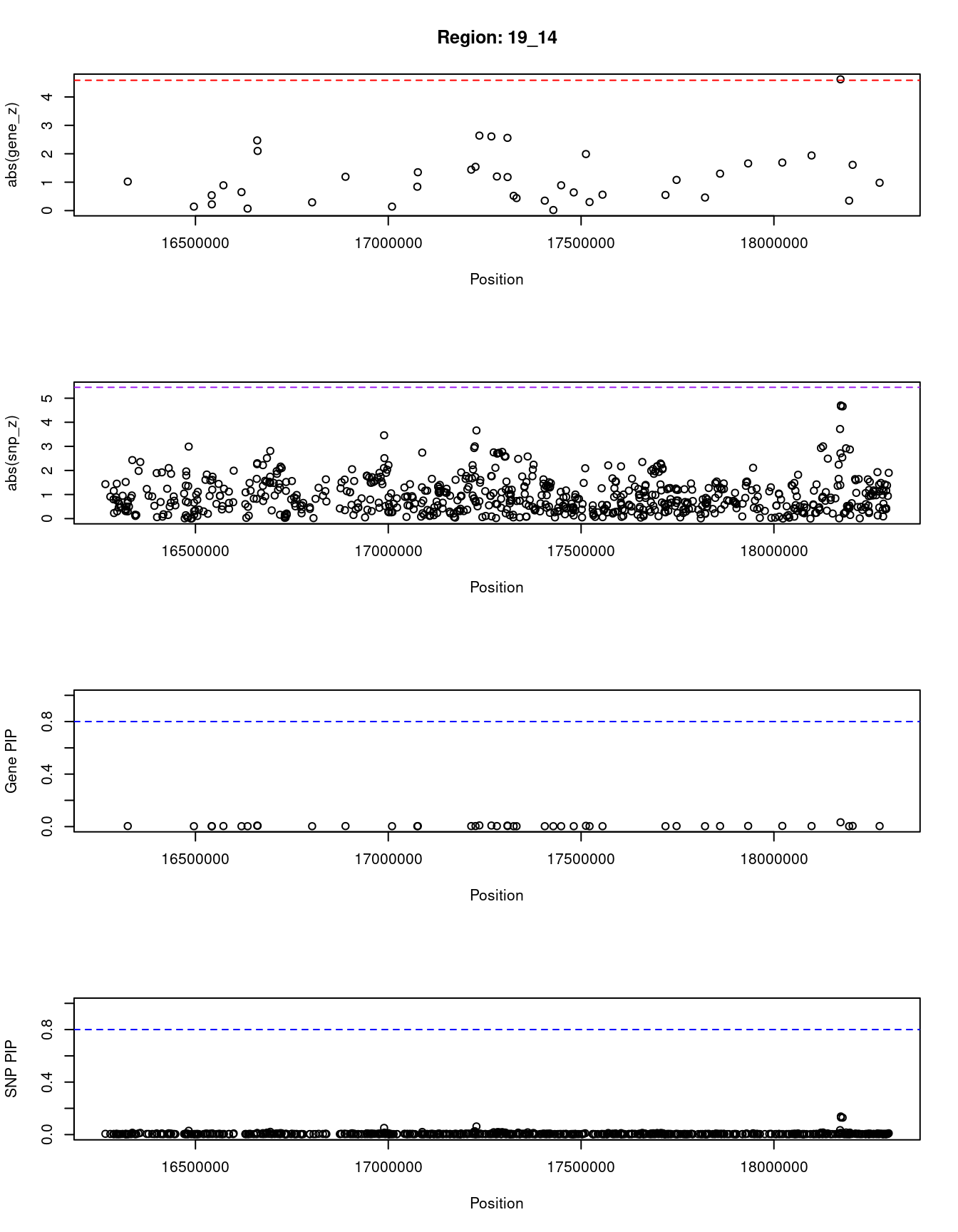
| Version | Author | Date |
|---|---|---|
| dfd2b5f | wesleycrouse | 2021-09-07 |
[1] "Region: 18_12"
           genename region_tag susie_pip  mu2     PVE     z
4603        CABLES1      18_12     0.004 1.58 1.9e-07 -0.04
4602        TMEM241      18_12     0.004 2.07 3.0e-07  1.02
1760          RIOK3      18_12     0.033 8.44 9.0e-06  3.91
5420        C18orf8      18_12     0.004 1.58 1.9e-07  0.15
5421           NPC1      18_12     0.004 1.71 2.2e-07  0.56
8044         TTC39C      18_12     0.005 2.37 3.7e-07 -1.29
6386          CABYR      18_12     0.004 1.86 2.5e-07 -0.78
5418        OSBPL1A      18_12     0.005 2.31 3.6e-07  1.21
6387         IMPACT      18_12     0.004 1.59 2.0e-07  0.21
4601           HRH4      18_12     0.004 1.99 2.8e-07  0.95
12088 RP11-178F10.2      18_12     0.004 2.00 2.8e-07  0.96
10663        ZNF521      18_12     0.004 1.87 2.5e-07 -0.78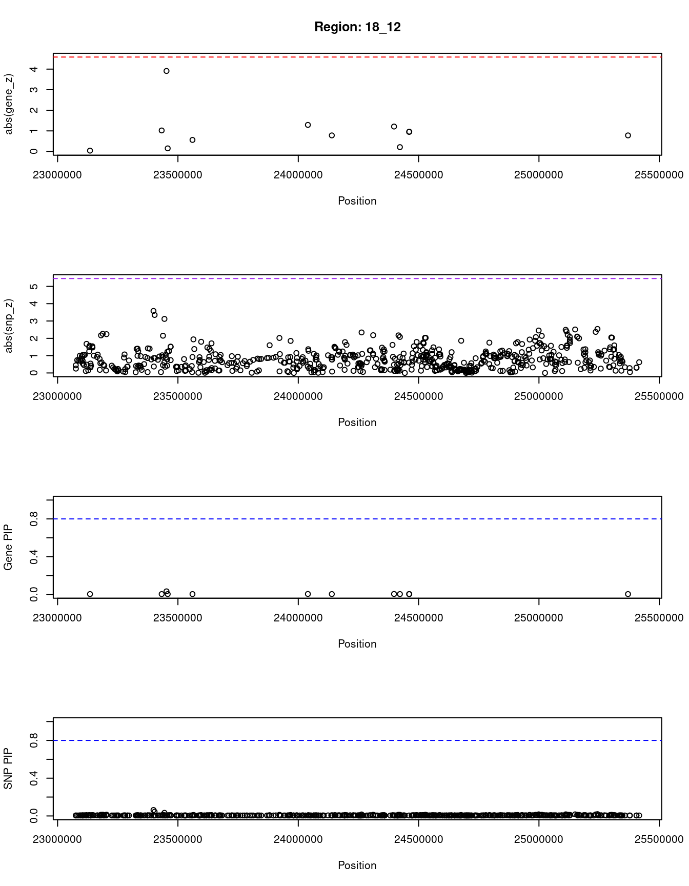
| Version | Author | Date |
|---|---|---|
| dfd2b5f | wesleycrouse | 2021-09-07 |
[1] "Region: 20_2"
       genename region_tag susie_pip  mu2     PVE     z
3860    FAM110A       20_2     0.005 2.90 5.2e-07  1.66
1703      RSPO4       20_2     0.028 8.01 7.2e-06  3.67
3841      PSMF1       20_2     0.004 1.74 2.2e-07  0.62
11141 C20orf202       20_2     0.004 1.60 1.9e-07  0.22
1706       SNPH       20_2     0.006 2.98 5.5e-07  1.70
3834     SDCBP2       20_2     0.005 2.62 4.3e-07 -1.47
1195     FKBP1A       20_2     0.004 1.60 1.9e-07  0.22
1196     NSFL1C       20_2     0.004 1.80 2.3e-07 -0.70
10226    SIRPB2       20_2     0.004 1.60 1.9e-07 -0.21
3861      SIRPD       20_2     0.004 1.64 2.0e-07 -0.38
1708     SIRPB1       20_2     0.004 1.61 1.9e-07  0.29
1209      SIRPG       20_2     0.004 1.61 1.9e-07  0.25
10538     SIRPA       20_2     0.004 1.61 1.9e-07  0.28
3845      STK35       20_2     0.004 1.79 2.3e-07  0.67
3836       TGM3       20_2     0.005 2.30 3.4e-07 -1.23
3846      SNRPB       20_2     0.005 2.76 4.7e-07  1.56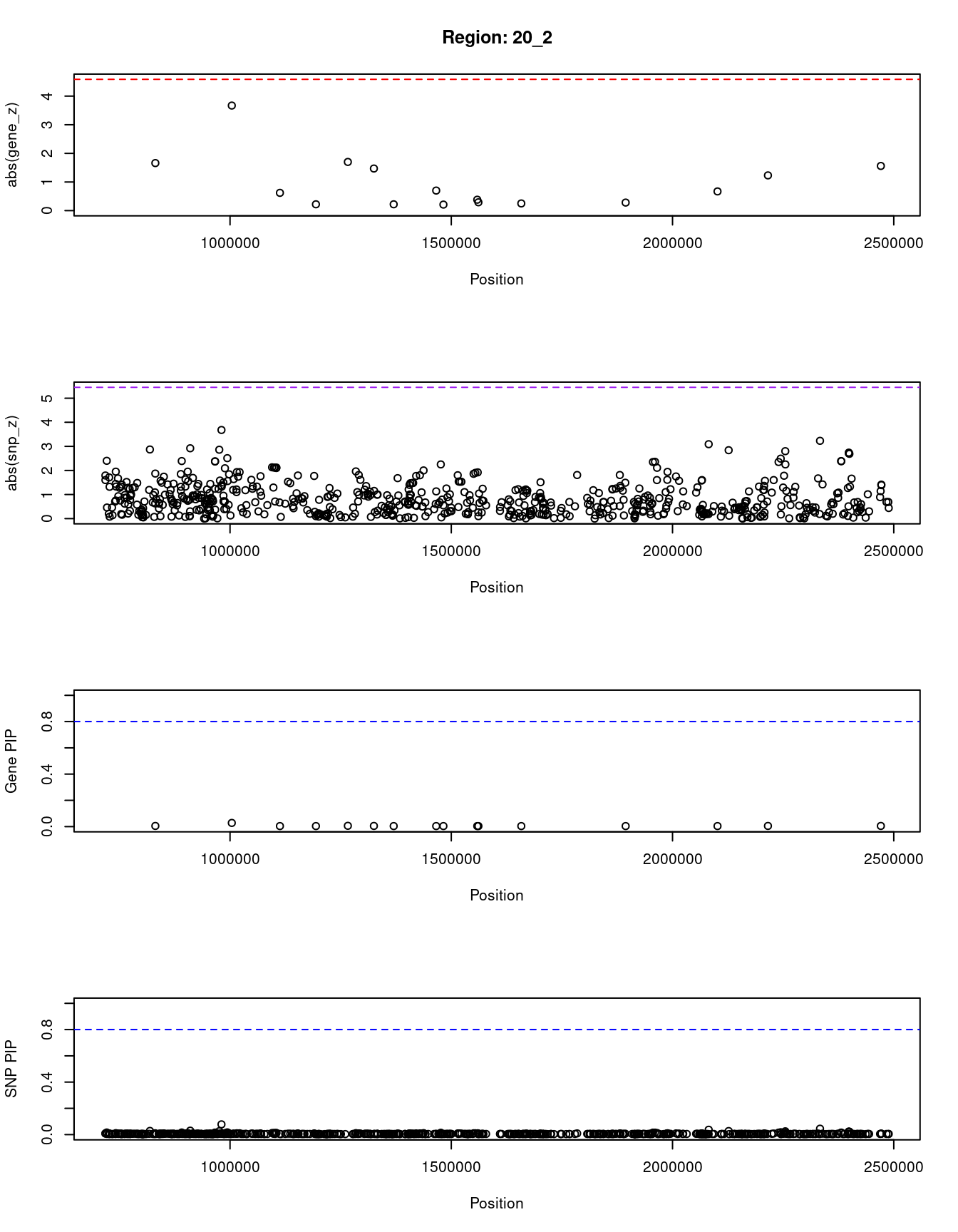
| Version | Author | Date |
|---|---|---|
| dfd2b5f | wesleycrouse | 2021-09-07 |
[1] "Region: 1_93"
     genename region_tag susie_pip  mu2     PVE    z
3115  PLA2G4A       1_93      0.02 7.13 4.7e-06 3.66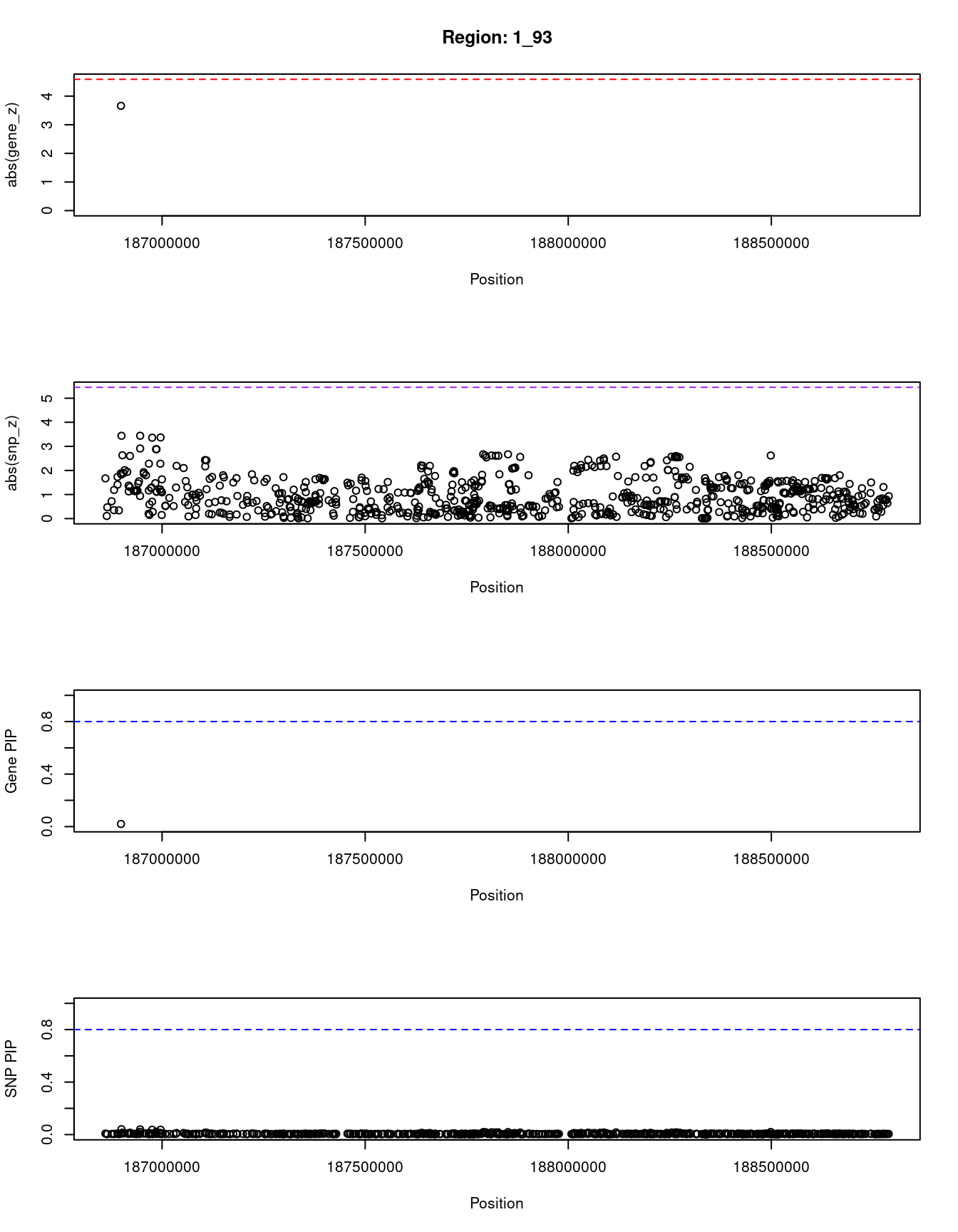
| Version | Author | Date |
|---|---|---|
| dfd2b5f | wesleycrouse | 2021-09-07 |
[1] "Region: 9_45"
      genename region_tag susie_pip  mu2     PVE     z
4666     GOLM1       9_45     0.002 1.69 1.2e-07  0.49
4669     ISCA1       9_45     0.002 1.68 1.2e-07  0.47
1053    ZCCHC6       9_45     0.002 1.69 1.2e-07 -0.49
9340      GAS1       9_45     0.014 7.40 3.3e-06 -3.55
10324    DAPK1       9_45     0.002 1.58 1.1e-07 -0.11
4664      CTSL       9_45     0.003 2.53 2.4e-07 -1.39
2245     SPIN1       9_45     0.003 2.46 2.3e-07 -1.39
4147     NXNL2       9_45     0.002 1.58 1.1e-07 -0.11
3659      CKS2       9_45     0.002 1.58 1.1e-07 -0.05
10033 SECISBP2       9_45     0.003 2.50 2.4e-07  1.41
10035   SEMA4D       9_45     0.002 1.58 1.1e-07 -0.07
4163   GADD45G       9_45     0.003 2.40 2.2e-07 -1.29
11484  UNQ6494       9_45     0.002 1.61 1.2e-07  0.26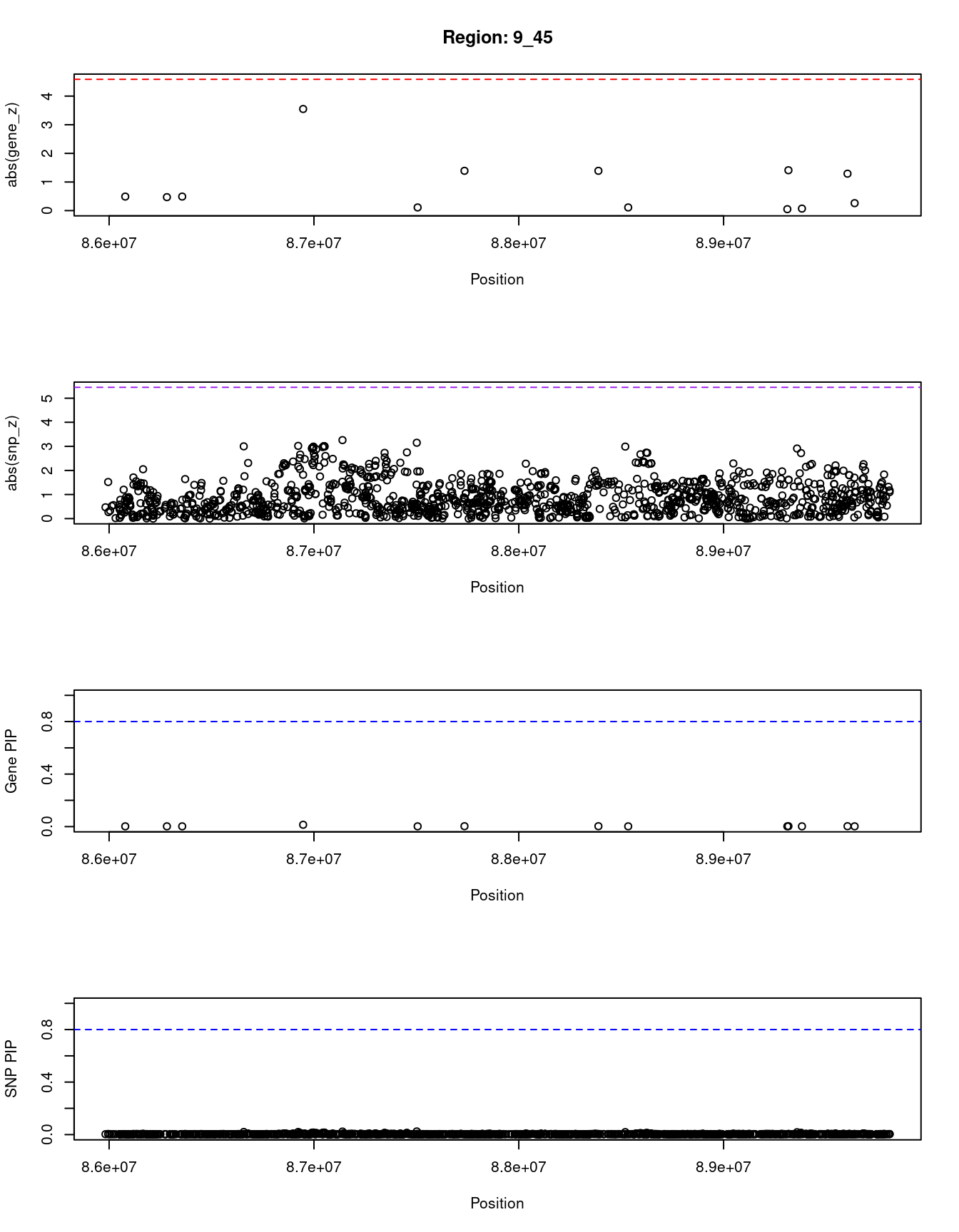
| Version | Author | Date |
|---|---|---|
| dfd2b5f | wesleycrouse | 2021-09-07 |
SNPs with highest PIPs
#snps with PIP>0.8 or 20 highest PIPs
head(ctwas_snp_res[order(-ctwas_snp_res$susie_pip),report_cols_snps],
max(sum(ctwas_snp_res$susie_pip>0.8), 20))
id region_tag susie_pip mu2 PVE z
832971 rs11557577 20_13 0.240 21.22 1.7e-04 -4.76
221280 rs117111501 4_41 0.224 21.81 1.6e-04 4.73
838805 rs6017234 20_27 0.214 20.86 1.5e-04 -4.60
242736 rs7660796 4_80 0.168 19.45 1.1e-04 4.38
505868 rs75155685 9_51 0.165 19.62 1.1e-04 4.68
607479 rs10772815 12_7 0.150 18.79 9.2e-05 -4.27
608967 rs56198451 12_11 0.141 18.70 8.6e-05 4.45
813014 rs273265 19_14 0.138 19.15 8.6e-05 -4.70
188130 rs190072323 3_97 0.137 18.33 8.2e-05 4.08
208954 rs35945249 4_18 0.137 18.22 8.2e-05 -4.23
780163 rs1675273 17_44 0.134 18.50 8.1e-05 4.21
650317 rs562115589 13_7 0.133 18.39 8.0e-05 -4.20
813015 rs2241089 19_14 0.130 18.87 8.0e-05 -4.67
3511 rs79089220 1_9 0.129 18.07 7.7e-05 4.08
521053 rs17144212 10_8 0.129 18.15 7.6e-05 -4.14
813017 rs4808757 19_14 0.129 18.83 8.0e-05 -4.66
12749 rs116039993 1_27 0.127 17.93 7.5e-05 4.03
505859 rs118013517 9_51 0.125 18.25 7.5e-05 4.52
856603 rs553932 21_22 0.123 17.98 7.3e-05 -4.33
527922 rs117340939 10_20 0.121 18.51 7.3e-05 -4.13SNPs with largest effect sizes
#plot PIP vs effect size
plot(ctwas_snp_res$susie_pip, ctwas_snp_res$mu2, xlab="PIP", ylab="mu^2", main="SNP PIPs vs Effect Size")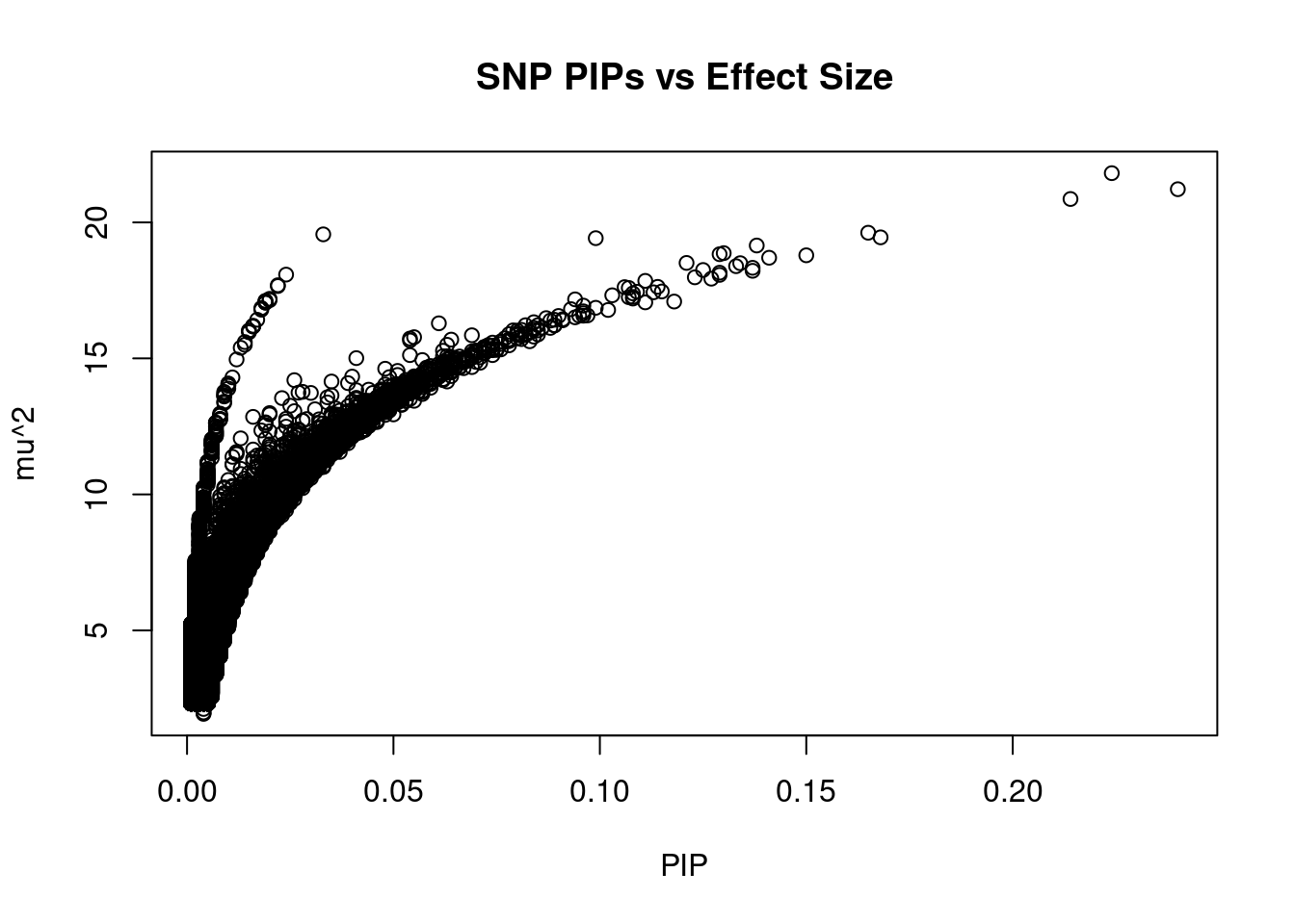
| Version | Author | Date |
|---|---|---|
| dfd2b5f | wesleycrouse | 2021-09-07 |
#SNPs with 50 largest effect sizes
head(ctwas_snp_res[order(-ctwas_snp_res$mu2),report_cols_snps],50)
id region_tag susie_pip mu2 PVE z
221280 rs117111501 4_41 0.224 21.81 1.6e-04 4.73
832971 rs11557577 20_13 0.240 21.22 1.7e-04 -4.76
838805 rs6017234 20_27 0.214 20.86 1.5e-04 -4.60
505868 rs75155685 9_51 0.165 19.62 1.1e-04 4.68
334851 rs74434374 6_26 0.033 19.56 2.1e-05 -4.37
242736 rs7660796 4_80 0.168 19.45 1.1e-04 4.38
824212 rs1966573 19_37 0.099 19.42 6.3e-05 -4.20
813014 rs273265 19_14 0.138 19.15 8.6e-05 -4.70
813015 rs2241089 19_14 0.130 18.87 8.0e-05 -4.67
813017 rs4808757 19_14 0.129 18.83 8.0e-05 -4.66
607479 rs10772815 12_7 0.150 18.79 9.2e-05 -4.27
608967 rs56198451 12_11 0.141 18.70 8.6e-05 4.45
527922 rs117340939 10_20 0.121 18.51 7.3e-05 -4.13
780163 rs1675273 17_44 0.134 18.50 8.1e-05 4.21
650317 rs562115589 13_7 0.133 18.39 8.0e-05 -4.20
188130 rs190072323 3_97 0.137 18.33 8.2e-05 4.08
505859 rs118013517 9_51 0.125 18.25 7.5e-05 4.52
208954 rs35945249 4_18 0.137 18.22 8.2e-05 -4.23
521053 rs17144212 10_8 0.129 18.15 7.6e-05 -4.14
334909 rs79594290 6_26 0.024 18.08 1.4e-05 -4.08
3511 rs79089220 1_9 0.129 18.07 7.7e-05 4.08
856603 rs553932 21_22 0.123 17.98 7.3e-05 -4.33
12749 rs116039993 1_27 0.127 17.93 7.5e-05 4.03
97634 rs200418470 2_58 0.111 17.85 6.5e-05 4.19
335654 rs183736834 6_26 0.022 17.69 1.3e-05 -4.29
335693 rs35686990 6_26 0.022 17.66 1.3e-05 -4.29
608971 rs16907395 12_11 0.114 17.63 6.6e-05 4.31
97636 rs76082620 2_58 0.106 17.62 6.1e-05 4.16
160726 rs9311895 3_43 0.107 17.59 6.2e-05 -3.97
704311 rs77066728 14_50 0.115 17.46 6.6e-05 3.99
297670 rs115431743 5_62 0.109 17.45 6.2e-05 -4.10
709342 rs117521738 15_5 0.113 17.43 6.4e-05 -3.98
297679 rs116673434 5_62 0.108 17.39 6.1e-05 -4.10
380830 rs12198594 6_112 0.103 17.32 5.8e-05 3.99
367943 rs34181568 6_88 0.108 17.26 6.1e-05 -3.90
520762 rs484392 10_8 0.107 17.25 6.0e-05 3.92
801441 rs8084578 18_38 0.108 17.20 6.1e-05 -4.01
335619 rs192408808 6_26 0.020 17.19 1.1e-05 -4.23
510103 rs10981735 9_58 0.094 17.17 5.3e-05 4.11
334896 rs61740337 6_26 0.020 17.14 1.1e-05 -3.94
334024 rs73728438 6_26 0.019 17.11 1.1e-05 -3.88
334025 rs7762578 6_26 0.019 17.11 1.1e-05 -3.88
814319 rs78119665 19_17 0.118 17.09 6.6e-05 -4.04
1530 rs12082538 1_4 0.111 17.06 6.2e-05 -3.92
335526 rs73730378 6_26 0.019 17.05 1.1e-05 -4.22
335625 rs76434237 6_26 0.019 17.05 1.1e-05 -4.22
627833 rs150360326 12_46 0.096 16.94 5.3e-05 -3.87
735252 rs3785217 16_8 0.099 16.86 5.5e-05 3.90
335620 rs536856134 6_26 0.018 16.85 1.0e-05 -4.19
175280 rs9867405 3_71 0.093 16.81 5.1e-05 4.13SNPs with highest PVE
#SNPs with 50 highest pve
head(ctwas_snp_res[order(-ctwas_snp_res$PVE),report_cols_snps],50)
id region_tag susie_pip mu2 PVE z
832971 rs11557577 20_13 0.240 21.22 1.7e-04 -4.76
221280 rs117111501 4_41 0.224 21.81 1.6e-04 4.73
838805 rs6017234 20_27 0.214 20.86 1.5e-04 -4.60
242736 rs7660796 4_80 0.168 19.45 1.1e-04 4.38
505868 rs75155685 9_51 0.165 19.62 1.1e-04 4.68
607479 rs10772815 12_7 0.150 18.79 9.2e-05 -4.27
608967 rs56198451 12_11 0.141 18.70 8.6e-05 4.45
813014 rs273265 19_14 0.138 19.15 8.6e-05 -4.70
188130 rs190072323 3_97 0.137 18.33 8.2e-05 4.08
208954 rs35945249 4_18 0.137 18.22 8.2e-05 -4.23
780163 rs1675273 17_44 0.134 18.50 8.1e-05 4.21
650317 rs562115589 13_7 0.133 18.39 8.0e-05 -4.20
813015 rs2241089 19_14 0.130 18.87 8.0e-05 -4.67
813017 rs4808757 19_14 0.129 18.83 8.0e-05 -4.66
3511 rs79089220 1_9 0.129 18.07 7.7e-05 4.08
521053 rs17144212 10_8 0.129 18.15 7.6e-05 -4.14
12749 rs116039993 1_27 0.127 17.93 7.5e-05 4.03
505859 rs118013517 9_51 0.125 18.25 7.5e-05 4.52
527922 rs117340939 10_20 0.121 18.51 7.3e-05 -4.13
856603 rs553932 21_22 0.123 17.98 7.3e-05 -4.33
608971 rs16907395 12_11 0.114 17.63 6.6e-05 4.31
704311 rs77066728 14_50 0.115 17.46 6.6e-05 3.99
814319 rs78119665 19_17 0.118 17.09 6.6e-05 -4.04
97634 rs200418470 2_58 0.111 17.85 6.5e-05 4.19
709342 rs117521738 15_5 0.113 17.43 6.4e-05 -3.98
824212 rs1966573 19_37 0.099 19.42 6.3e-05 -4.20
1530 rs12082538 1_4 0.111 17.06 6.2e-05 -3.92
160726 rs9311895 3_43 0.107 17.59 6.2e-05 -3.97
297670 rs115431743 5_62 0.109 17.45 6.2e-05 -4.10
97636 rs76082620 2_58 0.106 17.62 6.1e-05 4.16
297679 rs116673434 5_62 0.108 17.39 6.1e-05 -4.10
367943 rs34181568 6_88 0.108 17.26 6.1e-05 -3.90
801441 rs8084578 18_38 0.108 17.20 6.1e-05 -4.01
520762 rs484392 10_8 0.107 17.25 6.0e-05 3.92
380830 rs12198594 6_112 0.103 17.32 5.8e-05 3.99
262078 rs28684807 4_117 0.102 16.78 5.6e-05 3.83
735252 rs3785217 16_8 0.099 16.86 5.5e-05 3.90
52775 rs17187009 1_105 0.097 16.58 5.3e-05 3.81
414896 rs1734886 7_63 0.096 16.73 5.3e-05 4.11
510103 rs10981735 9_58 0.094 17.17 5.3e-05 4.11
627833 rs150360326 12_46 0.096 16.94 5.3e-05 -3.87
166197 rs12636636 3_54 0.096 16.66 5.2e-05 3.98
289169 rs56203338 5_45 0.096 16.57 5.2e-05 -3.88
675062 rs150602177 13_53 0.095 16.57 5.2e-05 -3.84
119153 rs77191462 2_105 0.094 16.51 5.1e-05 -3.78
175280 rs9867405 3_71 0.093 16.81 5.1e-05 4.13
57714 rs74751225 1_114 0.090 16.56 4.9e-05 3.82
645383 rs264505 12_79 0.091 16.44 4.9e-05 3.80
693111 rs11622348 14_28 0.091 16.40 4.9e-05 3.78
781250 rs9890434 17_46 0.089 16.42 4.8e-05 4.41SNPs with largest z scores
#SNPs with 50 largest z scores
head(ctwas_snp_res[order(-abs(ctwas_snp_res$z)),report_cols_snps],50)
id region_tag susie_pip mu2 PVE z
832971 rs11557577 20_13 0.240 21.22 1.7e-04 -4.76
221280 rs117111501 4_41 0.224 21.81 1.6e-04 4.73
813014 rs273265 19_14 0.138 19.15 8.6e-05 -4.70
505868 rs75155685 9_51 0.165 19.62 1.1e-04 4.68
813015 rs2241089 19_14 0.130 18.87 8.0e-05 -4.67
813017 rs4808757 19_14 0.129 18.83 8.0e-05 -4.66
838805 rs6017234 20_27 0.214 20.86 1.5e-04 -4.60
505859 rs118013517 9_51 0.125 18.25 7.5e-05 4.52
608967 rs56198451 12_11 0.141 18.70 8.6e-05 4.45
781250 rs9890434 17_46 0.089 16.42 4.8e-05 4.41
242736 rs7660796 4_80 0.168 19.45 1.1e-04 4.38
781249 rs74002714 17_46 0.085 16.22 4.5e-05 4.38
334851 rs74434374 6_26 0.033 19.56 2.1e-05 -4.37
781247 rs74002712 17_46 0.080 15.93 4.2e-05 4.34
856603 rs553932 21_22 0.123 17.98 7.3e-05 -4.33
781243 rs9912120 17_46 0.077 15.74 4.0e-05 4.32
608971 rs16907395 12_11 0.114 17.63 6.6e-05 4.31
335654 rs183736834 6_26 0.022 17.69 1.3e-05 -4.29
335693 rs35686990 6_26 0.022 17.66 1.3e-05 -4.29
781244 rs74002710 17_46 0.073 15.47 3.7e-05 4.28
607479 rs10772815 12_7 0.150 18.79 9.2e-05 -4.27
781238 rs112313398 17_46 0.072 15.42 3.6e-05 4.27
208954 rs35945249 4_18 0.137 18.22 8.2e-05 -4.23
335619 rs192408808 6_26 0.020 17.19 1.1e-05 -4.23
781245 rs112225092 17_46 0.072 15.40 3.6e-05 4.23
335526 rs73730378 6_26 0.019 17.05 1.1e-05 -4.22
335625 rs76434237 6_26 0.019 17.05 1.1e-05 -4.22
780163 rs1675273 17_44 0.134 18.50 8.1e-05 4.21
650317 rs562115589 13_7 0.133 18.39 8.0e-05 -4.20
824212 rs1966573 19_37 0.099 19.42 6.3e-05 -4.20
97634 rs200418470 2_58 0.111 17.85 6.5e-05 4.19
335620 rs536856134 6_26 0.018 16.85 1.0e-05 -4.19
335511 rs199640993 6_26 0.018 16.79 9.9e-06 -4.18
97636 rs76082620 2_58 0.106 17.62 6.1e-05 4.16
608965 rs147901559 12_11 0.088 16.39 4.7e-05 4.16
521053 rs17144212 10_8 0.129 18.15 7.6e-05 -4.14
175280 rs9867405 3_71 0.093 16.81 5.1e-05 4.13
527922 rs117340939 10_20 0.121 18.51 7.3e-05 -4.13
335277 rs9469134 6_26 0.016 16.20 8.4e-06 -4.11
414896 rs1734886 7_63 0.096 16.73 5.3e-05 4.11
510103 rs10981735 9_58 0.094 17.17 5.3e-05 4.11
297670 rs115431743 5_62 0.109 17.45 6.2e-05 -4.10
297679 rs116673434 5_62 0.108 17.39 6.1e-05 -4.10
309462 rs252232 5_84 0.066 15.07 3.2e-05 4.10
335284 rs7748472 6_26 0.016 16.18 8.4e-06 -4.10
3511 rs79089220 1_9 0.129 18.07 7.7e-05 4.08
188130 rs190072323 3_97 0.137 18.33 8.2e-05 4.08
334909 rs79594290 6_26 0.024 18.08 1.4e-05 -4.08
335262 rs9461755 6_26 0.015 16.02 8.0e-06 -4.08
335264 rs2071805 6_26 0.015 15.96 7.9e-06 -4.08Gene set enrichment for genes with PIP>0.8
#GO enrichment analysis
library(enrichR)
Welcome to enrichR
Checking connection ... Enrichr ... Connection is Live!
FlyEnrichr ... Connection is available!
WormEnrichr ... Connection is available!
YeastEnrichr ... Connection is available!
FishEnrichr ... Connection is available!dbs <- c("GO_Biological_Process_2021", "GO_Cellular_Component_2021", "GO_Molecular_Function_2021")
genes <- ctwas_gene_res$genename[ctwas_gene_res$susie_pip>0.8]
#number of genes for gene set enrichment
length(genes)[1] 0if (length(genes)>0){
GO_enrichment <- enrichr(genes, dbs)
for (db in dbs){
print(db)
df <- GO_enrichment[[db]]
df <- df[df$Adjusted.P.value<0.05,c("Term", "Overlap", "Adjusted.P.value", "Genes")]
print(df)
}
#DisGeNET enrichment
# devtools::install_bitbucket("ibi_group/disgenet2r")
library(disgenet2r)
disgenet_api_key <- get_disgenet_api_key(
email = "wesleycrouse@gmail.com",
password = "uchicago1" )
Sys.setenv(DISGENET_API_KEY= disgenet_api_key)
res_enrich <-disease_enrichment(entities=genes, vocabulary = "HGNC",
database = "CURATED" )
df <- res_enrich@qresult[1:10, c("Description", "FDR", "Ratio", "BgRatio")]
print(df)
#WebGestalt enrichment
library(WebGestaltR)
background <- ctwas_gene_res$genename
#listGeneSet()
databases <- c("pathway_KEGG", "disease_GLAD4U", "disease_OMIM")
enrichResult <- WebGestaltR(enrichMethod="ORA", organism="hsapiens",
interestGene=genes, referenceGene=background,
enrichDatabase=databases, interestGeneType="genesymbol",
referenceGeneType="genesymbol", isOutput=F)
print(enrichResult[,c("description", "size", "overlap", "FDR", "database", "userId")])
}
sessionInfo()R version 3.6.1 (2019-07-05)
Platform: x86_64-pc-linux-gnu (64-bit)
Running under: Scientific Linux 7.4 (Nitrogen)
Matrix products: default
BLAS/LAPACK: /software/openblas-0.2.19-el7-x86_64/lib/libopenblas_haswellp-r0.2.19.so
locale:
[1] LC_CTYPE=en_US.UTF-8 LC_NUMERIC=C
[3] LC_TIME=en_US.UTF-8 LC_COLLATE=en_US.UTF-8
[5] LC_MONETARY=en_US.UTF-8 LC_MESSAGES=en_US.UTF-8
[7] LC_PAPER=en_US.UTF-8 LC_NAME=C
[9] LC_ADDRESS=C LC_TELEPHONE=C
[11] LC_MEASUREMENT=en_US.UTF-8 LC_IDENTIFICATION=C
attached base packages:
[1] stats graphics grDevices utils datasets methods base
other attached packages:
[1] enrichR_3.0 cowplot_1.0.0 ggplot2_3.3.3
loaded via a namespace (and not attached):
[1] Biobase_2.44.0 httr_1.4.1
[3] bit64_4.0.5 assertthat_0.2.1
[5] stats4_3.6.1 blob_1.2.1
[7] BSgenome_1.52.0 GenomeInfoDbData_1.2.1
[9] Rsamtools_2.0.0 yaml_2.2.0
[11] progress_1.2.2 pillar_1.6.1
[13] RSQLite_2.2.7 lattice_0.20-38
[15] glue_1.4.2 digest_0.6.20
[17] GenomicRanges_1.36.0 promises_1.0.1
[19] XVector_0.24.0 colorspace_1.4-1
[21] htmltools_0.3.6 httpuv_1.5.1
[23] Matrix_1.2-18 XML_3.98-1.20
[25] pkgconfig_2.0.3 biomaRt_2.40.1
[27] zlibbioc_1.30.0 purrr_0.3.4
[29] scales_1.1.0 whisker_0.3-2
[31] later_0.8.0 BiocParallel_1.18.0
[33] git2r_0.26.1 tibble_3.1.2
[35] farver_2.1.0 generics_0.0.2
[37] IRanges_2.18.1 ellipsis_0.3.2
[39] withr_2.4.1 cachem_1.0.5
[41] SummarizedExperiment_1.14.1 GenomicFeatures_1.36.3
[43] BiocGenerics_0.30.0 magrittr_2.0.1
[45] crayon_1.4.1 memoise_2.0.0
[47] evaluate_0.14 fs_1.3.1
[49] fansi_0.5.0 tools_3.6.1
[51] data.table_1.14.0 prettyunits_1.0.2
[53] hms_1.1.0 lifecycle_1.0.0
[55] matrixStats_0.57.0 stringr_1.4.0
[57] S4Vectors_0.22.1 munsell_0.5.0
[59] DelayedArray_0.10.0 AnnotationDbi_1.46.0
[61] Biostrings_2.52.0 compiler_3.6.1
[63] GenomeInfoDb_1.20.0 rlang_0.4.11
[65] grid_3.6.1 RCurl_1.98-1.1
[67] rjson_0.2.20 VariantAnnotation_1.30.1
[69] labeling_0.3 bitops_1.0-6
[71] rmarkdown_1.13 gtable_0.3.0
[73] curl_3.3 DBI_1.1.1
[75] R6_2.5.0 GenomicAlignments_1.20.1
[77] dplyr_1.0.7 knitr_1.23
[79] rtracklayer_1.44.0 utf8_1.2.1
[81] fastmap_1.1.0 bit_4.0.4
[83] workflowr_1.6.2 rprojroot_2.0.2
[85] stringi_1.4.3 parallel_3.6.1
[87] Rcpp_1.0.6 vctrs_0.3.8
[89] tidyselect_1.1.0 xfun_0.8