Oestradiol (quantile)

Last updated: 2021-09-09

Checks: 6 1

Knit directory: ctwas_applied/

This reproducible R Markdown analysis was created with workflowr (version 1.6.2). The Checks tab describes the reproducibility checks that were applied when the results were created. The Past versions tab lists the development history.

R Markdown file: uncommitted changes

The R Markdown file has unstaged changes. To know which version of the R Markdown file created these results, you’ll want to first commit it to the Git repo. If you’re still working on the analysis, you can ignore this warning. When you’re finished, you can run wflow_publish to commit the R Markdown file and build the HTML.

Environment: empty

Great job! The global environment was empty. Objects defined in the global environment can affect the analysis in your R Markdown file in unknown ways. For reproduciblity it’s best to always run the code in an empty environment.

Seed: set.seed(20210726)

The command set.seed(20210726) was run prior to running the code in the R Markdown file. Setting a seed ensures that any results that rely on randomness, e.g. subsampling or permutations, are reproducible.

Session information: recorded

Great job! Recording the operating system, R version, and package versions is critical for reproducibility.

Cache: none

Nice! There were no cached chunks for this analysis, so you can be confident that you successfully produced the results during this run.

File paths: relative

Great job! Using relative paths to the files within your workflowr project makes it easier to run your code on other machines.

Repository version: 59e5f4d

Great! You are using Git for version control. Tracking code development and connecting the code version to the results is critical for reproducibility.

The results in this page were generated with repository version 59e5f4d. See the Past versions tab to see a history of the changes made to the R Markdown and HTML files.

Note that you need to be careful to ensure that all relevant files for the analysis have been committed to Git prior to generating the results (you can use wflow_publish or wflow_git_commit). workflowr only checks the R Markdown file, but you know if there are other scripts or data files that it depends on. Below is the status of the Git repository when the results were generated:


Unstaged changes:
    Modified:   analysis/ukb-d-30500_irnt_Liver.Rmd
    Modified:   analysis/ukb-d-30500_irnt_Whole_Blood.Rmd
    Modified:   analysis/ukb-d-30600_irnt_Liver.Rmd
    Modified:   analysis/ukb-d-30600_irnt_Whole_Blood.Rmd
    Modified:   analysis/ukb-d-30610_irnt_Liver.Rmd
    Modified:   analysis/ukb-d-30610_irnt_Whole_Blood.Rmd
    Modified:   analysis/ukb-d-30620_irnt_Liver.Rmd
    Modified:   analysis/ukb-d-30620_irnt_Whole_Blood.Rmd
    Modified:   analysis/ukb-d-30630_irnt_Liver.Rmd
    Modified:   analysis/ukb-d-30630_irnt_Whole_Blood.Rmd
    Modified:   analysis/ukb-d-30640_irnt_Liver.Rmd
    Modified:   analysis/ukb-d-30640_irnt_Whole_Blood.Rmd
    Modified:   analysis/ukb-d-30650_irnt_Liver.Rmd
    Modified:   analysis/ukb-d-30650_irnt_Whole_Blood.Rmd
    Modified:   analysis/ukb-d-30660_irnt_Liver.Rmd
    Modified:   analysis/ukb-d-30660_irnt_Whole_Blood.Rmd
    Modified:   analysis/ukb-d-30670_irnt_Liver.Rmd
    Modified:   analysis/ukb-d-30670_irnt_Whole_Blood.Rmd
    Modified:   analysis/ukb-d-30680_irnt_Liver.Rmd
    Modified:   analysis/ukb-d-30690_irnt_Liver.Rmd
    Modified:   analysis/ukb-d-30690_irnt_Whole_Blood.Rmd
    Modified:   analysis/ukb-d-30700_irnt_Liver.Rmd
    Modified:   analysis/ukb-d-30700_irnt_Whole_Blood.Rmd
    Modified:   analysis/ukb-d-30710_irnt_Liver.Rmd
    Modified:   analysis/ukb-d-30710_irnt_Whole_Blood.Rmd
    Modified:   analysis/ukb-d-30720_irnt_Liver.Rmd
    Modified:   analysis/ukb-d-30720_irnt_Whole_Blood.Rmd
    Modified:   analysis/ukb-d-30730_irnt_Liver.Rmd
    Modified:   analysis/ukb-d-30740_irnt_Liver.Rmd
    Modified:   analysis/ukb-d-30740_irnt_Whole_Blood.Rmd
    Modified:   analysis/ukb-d-30750_irnt_Liver.Rmd
    Modified:   analysis/ukb-d-30750_irnt_Whole_Blood.Rmd
    Modified:   analysis/ukb-d-30760_irnt_Liver.Rmd
    Modified:   analysis/ukb-d-30760_irnt_Whole_Blood.Rmd
    Modified:   analysis/ukb-d-30770_irnt_Liver.Rmd
    Modified:   analysis/ukb-d-30770_irnt_Whole_Blood.Rmd
    Modified:   analysis/ukb-d-30780_irnt_Liver.Rmd
    Modified:   analysis/ukb-d-30780_irnt_Whole_Blood.Rmd
    Modified:   analysis/ukb-d-30790_irnt_Liver.Rmd
    Modified:   analysis/ukb-d-30800_irnt_Liver.Rmd
    Modified:   analysis/ukb-d-30800_irnt_Whole_Blood.Rmd
    Modified:   analysis/ukb-d-30810_irnt_Liver.Rmd
    Modified:   analysis/ukb-d-30820_irnt_Liver.Rmd
    Modified:   analysis/ukb-d-30830_irnt_Liver.Rmd
    Modified:   analysis/ukb-d-30840_irnt_Liver.Rmd
    Modified:   analysis/ukb-d-30850_irnt_Liver.Rmd
    Modified:   analysis/ukb-d-30860_irnt_Liver.Rmd
    Modified:   analysis/ukb-d-30870_irnt_Liver.Rmd
    Modified:   analysis/ukb-d-30880_irnt_Liver.Rmd
    Modified:   analysis/ukb-d-30890_irnt_Liver.Rmd

Note that any generated files, e.g. HTML, png, CSS, etc., are not included in this status report because it is ok for generated content to have uncommitted changes.

These are the previous versions of the repository in which changes were made to the R Markdown (analysis/ukb-d-30800_irnt_Whole_Blood.Rmd) and HTML (docs/ukb-d-30800_irnt_Whole_Blood.html) files. If you’ve configured a remote Git repository (see ?wflow_git_remote), click on the hyperlinks in the table below to view the files as they were in that past version.

File	Version	Author	Date	Message
Rmd	cbf7408	wesleycrouse	2021-09-08	adding enrichment to reports
html	cbf7408	wesleycrouse	2021-09-08	adding enrichment to reports
Rmd	4970e3e	wesleycrouse	2021-09-08	updating reports
html	4970e3e	wesleycrouse	2021-09-08	updating reports
Rmd	dfd2b5f	wesleycrouse	2021-09-07	regenerating reports
html	dfd2b5f	wesleycrouse	2021-09-07	regenerating reports
Rmd	61b53b3	wesleycrouse	2021-09-06	updated PVE calculation
html	61b53b3	wesleycrouse	2021-09-06	updated PVE calculation
Rmd	837dd01	wesleycrouse	2021-09-01	adding additional fixedsigma report
Rmd	d0a5417	wesleycrouse	2021-08-30	adding new reports to the index
Rmd	0922de7	wesleycrouse	2021-08-18	updating all reports with locus plots
html	0922de7	wesleycrouse	2021-08-18	updating all reports with locus plots
html	1c62980	wesleycrouse	2021-08-11	Updating reports
Rmd	5981e80	wesleycrouse	2021-08-11	Adding more reports
html	5981e80	wesleycrouse	2021-08-11	Adding more reports

Overview

These are the results of a ctwas analysis of the UK Biobank trait Oestradiol (quantile) using Whole_Blood gene weights.

The GWAS was conducted by the Neale Lab, and the biomarker traits we analyzed are discussed here. Summary statistics were obtained from IEU OpenGWAS using GWAS ID: ukb-d-30800_irnt. Results were obtained from from IEU rather than Neale Lab because they are in a standardard format (GWAS VCF). Note that 3 of the 34 biomarker traits were not available from IEU and were excluded from analysis.

The weights are mashr GTEx v8 models on Whole_Blood eQTL obtained from PredictDB. We performed a full harmonization of the variants, including recovering strand ambiguous variants. This procedure is discussed in a separate document. (TO-DO: add report that describes harmonization)

LD matrices were computed from a 10% subset of Neale lab subjects. Subjects were matched using the plate and well information from genotyping. We included only biallelic variants with MAF>0.01 in the original Neale Lab GWAS. (TO-DO: add more details [number of subjects, variants, etc])

Weight QC

TO-DO: add enhanced QC reporting (total number of weights, why each variant was missing for all genes)

qclist_all <- list()

qc_files <- paste0(results_dir, "/", list.files(results_dir, pattern="exprqc.Rd"))

for (i in 1:length(qc_files)){
  load(qc_files[i])
  chr <- unlist(strsplit(rev(unlist(strsplit(qc_files[i], "_")))[1], "[.]"))[1]
  qclist_all[[chr]] <- cbind(do.call(rbind, lapply(qclist,unlist)), as.numeric(substring(chr,4)))
}

qclist_all <- data.frame(do.call(rbind, qclist_all))
colnames(qclist_all)[ncol(qclist_all)] <- "chr"

rm(qclist, wgtlist, z_gene_chr)

#number of imputed weights
nrow(qclist_all)

[1] 11095

#number of imputed weights by chromosome
table(qclist_all$chr)


   1    2    3    4    5    6    7    8    9   10   11   12   13   14   15 
1129  747  624  400  479  621  560  383  404  430  682  652  192  362  331 
  16   17   18   19   20   21   22 
 551  725  159  911  313  130  310

#proportion of imputed weights without missing variants
mean(qclist_all$nmiss==0)

[1] 0.762776

Load ctwas results

#load ctwas results
ctwas_res <- data.table::fread(paste0(results_dir, "/", analysis_id, "_ctwas.susieIrss.txt"))

#make unique identifier for regions
ctwas_res$region_tag <- paste(ctwas_res$region_tag1, ctwas_res$region_tag2, sep="_")

#compute PVE for each gene/SNP
ctwas_res$PVE = ctwas_res$susie_pip*ctwas_res$mu2/sample_size #check PVE calculation

#separate gene and SNP results
ctwas_gene_res <- ctwas_res[ctwas_res$type == "gene", ]
ctwas_gene_res <- data.frame(ctwas_gene_res)
ctwas_snp_res <- ctwas_res[ctwas_res$type == "SNP", ]
ctwas_snp_res <- data.frame(ctwas_snp_res)

#add gene information to results
sqlite <- RSQLite::dbDriver("SQLite")
db = RSQLite::dbConnect(sqlite, paste0("/project2/compbio/predictdb/mashr_models/mashr_", weight, ".db"))
query <- function(...) RSQLite::dbGetQuery(db, ...)
gene_info <- query("select gene, genename from extra")
gene_info <- query("select gene, genename, gene_type from extra")
RSQLite::dbDisconnect(db)

ctwas_gene_res <- cbind(ctwas_gene_res, gene_info[sapply(ctwas_gene_res$id, match, gene_info$gene), c("genename", "gene_type")])

#add z score to results
load(paste0(results_dir, "/", analysis_id, "_expr_z_gene.Rd"))
ctwas_gene_res$z <- z_gene[ctwas_gene_res$id,]$z

#load(paste0(results_dir, "/", analysis_id, "_expr_z_snp.Rd")) #for new version, stored after harmonization
z_snp <- readRDS(paste0(results_dir, "/", trait_id, ".RDS")) #for old version, unharmonized

z_snp <- z_snp[z_snp$id %in% ctwas_snp_res$id,] #subset snps to those included in analysis, note some are duplicated, need to match which allele was used
ctwas_snp_res$z <- z_snp$z[match(ctwas_snp_res$id, z_snp$id)] #for duplicated snps, this arbitrarily uses the first allele
ctwas_snp_res$z_flag <- as.numeric(ctwas_snp_res$id %in% z_snp$id[duplicated(z_snp$id)]) #mark the unclear z scores, flag=1

#formatting and rounding for tables
ctwas_gene_res$z <- round(ctwas_gene_res$z,2)
ctwas_snp_res$z <- round(ctwas_snp_res$z,2)
ctwas_gene_res$susie_pip <- round(ctwas_gene_res$susie_pip,3)
ctwas_snp_res$susie_pip <- round(ctwas_snp_res$susie_pip,3)
ctwas_gene_res$mu2 <- round(ctwas_gene_res$mu2,2)
ctwas_snp_res$mu2 <- round(ctwas_snp_res$mu2,2)
ctwas_gene_res$PVE <- signif(ctwas_gene_res$PVE, 2)
ctwas_snp_res$PVE <- signif(ctwas_snp_res$PVE, 2)

#merge gene and snp results with added information
ctwas_gene_res$z_flag=NA
ctwas_snp_res$genename=NA
ctwas_snp_res$gene_type=NA

ctwas_res <- rbind(ctwas_gene_res,
                   ctwas_snp_res[,colnames(ctwas_gene_res)])

#store columns to report
report_cols <- colnames(ctwas_gene_res)[!(colnames(ctwas_gene_res) %in% c("type", "region_tag1", "region_tag2", "cs_index", "gene_type", "z_flag", "id", "chrom", "pos"))]
first_cols <- c("genename", "region_tag")
report_cols <- c(first_cols, report_cols[!(report_cols %in% first_cols)])

report_cols_snps <- c("id", report_cols[-1])

#get number of SNPs from s1 results; adjust for thin
ctwas_res_s1 <- data.table::fread(paste0(results_dir, "/", analysis_id, "_ctwas.s1.susieIrss.txt"))
n_snps <- sum(ctwas_res_s1$type=="SNP")/thin
rm(ctwas_res_s1)

Check convergence of parameters

library(ggplot2)
library(cowplot)


********************************************************

Note: As of version 1.0.0, cowplot does not change the

  default ggplot2 theme anymore. To recover the previous

  behavior, execute:
  theme_set(theme_cowplot())

********************************************************

load(paste0(results_dir, "/", analysis_id, "_ctwas.s2.susieIrssres.Rd"))
  
df <- data.frame(niter = rep(1:ncol(group_prior_rec), 2),
                 value = c(group_prior_rec[1,], group_prior_rec[2,]),
                 group = rep(c("Gene", "SNP"), each = ncol(group_prior_rec)))
df$group <- as.factor(df$group)

df$value[df$group=="SNP"] <- df$value[df$group=="SNP"]*thin #adjust parameter to account for thin argument

p_pi <- ggplot(df, aes(x=niter, y=value, group=group)) +
  geom_line(aes(color=group)) +
  geom_point(aes(color=group)) +
  xlab("Iteration") + ylab(bquote(pi)) +
  ggtitle("Prior mean") +
  theme_cowplot()

df <- data.frame(niter = rep(1:ncol(group_prior_var_rec), 2),
                 value = c(group_prior_var_rec[1,], group_prior_var_rec[2,]),
                 group = rep(c("Gene", "SNP"), each = ncol(group_prior_var_rec)))
df$group <- as.factor(df$group)
p_sigma2 <- ggplot(df, aes(x=niter, y=value, group=group)) +
  geom_line(aes(color=group)) +
  geom_point(aes(color=group)) +
  xlab("Iteration") + ylab(bquote(sigma^2)) +
  ggtitle("Prior variance") +
  theme_cowplot()

plot_grid(p_pi, p_sigma2)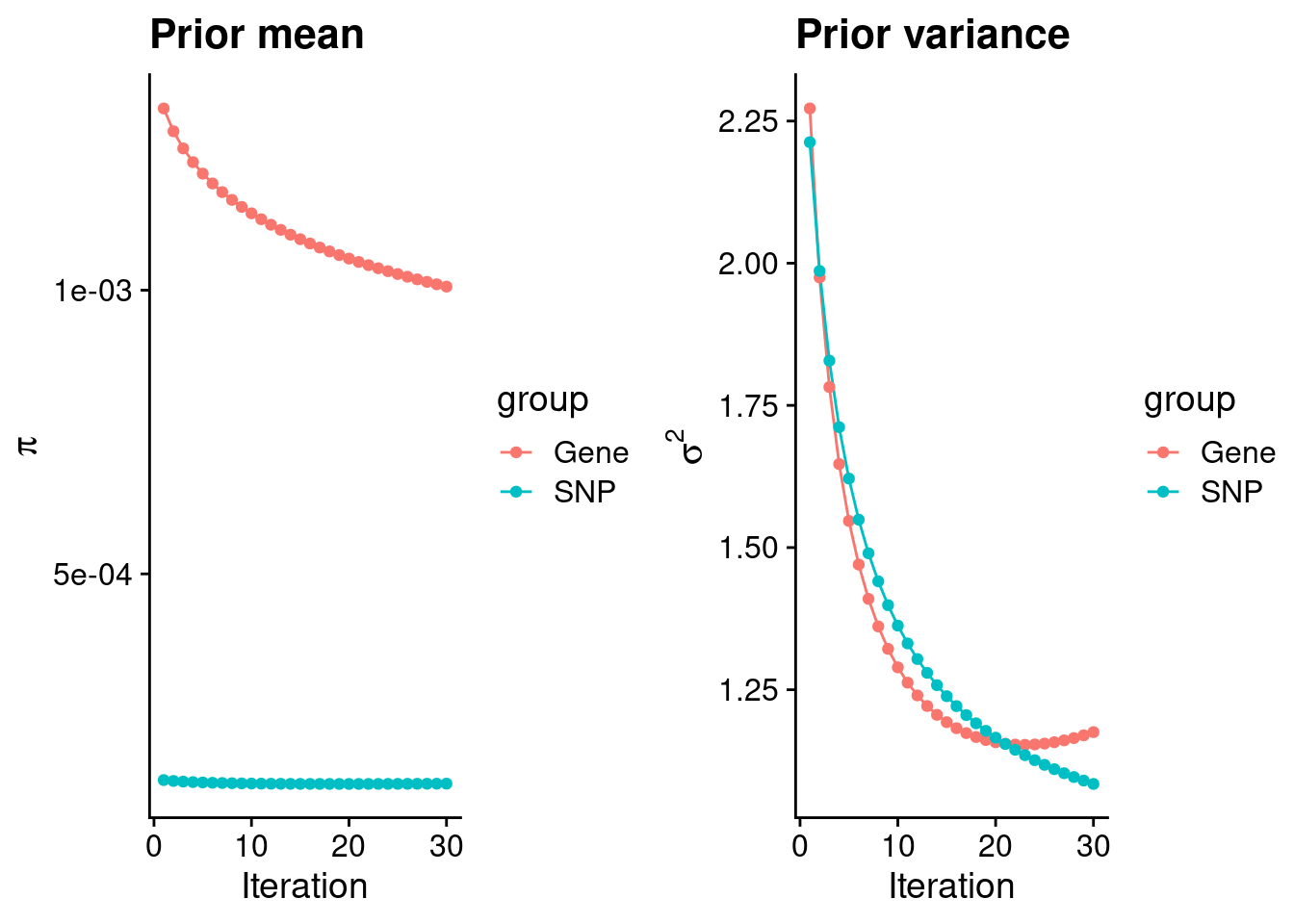

Version	Author	Date
dfd2b5f	wesleycrouse	2021-09-07

#estimated group prior
estimated_group_prior <- group_prior_rec[,ncol(group_prior_rec)]
names(estimated_group_prior) <- c("gene", "snp")
estimated_group_prior["snp"] <- estimated_group_prior["snp"]*thin #adjust parameter to account for thin argument
print(estimated_group_prior)

        gene          snp 
0.0010062774 0.0001304274

#estimated group prior variance
estimated_group_prior_var <- group_prior_var_rec[,ncol(group_prior_var_rec)]
names(estimated_group_prior_var) <- c("gene", "snp")
print(estimated_group_prior_var)

    gene      snp 
1.175389 1.084307

#report sample size
print(sample_size)

[1] 54498

#report group size
group_size <- c(nrow(ctwas_gene_res), n_snps)
print(group_size)

[1]   11095 8697330

#estimated group PVE
estimated_group_pve <- estimated_group_prior_var*estimated_group_prior*group_size/sample_size #check PVE calculation
names(estimated_group_pve) <- c("gene", "snp")
print(estimated_group_pve)

        gene          snp 
0.0002407942 0.0225697307

#compare sum(PIP*mu2/sample_size) with above PVE calculation
c(sum(ctwas_gene_res$PVE),sum(ctwas_snp_res$PVE))

[1] 0.004927462 0.466129415

Genes with highest PIPs

#distribution of PIPs
hist(ctwas_gene_res$susie_pip, xlim=c(0,1), main="Distribution of Gene PIPs")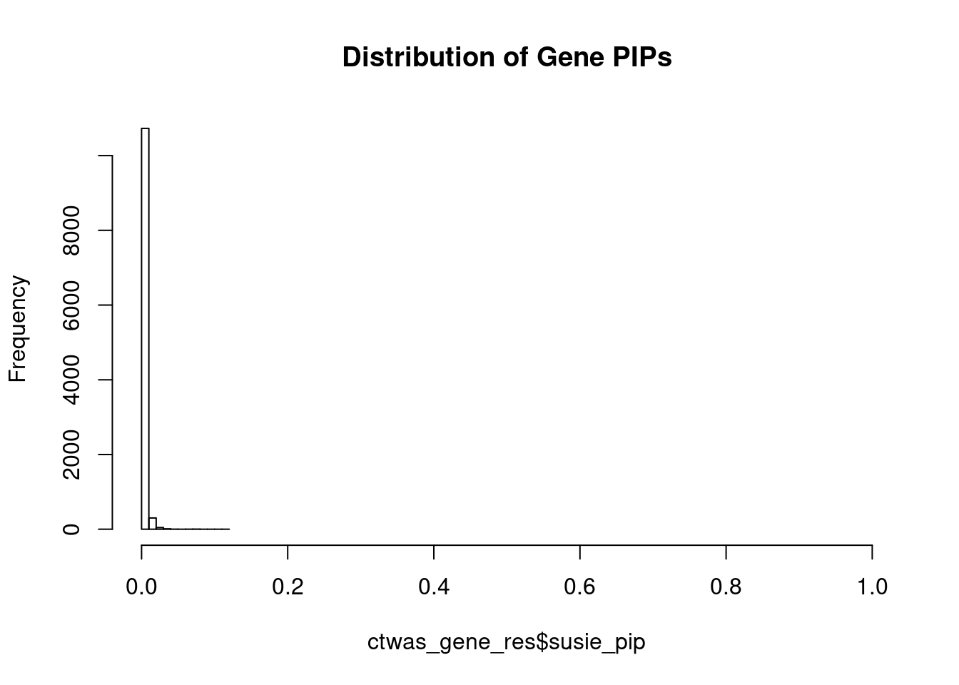

Version	Author	Date
dfd2b5f	wesleycrouse	2021-09-07

#genes with PIP>0.8 or 20 highest PIPs
head(ctwas_gene_res[order(-ctwas_gene_res$susie_pip),report_cols], max(sum(ctwas_gene_res$susie_pip>0.8), 20))

      genename region_tag susie_pip   mu2     PVE     z
4871      EPRS      1_112     0.119 22.34 4.9e-05  4.08
4142      GAMT       19_2     0.077 19.85 2.8e-05 -3.81
6002    GTF3C5       9_70     0.075 19.01 2.6e-05 -3.46
3122     AGMAT       1_11     0.074 19.48 2.7e-05 -3.57
4093    ATP1B2       17_7     0.069 20.83 2.6e-05 -4.72
2587     LIN7A      12_49     0.066 18.66 2.3e-05  3.42
4992     NUMA1      11_40     0.053 17.61 1.7e-05  3.42
82        GDE1      16_18     0.047 17.14 1.5e-05 -3.69
7164  SLC16A14      2_135     0.041 17.01 1.3e-05 -3.47
7143    TRIM17      1_116     0.039 15.68 1.1e-05 -3.23
6195     CCDC3      10_12     0.036 17.21 1.1e-05  3.20
4340    DNAJB1      19_12     0.036 15.32 1.0e-05 -3.11
5230     NUP58       13_6     0.034 15.36 9.7e-06 -3.00
1685     TCFL5      20_37     0.034 14.91 9.2e-06 -3.04
3979      VIL1      2_129     0.033 15.09 9.1e-06 -3.24
10836    HLA-C       6_26     0.033 25.29 1.5e-05 -4.99
4181  C6orf203       6_71     0.033 14.81 8.9e-06  3.09
2841    PDGFRB       5_88     0.032 14.55 8.4e-06  2.93
1424      MTAP       9_16     0.032 14.86 8.7e-06  2.95
11649   MIATNB       22_8     0.032 14.79 8.6e-06  2.93

Genes with largest effect sizes

#plot PIP vs effect size
plot(ctwas_gene_res$susie_pip, ctwas_gene_res$mu2, xlab="PIP", ylab="mu^2", main="Gene PIPs vs Effect Size")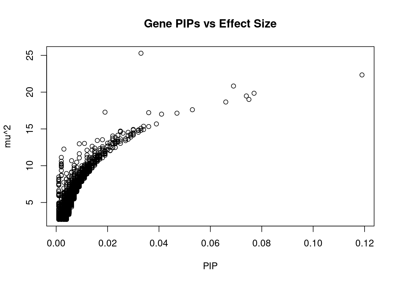

Version	Author	Date
dfd2b5f	wesleycrouse	2021-09-07

#genes with 20 largest effect sizes
head(ctwas_gene_res[order(-ctwas_gene_res$mu2),report_cols],20)

      genename region_tag susie_pip   mu2     PVE     z
10836    HLA-C       6_26     0.033 25.29 1.5e-05 -4.99
4871      EPRS      1_112     0.119 22.34 4.9e-05  4.08
4093    ATP1B2       17_7     0.069 20.83 2.6e-05 -4.72
4142      GAMT       19_2     0.077 19.85 2.8e-05 -3.81
3122     AGMAT       1_11     0.074 19.48 2.7e-05 -3.57
6002    GTF3C5       9_70     0.075 19.01 2.6e-05 -3.46
2587     LIN7A      12_49     0.066 18.66 2.3e-05  3.42
4992     NUMA1      11_40     0.053 17.61 1.7e-05  3.42
6527   ADAMTS3       4_52     0.019 17.28 6.0e-06 -3.25
6195     CCDC3      10_12     0.036 17.21 1.1e-05  3.20
82        GDE1      16_18     0.047 17.14 1.5e-05 -3.69
7164  SLC16A14      2_135     0.041 17.01 1.3e-05 -3.47
7143    TRIM17      1_116     0.039 15.68 1.1e-05 -3.23
5230     NUP58       13_6     0.034 15.36 9.7e-06 -3.00
4340    DNAJB1      19_12     0.036 15.32 1.0e-05 -3.11
3979      VIL1      2_129     0.033 15.09 9.1e-06 -3.24
7389    MAD2L1       4_78     0.030 14.93 8.1e-06  2.96
1685     TCFL5      20_37     0.034 14.91 9.2e-06 -3.04
1424      MTAP       9_16     0.032 14.86 8.7e-06  2.95
6970     PGAP3      17_23     0.030 14.85 8.2e-06 -3.42

Genes with highest PVE

#genes with 20 highest pve
head(ctwas_gene_res[order(-ctwas_gene_res$PVE),report_cols],20)

      genename region_tag susie_pip   mu2     PVE     z
4871      EPRS      1_112     0.119 22.34 4.9e-05  4.08
4142      GAMT       19_2     0.077 19.85 2.8e-05 -3.81
3122     AGMAT       1_11     0.074 19.48 2.7e-05 -3.57
6002    GTF3C5       9_70     0.075 19.01 2.6e-05 -3.46
4093    ATP1B2       17_7     0.069 20.83 2.6e-05 -4.72
2587     LIN7A      12_49     0.066 18.66 2.3e-05  3.42
4992     NUMA1      11_40     0.053 17.61 1.7e-05  3.42
10836    HLA-C       6_26     0.033 25.29 1.5e-05 -4.99
82        GDE1      16_18     0.047 17.14 1.5e-05 -3.69
7164  SLC16A14      2_135     0.041 17.01 1.3e-05 -3.47
7143    TRIM17      1_116     0.039 15.68 1.1e-05 -3.23
6195     CCDC3      10_12     0.036 17.21 1.1e-05  3.20
4340    DNAJB1      19_12     0.036 15.32 1.0e-05 -3.11
5230     NUP58       13_6     0.034 15.36 9.7e-06 -3.00
1685     TCFL5      20_37     0.034 14.91 9.2e-06 -3.04
3979      VIL1      2_129     0.033 15.09 9.1e-06 -3.24
4181  C6orf203       6_71     0.033 14.81 8.9e-06  3.09
1424      MTAP       9_16     0.032 14.86 8.7e-06  2.95
11649   MIATNB       22_8     0.032 14.79 8.6e-06  2.93
2841    PDGFRB       5_88     0.032 14.55 8.4e-06  2.93

Genes with largest z scores

#genes with 20 largest z scores
head(ctwas_gene_res[order(-abs(ctwas_gene_res$z)),report_cols],20)

       genename region_tag susie_pip   mu2     PVE     z
10836     HLA-C       6_26     0.033 25.29 1.5e-05 -4.99
4093     ATP1B2       17_7     0.069 20.83 2.6e-05 -4.72
4871       EPRS      1_112     0.119 22.34 4.9e-05  4.08
7001     ALOX15       17_4     0.024 14.14 6.1e-06  4.00
5423      ARRB2       17_4     0.022 13.75 5.6e-06 -3.96
4142       GAMT       19_2     0.077 19.85 2.8e-05 -3.81
11526   TNFSF12       17_7     0.012 11.46 2.6e-06  3.75
82         GDE1      16_18     0.047 17.14 1.5e-05 -3.69
3122      AGMAT       1_11     0.074 19.48 2.7e-05 -3.57
7164   SLC16A14      2_135     0.041 17.01 1.3e-05 -3.47
6002     GTF3C5       9_70     0.075 19.01 2.6e-05 -3.46
4992      NUMA1      11_40     0.053 17.61 1.7e-05  3.42
2587      LIN7A      12_49     0.066 18.66 2.3e-05  3.42
6970      PGAP3      17_23     0.030 14.85 8.2e-06 -3.42
5463      MIEN1      17_23     0.028 14.54 7.6e-06  3.38
6527    ADAMTS3       4_52     0.019 17.28 6.0e-06 -3.25
3979       VIL1      2_129     0.033 15.09 9.1e-06 -3.24
7143     TRIM17      1_116     0.039 15.68 1.1e-05 -3.23
11997 LINC01963      2_127     0.030 14.47 7.8e-06 -3.21
4269   ATP6V1E1       22_2     0.020 13.06 4.9e-06 -3.21

Comparing z scores and PIPs

#set nominal signifiance threshold for z scores
alpha <- 0.05

#bonferroni adjusted threshold for z scores
sig_thresh <- qnorm(1-(alpha/nrow(ctwas_gene_res)/2), lower=T)

#Q-Q plot for z scores
obs_z <- ctwas_gene_res$z[order(ctwas_gene_res$z)]
exp_z <- qnorm((1:nrow(ctwas_gene_res))/nrow(ctwas_gene_res))

plot(exp_z, obs_z, xlab="Expected z", ylab="Observed z", main="Gene z score Q-Q plot")
abline(a=0,b=1)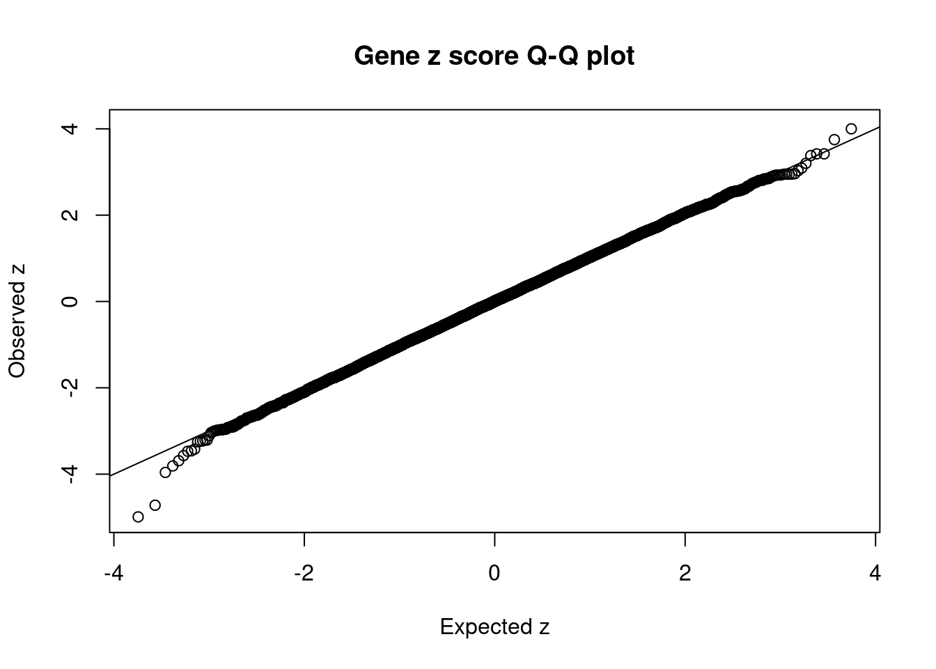

Version	Author	Date
dfd2b5f	wesleycrouse	2021-09-07

#plot z score vs PIP
plot(abs(ctwas_gene_res$z), ctwas_gene_res$susie_pip, xlab="abs(z)", ylab="PIP")
abline(v=sig_thresh, col="red", lty=2)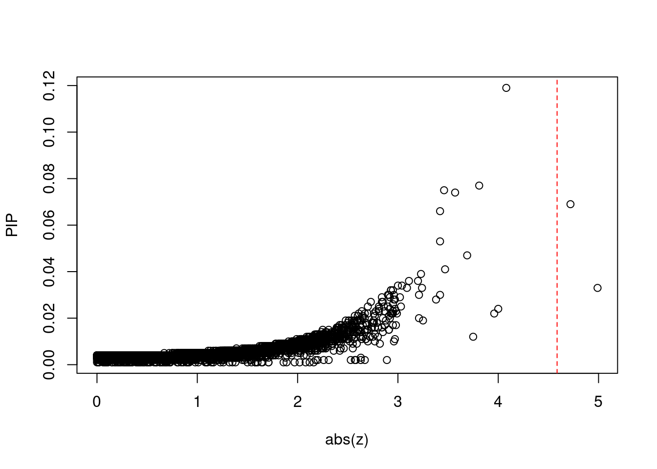

Version	Author	Date
dfd2b5f	wesleycrouse	2021-09-07

#proportion of significant z scores
mean(abs(ctwas_gene_res$z) > sig_thresh)

[1] 0.0001802614

#genes with most significant z scores
head(ctwas_gene_res[order(-abs(ctwas_gene_res$z)),report_cols],20)

       genename region_tag susie_pip   mu2     PVE     z
10836     HLA-C       6_26     0.033 25.29 1.5e-05 -4.99
4093     ATP1B2       17_7     0.069 20.83 2.6e-05 -4.72
4871       EPRS      1_112     0.119 22.34 4.9e-05  4.08
7001     ALOX15       17_4     0.024 14.14 6.1e-06  4.00
5423      ARRB2       17_4     0.022 13.75 5.6e-06 -3.96
4142       GAMT       19_2     0.077 19.85 2.8e-05 -3.81
11526   TNFSF12       17_7     0.012 11.46 2.6e-06  3.75
82         GDE1      16_18     0.047 17.14 1.5e-05 -3.69
3122      AGMAT       1_11     0.074 19.48 2.7e-05 -3.57
7164   SLC16A14      2_135     0.041 17.01 1.3e-05 -3.47
6002     GTF3C5       9_70     0.075 19.01 2.6e-05 -3.46
4992      NUMA1      11_40     0.053 17.61 1.7e-05  3.42
2587      LIN7A      12_49     0.066 18.66 2.3e-05  3.42
6970      PGAP3      17_23     0.030 14.85 8.2e-06 -3.42
5463      MIEN1      17_23     0.028 14.54 7.6e-06  3.38
6527    ADAMTS3       4_52     0.019 17.28 6.0e-06 -3.25
3979       VIL1      2_129     0.033 15.09 9.1e-06 -3.24
7143     TRIM17      1_116     0.039 15.68 1.1e-05 -3.23
11997 LINC01963      2_127     0.030 14.47 7.8e-06 -3.21
4269   ATP6V1E1       22_2     0.020 13.06 4.9e-06 -3.21

Locus plots for genes and SNPs

ctwas_gene_res_sortz <- ctwas_gene_res[order(-abs(ctwas_gene_res$z)),]

n_plots <- 5
for (region_tag_plot in head(unique(ctwas_gene_res_sortz$region_tag), n_plots)){
  ctwas_res_region <-  ctwas_res[ctwas_res$region_tag==region_tag_plot,]
  start <- min(ctwas_res_region$pos)
  end <- max(ctwas_res_region$pos)
  
  ctwas_res_region <- ctwas_res_region[order(ctwas_res_region$pos),]
  ctwas_res_region_gene <- ctwas_res_region[ctwas_res_region$type=="gene",]
  ctwas_res_region_snp <- ctwas_res_region[ctwas_res_region$type=="SNP",]
  
  #region name
  print(paste0("Region: ", region_tag_plot))
  
  #table of genes in region
  print(ctwas_res_region_gene[,report_cols])
  
  par(mfrow=c(4,1))
  
  #gene z scores
  plot(ctwas_res_region_gene$pos, abs(ctwas_res_region_gene$z), xlab="Position", ylab="abs(gene_z)", xlim=c(start,end),
   ylim=c(0,max(sig_thresh, abs(ctwas_res_region_gene$z))),
   main=paste0("Region: ", region_tag_plot))
  abline(h=sig_thresh,col="red",lty=2)
  
  #significance threshold for SNPs
  alpha_snp <- 5*10^(-8)
  sig_thresh_snp <- qnorm(1-alpha_snp/2, lower=T)
  
  #snp z scores
  plot(ctwas_res_region_snp$pos, abs(ctwas_res_region_snp$z), xlab="Position", ylab="abs(snp_z)",xlim=c(start,end),
   ylim=c(0,max(sig_thresh_snp, max(abs(ctwas_res_region_snp$z)))))
  abline(h=sig_thresh_snp,col="purple",lty=2)
  
  #gene pips
  plot(ctwas_res_region_gene$pos, ctwas_res_region_gene$susie_pip, xlab="Position", ylab="Gene PIP", xlim=c(start,end), ylim=c(0,1))
  abline(h=0.8,col="blue",lty=2)
  
  #snp pips
  plot(ctwas_res_region_snp$pos, ctwas_res_region_snp$susie_pip, xlab="Position", ylab="SNP PIP", xlim=c(start,end), ylim=c(0,1))
  abline(h=0.8,col="blue",lty=2)
}

[1] "Region: 6_26"
               genename region_tag susie_pip   mu2     PVE     z
10855             HLA-G       6_26     0.001  3.19 3.3e-08  0.80
12599             HCP5B       6_26     0.002 10.60 4.3e-07 -2.67
10968             HLA-A       6_26     0.001  4.80 6.7e-08  1.35
10853              HCG9       6_26     0.001  4.91 7.0e-08  1.38
10851           PPP1R11       6_26     0.001  3.32 3.5e-08  0.81
661               ZNRD1       6_26     0.001  2.72 2.6e-08  0.15
10850             RNF39       6_26     0.001  3.69 4.2e-08 -0.86
10848            TRIM10       6_26     0.002 10.19 3.8e-07  2.58
10847            TRIM15       6_26     0.001  2.74 2.6e-08 -0.15
11418            TRIM26       6_26     0.001  3.54 3.9e-08 -0.89
10845            TRIM39       6_26     0.001  6.05 1.1e-07  1.71
11563             RPP21       6_26     0.001  3.40 3.7e-08 -0.68
10844             HLA-E       6_26     0.001  3.96 4.7e-08 -1.10
10841           MRPS18B       6_26     0.001  3.66 4.1e-08  0.90
10840          C6orf136       6_26     0.002 10.02 3.7e-07  2.53
10839             DHX16       6_26     0.001  3.95 4.7e-08 -0.91
5868            PPP1R18       6_26     0.001  3.04 3.1e-08 -0.63
4976                NRM       6_26     0.001  2.85 2.8e-08 -0.28
4970              FLOT1       6_26     0.001  6.46 1.2e-07 -1.65
10230              TUBB       6_26     0.001  2.86 2.8e-08  0.32
4971               IER3       6_26     0.001  3.19 3.3e-08 -0.59
11120         LINC00243       6_26     0.001  4.69 6.4e-08 -1.32
10843              DDR1       6_26     0.001  3.26 3.4e-08  0.59
11052            GTF2H4       6_26     0.001  3.20 3.3e-08  0.73
4978              VARS2       6_26     0.001  4.94 7.1e-08  1.58
10838            CCHCR1       6_26     0.002  9.83 3.5e-07 -2.63
4969              TCF19       6_26     0.001  2.70 2.6e-08 -0.08
10966             HCG27       6_26     0.002 10.27 3.9e-07  2.89
10837            POU5F1       6_26     0.001  3.00 3.0e-08 -0.47
10836             HLA-C       6_26     0.033 25.29 1.5e-05 -4.99
10788            NOTCH4       6_26     0.001  2.79 2.7e-08  0.21
11439             HLA-B       6_26     0.001  2.81 2.7e-08 -0.42
12270 XXbac-BPG181B23.7       6_26     0.001  2.90 2.8e-08 -0.47
10834              MICA       6_26     0.001  3.17 3.3e-08 -0.63
10833              MICB       6_26     0.001  3.25 3.4e-08 -0.43
10830              LST1       6_26     0.001  2.70 2.6e-08  0.00
10619            DDX39B       6_26     0.001  3.15 3.2e-08  0.63
11050          ATP6V1G2       6_26     0.001  4.49 5.9e-08  1.50
10831           NFKBIL1       6_26     0.001  2.72 2.6e-08  0.11
11282               LTA       6_26     0.001  2.98 3.0e-08  0.52
11296               LTB       6_26     0.001  2.99 3.0e-08  0.53
11395               TNF       6_26     0.001  4.43 5.8e-08 -1.09
10829              NCR3       6_26     0.001  4.15 5.1e-08 -1.14
10828              AIF1       6_26     0.001  4.73 6.5e-08  1.16
10827            PRRC2A       6_26     0.001  5.94 1.0e-07  1.60
10826              BAG6       6_26     0.001  2.87 2.8e-08 -0.35
10825              APOM       6_26     0.002 11.13 5.0e-07  2.57
10824           C6orf47       6_26     0.001  4.49 5.9e-08  1.16
10822            CSNK2B       6_26     0.001  6.65 1.3e-07 -1.71
10823            GPANK1       6_26     0.001  5.92 1.0e-07  1.58
11539            LY6G5B       6_26     0.001  2.76 2.6e-08 -0.27
10821            LY6G5C       6_26     0.001  2.72 2.6e-08  0.07
11639            LY6G6D       6_26     0.001  2.91 2.9e-08 -0.44
10818            MPIG6B       6_26     0.001  2.82 2.7e-08  0.30
10819            LY6G6C       6_26     0.001  4.81 6.7e-08 -1.26
11048             DDAH2       6_26     0.001  4.58 6.1e-08 -1.23
10817              MSH5       6_26     0.001  4.03 4.9e-08 -0.98
11047             CLIC1       6_26     0.002  9.36 3.0e-07  2.31
11327            SAPCD1       6_26     0.003 12.26 6.8e-07 -2.63
10814              VWA7       6_26     0.001  3.46 3.8e-08 -0.73
10809           C6orf48       6_26     0.001  4.11 5.0e-08 -1.01
10813              VARS       6_26     0.001  2.79 2.7e-08 -0.24
10812              LSM2       6_26     0.001  2.84 2.8e-08 -0.32
10811            HSPA1L       6_26     0.001  2.71 2.6e-08 -0.06
10808              NEU1       6_26     0.002  8.70 2.5e-07  2.20
10807           SLC44A4       6_26     0.002  8.65 2.5e-07 -2.18
7712                 C2       6_26     0.001  8.47 2.3e-07 -2.16
10805             EHMT2       6_26     0.001  7.35 1.6e-07 -1.89
10802             NELFE       6_26     0.001  5.98 1.0e-07 -1.54
10801            SKIV2L       6_26     0.001  6.19 1.1e-07  1.64
10797             STK19       6_26     0.002  9.99 3.6e-07  2.26
10800               DXO       6_26     0.001  3.74 4.3e-08  0.84
11652               C4A       6_26     0.001  8.17 2.1e-07  2.12
11218               C4B       6_26     0.001  7.42 1.7e-07 -1.97
11374           CYP21A2       6_26     0.001  2.78 2.7e-08  0.15
11193              PPT2       6_26     0.001  4.11 5.0e-08 -1.08
11043             ATF6B       6_26     0.001  7.54 1.7e-07  1.86
10795             FKBPL       6_26     0.001  2.99 3.0e-08 -0.41
10794             PRRT1       6_26     0.001  3.03 3.0e-08  0.46
10791              RNF5       6_26     0.001  2.89 2.8e-08  0.32
11565             EGFL8       6_26     0.001  6.09 1.1e-07 -1.58
10792            AGPAT1       6_26     0.001  3.44 3.7e-08 -0.70
10790              AGER       6_26     0.001  8.09 2.1e-07 -2.08
10789              PBX2       6_26     0.001  2.78 2.7e-08  0.32
10608          HLA-DRB5       6_26     0.001  7.87 1.9e-07 -2.02
10325          HLA-DQA1       6_26     0.001  3.81 4.4e-08 -0.92
11490          HLA-DQA2       6_26     0.001  3.25 3.4e-08  0.72
11389          HLA-DQB2       6_26     0.001  2.86 2.8e-08 -0.33
9260           HLA-DQB1       6_26     0.001  2.77 2.7e-08  0.22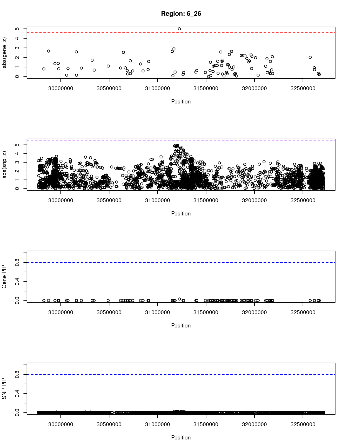

Version	Author	Date
dfd2b5f	wesleycrouse	2021-09-07

[1] "Region: 17_7"
        genename region_tag susie_pip   mu2     PVE     z
7010       FGF11       17_7     0.014 12.14 3.1e-06 -2.59
8293      CHRNB1       17_7     0.002  2.75 1.3e-07 -0.39
9403      POLR2A       17_7     0.003  3.94 2.2e-07  1.40
11526    TNFSF12       17_7     0.012 11.46 2.6e-06  3.75
7008     TNFSF13       17_7     0.003  3.75 2.1e-07 -0.81
7009       SENP3       17_7     0.003  3.69 2.0e-07 -0.61
4096       MPDU1       17_7     0.003  4.18 2.5e-07  0.75
5427        SAT2       17_7     0.003  2.89 1.4e-07  0.35
4093      ATP1B2       17_7     0.069 20.83 2.6e-05 -4.72
5425      WRAP53       17_7     0.006  7.21 7.5e-07 -2.14
5430        TP53       17_7     0.003  3.43 1.8e-07 -0.53
4402       KDM6B       17_7     0.002  2.72 1.2e-07 -0.31
7989      TMEM88       17_7     0.003  4.11 2.4e-07  1.09
9555       NAA38       17_7     0.005  5.97 5.0e-07  1.57
8272        CHD3       17_7     0.003  2.89 1.4e-07 -0.39
9286  AC025335.1       17_7     0.003  3.59 1.9e-07  0.90
8279      KCNAB3       17_7     0.002  2.70 1.2e-07 -0.07
8277      CNTROB       17_7     0.003  2.93 1.4e-07 -0.44
8278     TRAPPC1       17_7     0.003  2.91 1.4e-07 -0.34
11172      VAMP2       17_7     0.002  2.71 1.2e-07  0.05
9234     TMEM107       17_7     0.003  4.22 2.5e-07  1.01
10292     BORCS6       17_7     0.002  2.75 1.3e-07  0.17
9228   LINC00324       17_7     0.002  2.70 1.2e-07  0.04
9218        PFAS       17_7     0.015 12.39 3.4e-06  2.60
9226        CTC1       17_7     0.002  2.74 1.3e-07  0.19
3790    SLC25A35       17_7     0.003  2.78 1.3e-07  0.24
9716       KRBA2       17_7     0.003  2.83 1.3e-07 -0.33
7011       RPL26       17_7     0.003  4.27 2.6e-07  1.07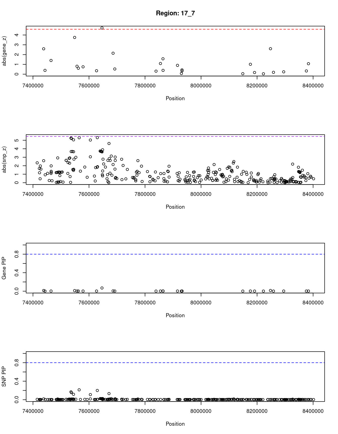

Version	Author	Date
dfd2b5f	wesleycrouse	2021-09-07

[1] "Region: 1_112"
           genename region_tag susie_pip   mu2     PVE     z
4871           EPRS      1_112     0.119 22.34 4.9e-05  4.08
7125          BPNT1      1_112     0.003  2.78 1.7e-07  0.25
691           IARS2      1_112     0.003  2.93 1.9e-07  0.36
3289       RAB3GAP2      1_112     0.003  2.96 1.9e-07  0.50
7126       C1orf115      1_112     0.007  6.45 7.8e-07  1.66
3225          MARC2      1_112     0.004  3.47 2.4e-07 -0.69
9905          MARC1      1_112     0.003  2.99 1.9e-07 -0.44
11173   RNU6ATAC35P      1_112     0.004  3.80 2.8e-07  0.93
11507     LINC01352      1_112     0.005  4.77 4.3e-07  1.24
12333 RP11-295M18.6      1_112     0.004  3.71 2.7e-07  0.87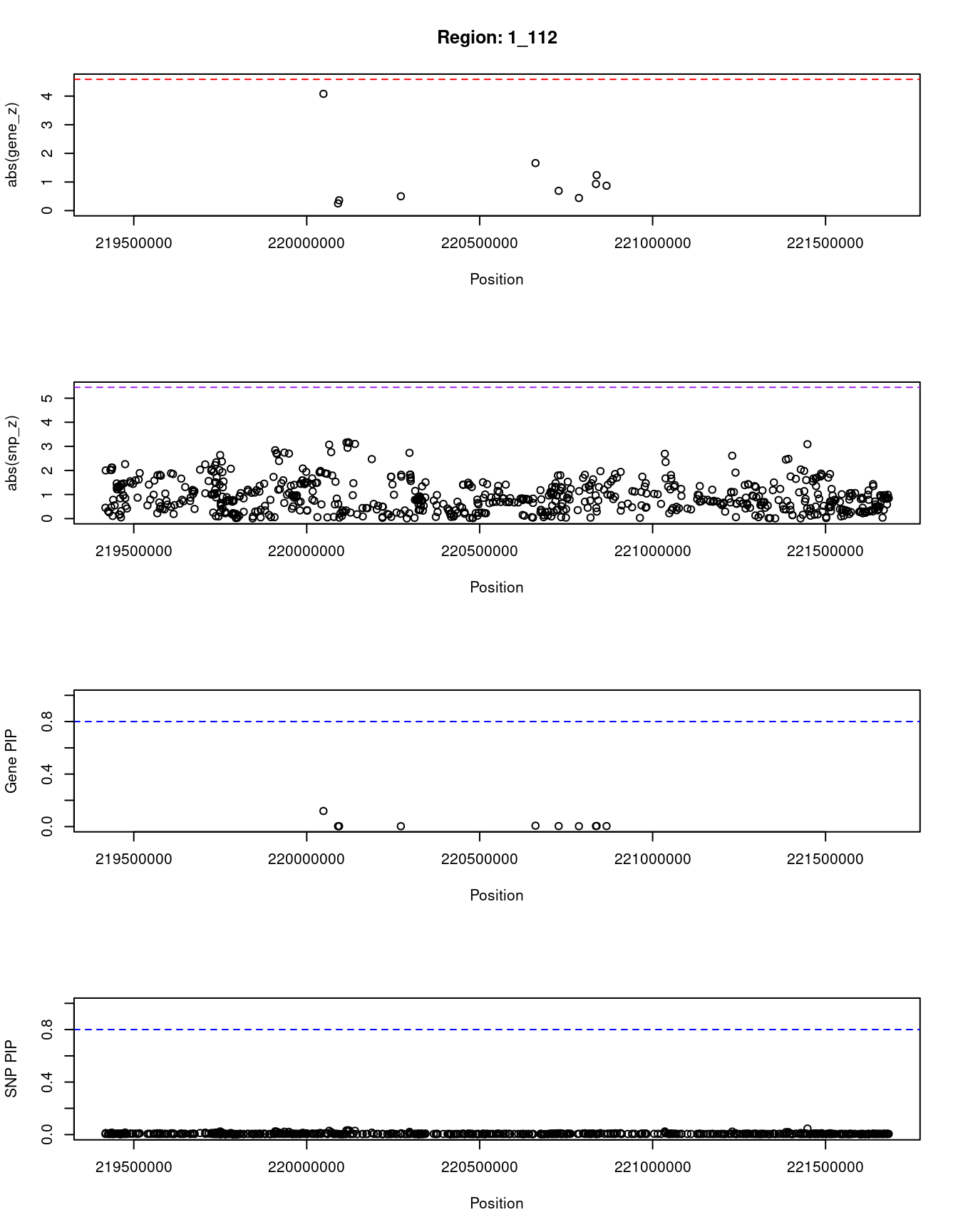

Version	Author	Date
dfd2b5f	wesleycrouse	2021-09-07

[1] "Region: 17_4"
     genename region_tag susie_pip   mu2     PVE     z
1058    ITGAE       17_4     0.005  5.68 5.2e-07  1.42
850     NCBP3       17_4     0.003  3.44 2.1e-07  0.72
39     CAMKK1       17_4     0.007  7.78 1.0e-06 -1.87
2367    P2RX1       17_4     0.003  2.95 1.6e-07  0.42
851    ATP2A3       17_4     0.003  3.15 1.8e-07  0.59
861     ZZEF1       17_4     0.003  2.81 1.5e-07 -0.33
7964   CYB5D2       17_4     0.003  3.76 2.4e-07 -0.96
4383   UBE2G1       17_4     0.005  5.35 4.6e-07  1.49
9512    SPNS3       17_4     0.005  5.32 4.6e-07 -1.32
9556    SPNS2       17_4     0.005  5.61 5.1e-07  1.47
4380  MYBBP1A       17_4     0.003  3.49 2.1e-07  0.69
7001   ALOX15       17_4     0.024 14.14 6.1e-06  4.00
5423    ARRB2       17_4     0.022 13.75 5.6e-06 -3.96
5424  ZMYND15       17_4     0.004  5.10 4.2e-07 -1.78
7004   CXCL16       17_4     0.003  3.65 2.3e-07 -1.13
7003    MED11       17_4     0.003  3.35 2.0e-07 -0.96
9494   GLTPD2       17_4     0.013 10.89 2.6e-06  2.46
9538     VMO1       17_4     0.006  6.37 6.6e-07 -1.71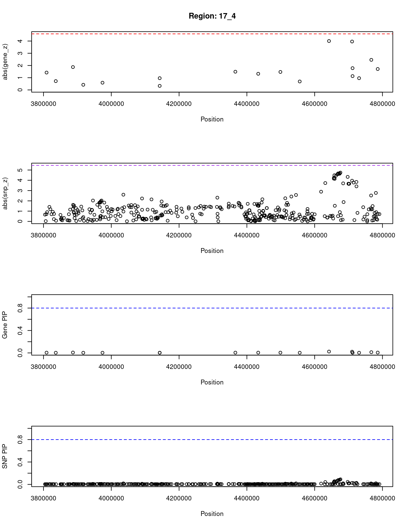

Version	Author	Date
dfd2b5f	wesleycrouse	2021-09-07

[1] "Region: 19_2"
         genename region_tag susie_pip   mu2     PVE     z
1427       POLRMT       19_2     0.004  3.78 2.8e-07  0.88
12142  AC004156.3       19_2     0.004  3.18 2.1e-07 -0.58
750         FSTL3       19_2     0.004  4.15 3.3e-07 -1.00
9774       PRSS57       19_2     0.004  3.18 2.1e-07  0.58
1433         PALM       19_2     0.004  4.29 3.5e-07  1.06
201         PTBP1       19_2     0.013 10.26 2.5e-06 -2.34
10454       ELANE       19_2     0.005  4.49 3.8e-07 -1.13
10484         CFD       19_2     0.005  4.67 4.1e-07 -1.22
8877        MED16       19_2     0.004  3.75 2.8e-07 -0.91
3051       KISS1R       19_2     0.006  5.62 5.9e-07 -1.48
3053       ARID3A       19_2     0.014 10.36 2.6e-06 -2.36
9465      TMEM259       19_2     0.006  5.79 6.3e-07  1.52
602          CNN2       19_2     0.007  6.75 8.7e-07  1.73
603         ABCA7       19_2     0.005  4.36 3.6e-07  1.15
3055       GRIN3B       19_2     0.004  3.30 2.3e-07  0.70
9341     ARHGAP45       19_2     0.003  2.70 1.7e-07  0.03
1426       POLR2E       19_2     0.004  3.22 2.2e-07  0.65
7901         GPX4       19_2     0.003  2.71 1.7e-07 -0.08
609         SBNO2       19_2     0.008  7.10 9.8e-07  1.76
1417        ATP5D       19_2     0.003  2.87 1.8e-07  0.33
11311    C19orf24       19_2     0.003  2.78 1.7e-07 -0.24
6939         MUM1       19_2     0.003  2.87 1.8e-07 -0.32
4142         GAMT       19_2     0.077 19.85 2.8e-05 -3.81
3336     C19orf25       19_2     0.003  2.75 1.7e-07 -0.19
2960        PCSK4       19_2     0.003  2.72 1.7e-07  0.13
2959        REEP6       19_2     0.003  2.70 1.7e-07 -0.01
783          MBD3       19_2     0.004  3.52 2.5e-07  0.76
3964       UQCR11       19_2     0.003  2.79 1.7e-07 -0.26
781          TCF3       19_2     0.006  5.47 5.6e-07 -1.40
4168       ATP8B3       19_2     0.004  3.02 2.0e-07 -0.48
980         REXO1       19_2     0.003  2.88 1.8e-07  0.37
12032 CTB-31O20.2       19_2     0.003  2.91 1.9e-07  0.37
11294      SCAMP4       19_2     0.004  3.41 2.4e-07 -0.70
4484      CSNK1G2       19_2     0.007  6.81 8.9e-07 -1.70
4479        BTBD2       19_2     0.004  3.70 2.7e-07  0.85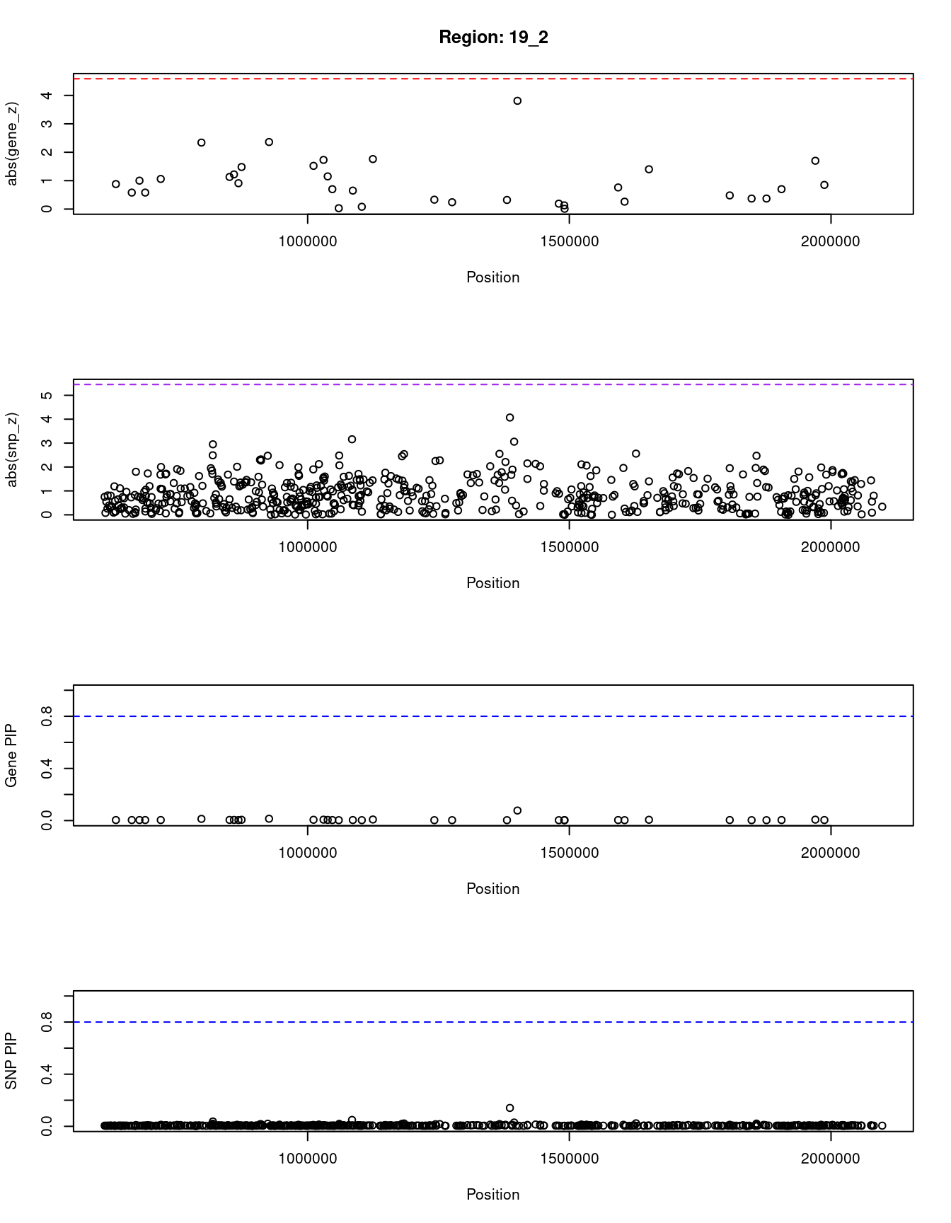

Version	Author	Date
dfd2b5f	wesleycrouse	2021-09-07

SNPs with highest PIPs

#snps with PIP>0.8 or 20 highest PIPs
head(ctwas_snp_res[order(-ctwas_snp_res$susie_pip),report_cols_snps],
max(sum(ctwas_snp_res$susie_pip>0.8), 20))

                id region_tag susie_pip   mu2     PVE     z
396298  rs62444120       7_28     0.231 23.37 9.9e-05 -4.35
140037  rs75620930        3_1     0.230 23.43 9.9e-05  4.34
761470   rs4968212       17_7     0.213 24.80 9.7e-05 -5.30
476904 rs112371525       8_89     0.208 22.82 8.7e-05  4.23
761480  rs62059839       17_7     0.199 24.43 8.9e-05  5.31
679108   rs1959607       14_1     0.192 22.43 7.9e-05  4.21
526099 rs551737161      10_16     0.176 23.42 7.6e-05  3.60
813811  rs73000658      19_16     0.174 21.69 6.9e-05 -4.06
761458   rs9892862       17_7     0.169 23.48 7.3e-05  5.26
319306  rs13160700      5_104     0.166 21.87 6.7e-05 -4.06
165332   rs9813399       3_53     0.165 21.26 6.4e-05  4.14
70306   rs13429539        2_7     0.162 22.24 6.6e-05 -4.12
513886  rs10760461       9_65     0.158 21.52 6.2e-05  4.10
417774    rs876169       7_68     0.156 21.39 6.1e-05  4.31
761460   rs8073177       17_7     0.153 22.95 6.4e-05  5.21
272419 rs112157462       5_14     0.151 20.93 5.8e-05  3.98
459963 rs553564201       8_57     0.150 21.44 5.9e-05  3.99
154020  rs76750610       3_28     0.146 20.73 5.5e-05 -3.93
381048 rs113784847        7_3     0.143 21.31 5.6e-05 -4.04
2845     rs2274332        1_6     0.141 20.57 5.3e-05 -3.89

SNPs with largest effect sizes

#plot PIP vs effect size
plot(ctwas_snp_res$susie_pip, ctwas_snp_res$mu2, xlab="PIP", ylab="mu^2", main="SNP PIPs vs Effect Size")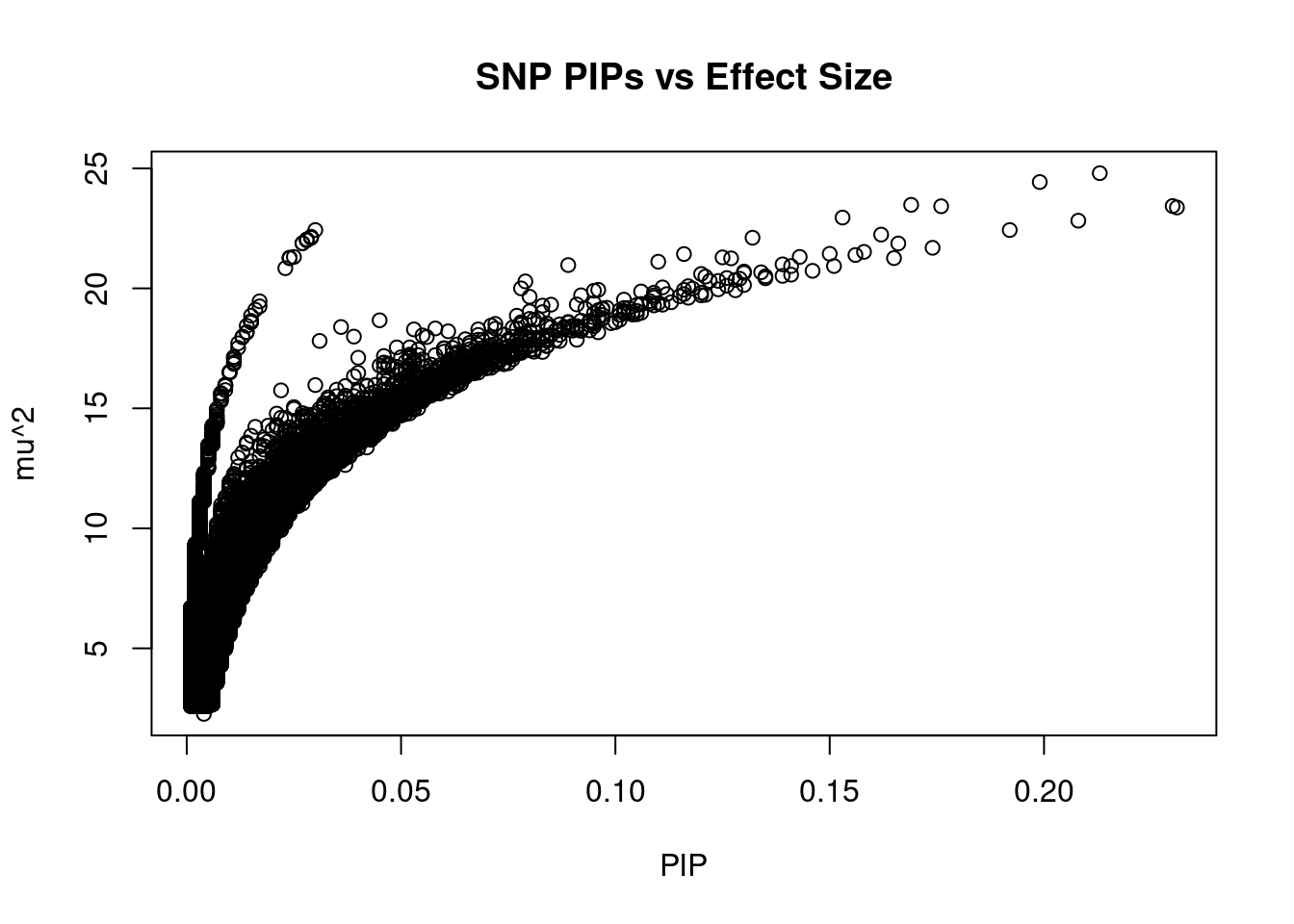

Version	Author	Date
dfd2b5f	wesleycrouse	2021-09-07

#SNPs with 50 largest effect sizes
head(ctwas_snp_res[order(-ctwas_snp_res$mu2),report_cols_snps],50)

                id region_tag susie_pip   mu2     PVE     z
761470   rs4968212       17_7     0.213 24.80 9.7e-05 -5.30
761480  rs62059839       17_7     0.199 24.43 8.9e-05  5.31
761458   rs9892862       17_7     0.169 23.48 7.3e-05  5.26
140037  rs75620930        3_1     0.230 23.43 9.9e-05  4.34
526099 rs551737161      10_16     0.176 23.42 7.6e-05  3.60
396298  rs62444120       7_28     0.231 23.37 9.9e-05 -4.35
761460   rs8073177       17_7     0.153 22.95 6.4e-05  5.21
476904 rs112371525       8_89     0.208 22.82 8.7e-05  4.23
333973   rs6913470       6_26     0.030 22.43 1.3e-05  4.92
679108   rs1959607       14_1     0.192 22.43 7.9e-05  4.21
70306   rs13429539        2_7     0.162 22.24 6.6e-05 -4.12
333928    rs915660       6_26     0.029 22.15 1.2e-05  4.89
333930   rs9357109       6_26     0.029 22.12 1.2e-05  4.88
761500   rs1641549       17_7     0.132 22.11 5.3e-05 -4.62
333967   rs7453202       6_26     0.029 22.10 1.2e-05  4.89
333971   rs6907451       6_26     0.028 22.04 1.1e-05  4.89
333957  rs28360066       6_26     0.028 22.02 1.1e-05  4.88
333964   rs9380223       6_26     0.028 22.00 1.1e-05  4.88
333953   rs9391819       6_26     0.027 21.88 1.1e-05  4.86
333960   rs9404983       6_26     0.027 21.88 1.1e-05  4.86
319306  rs13160700      5_104     0.166 21.87 6.7e-05 -4.06
813811  rs73000658      19_16     0.174 21.69 6.9e-05 -4.06
513886  rs10760461       9_65     0.158 21.52 6.2e-05  4.10
459963 rs553564201       8_57     0.150 21.44 5.9e-05  3.99
761464  rs11078694       17_7     0.116 21.43 4.6e-05 -5.05
417774    rs876169       7_68     0.156 21.39 6.1e-05  4.31
333947  rs28360062       6_26     0.025 21.31 9.6e-06  4.82
381048 rs113784847        7_3     0.143 21.31 5.6e-05 -4.04
39473  rs192164271       1_80     0.125 21.29 4.9e-05  3.94
333942   rs9378115       6_26     0.024 21.28 9.6e-06  4.81
165332   rs9813399       3_53     0.165 21.26 6.4e-05  4.14
333938   rs6899875       6_26     0.024 21.26 9.5e-06  4.81
333940   rs9357115       6_26     0.024 21.26 9.5e-06  4.81
138489   rs3791461      2_143     0.127 21.25 5.0e-05 -3.97
761474 rs149932962       17_7     0.110 21.11 4.3e-05  5.03
327669 rs192338591       6_13     0.139 21.00 5.4e-05  3.94
758122  rs11076740      16_54     0.089 20.97 3.4e-05 -3.98
272419 rs112157462       5_14     0.151 20.93 5.8e-05  3.98
806869 rs117700303       19_2     0.141 20.93 5.4e-05 -4.07
333976  rs17191237       6_26     0.023 20.84 8.6e-06  4.78
154020  rs76750610       3_28     0.146 20.73 5.5e-05 -3.93
742136 rs143894776      16_23     0.130 20.70 4.9e-05 -3.90
423042   rs9640863       7_80     0.134 20.67 5.1e-05 -3.96
96986  rs187600283       2_58     0.130 20.64 4.9e-05  3.88
642695 rs146568110      12_75     0.120 20.60 4.5e-05  3.84
2845     rs2274332        1_6     0.141 20.57 5.3e-05 -3.89
598854  rs73008432      11_70     0.139 20.52 5.2e-05  4.04
106803  rs62162215       2_78     0.135 20.50 5.1e-05 -3.94
182446   rs9823043       3_85     0.121 20.49 4.5e-05 -4.05
710597  rs76553406       15_9     0.126 20.43 4.7e-05  3.91

SNPs with highest PVE

#SNPs with 50 highest pve
head(ctwas_snp_res[order(-ctwas_snp_res$PVE),report_cols_snps],50)

                id region_tag susie_pip   mu2     PVE     z
140037  rs75620930        3_1     0.230 23.43 9.9e-05  4.34
396298  rs62444120       7_28     0.231 23.37 9.9e-05 -4.35
761470   rs4968212       17_7     0.213 24.80 9.7e-05 -5.30
761480  rs62059839       17_7     0.199 24.43 8.9e-05  5.31
476904 rs112371525       8_89     0.208 22.82 8.7e-05  4.23
679108   rs1959607       14_1     0.192 22.43 7.9e-05  4.21
526099 rs551737161      10_16     0.176 23.42 7.6e-05  3.60
761458   rs9892862       17_7     0.169 23.48 7.3e-05  5.26
813811  rs73000658      19_16     0.174 21.69 6.9e-05 -4.06
319306  rs13160700      5_104     0.166 21.87 6.7e-05 -4.06
70306   rs13429539        2_7     0.162 22.24 6.6e-05 -4.12
165332   rs9813399       3_53     0.165 21.26 6.4e-05  4.14
761460   rs8073177       17_7     0.153 22.95 6.4e-05  5.21
513886  rs10760461       9_65     0.158 21.52 6.2e-05  4.10
417774    rs876169       7_68     0.156 21.39 6.1e-05  4.31
459963 rs553564201       8_57     0.150 21.44 5.9e-05  3.99
272419 rs112157462       5_14     0.151 20.93 5.8e-05  3.98
381048 rs113784847        7_3     0.143 21.31 5.6e-05 -4.04
154020  rs76750610       3_28     0.146 20.73 5.5e-05 -3.93
327669 rs192338591       6_13     0.139 21.00 5.4e-05  3.94
806869 rs117700303       19_2     0.141 20.93 5.4e-05 -4.07
2845     rs2274332        1_6     0.141 20.57 5.3e-05 -3.89
761500   rs1641549       17_7     0.132 22.11 5.3e-05 -4.62
598854  rs73008432      11_70     0.139 20.52 5.2e-05  4.04
106803  rs62162215       2_78     0.135 20.50 5.1e-05 -3.94
423042   rs9640863       7_80     0.134 20.67 5.1e-05 -3.96
64719   rs79505543      1_129     0.135 20.42 5.0e-05  3.85
138489   rs3791461      2_143     0.127 21.25 5.0e-05 -3.97
39473  rs192164271       1_80     0.125 21.29 4.9e-05  3.94
96986  rs187600283       2_58     0.130 20.64 4.9e-05  3.88
742136 rs143894776      16_23     0.130 20.70 4.9e-05 -3.90
24562   rs41284595       1_52     0.130 20.14 4.8e-05 -3.85
582710 rs140333597      11_37     0.129 20.40 4.8e-05  3.86
763904  rs58335060      17_13     0.128 20.35 4.8e-05 -4.13
56411   rs78763889      1_111     0.126 20.11 4.7e-05 -4.03
351728  rs78874260       6_54     0.128 19.92 4.7e-05 -3.79
710597  rs76553406       15_9     0.126 20.43 4.7e-05  3.91
761464  rs11078694       17_7     0.116 21.43 4.6e-05 -5.05
819786 rs544367902      19_27     0.124 20.31 4.6e-05  3.82
182446   rs9823043       3_85     0.121 20.49 4.5e-05 -4.05
368002 rs148062999       6_88     0.122 20.31 4.5e-05  3.84
642695 rs146568110      12_75     0.120 20.60 4.5e-05  3.84
645510   rs1696452      12_80     0.124 19.96 4.5e-05  3.78
362887   rs2350814       6_76     0.120 19.82 4.4e-05  3.91
764807 rs139270577      17_15     0.121 19.73 4.4e-05 -3.76
99704    rs3113783       2_65     0.120 19.71 4.3e-05 -3.99
257296  rs13121691      4_110     0.118 19.99 4.3e-05 -3.84
468856 rs149885805       8_74     0.117 20.09 4.3e-05 -3.82
761474 rs149932962       17_7     0.110 21.11 4.3e-05  5.03
73000  rs552412983       2_10     0.116 19.94 4.2e-05  4.04

SNPs with largest z scores

#SNPs with 50 largest z scores
head(ctwas_snp_res[order(-abs(ctwas_snp_res$z)),report_cols_snps],50)

                id region_tag susie_pip   mu2     PVE     z
761480  rs62059839       17_7     0.199 24.43 8.9e-05  5.31
761470   rs4968212       17_7     0.213 24.80 9.7e-05 -5.30
761458   rs9892862       17_7     0.169 23.48 7.3e-05  5.26
761460   rs8073177       17_7     0.153 22.95 6.4e-05  5.21
761464  rs11078694       17_7     0.116 21.43 4.6e-05 -5.05
761474 rs149932962       17_7     0.110 21.11 4.3e-05  5.03
333973   rs6913470       6_26     0.030 22.43 1.3e-05  4.92
333928    rs915660       6_26     0.029 22.15 1.2e-05  4.89
333967   rs7453202       6_26     0.029 22.10 1.2e-05  4.89
333971   rs6907451       6_26     0.028 22.04 1.1e-05  4.89
333930   rs9357109       6_26     0.029 22.12 1.2e-05  4.88
333957  rs28360066       6_26     0.028 22.02 1.1e-05  4.88
333964   rs9380223       6_26     0.028 22.00 1.1e-05  4.88
333953   rs9391819       6_26     0.027 21.88 1.1e-05  4.86
333960   rs9404983       6_26     0.027 21.88 1.1e-05  4.86
333947  rs28360062       6_26     0.025 21.31 9.6e-06  4.82
333938   rs6899875       6_26     0.024 21.26 9.5e-06  4.81
333940   rs9357115       6_26     0.024 21.26 9.5e-06  4.81
333942   rs9378115       6_26     0.024 21.28 9.6e-06  4.81
333976  rs17191237       6_26     0.023 20.84 8.6e-06  4.78
760375  rs55884013       17_4     0.091 19.33 3.2e-05 -4.75
760372  rs55677157       17_4     0.081 18.69 2.8e-05 -4.69
760370 rs142108572       17_4     0.076 18.36 2.6e-05 -4.67
334039  rs28749561       6_26     0.017 19.46 6.2e-06  4.64
760373  rs11658808       17_4     0.082 18.72 2.8e-05  4.64
334022  rs28397294       6_26     0.017 19.25 5.9e-06  4.62
760371   rs2174830       17_4     0.078 18.49 2.7e-05  4.62
761500   rs1641549       17_7     0.132 22.11 5.3e-05 -4.62
334019   rs7745906       6_26     0.016 19.11 5.7e-06  4.60
760368   rs9904358       17_4     0.066 17.62 2.1e-05  4.58
760364  rs55780247       17_4     0.057 16.82 1.8e-05 -4.49
760367   rs4538065       17_4     0.053 16.40 1.6e-05  4.44
334078  rs35556213       6_26     0.015 18.60 5.0e-06  4.41
334079  rs35303934       6_26     0.014 18.44 4.8e-06  4.39
333956  rs28749557       6_26     0.013 17.99 4.3e-06  4.38
334087  rs35482069       6_26     0.014 18.18 4.5e-06  4.36
334088  rs34247821       6_26     0.014 18.16 4.5e-06  4.36
396298  rs62444120       7_28     0.231 23.37 9.9e-05 -4.35
140037  rs75620930        3_1     0.230 23.43 9.9e-05  4.34
760381  rs55999196       17_4     0.045 15.54 1.3e-05 -4.33
417774    rs876169       7_68     0.156 21.39 6.1e-05  4.31
572473  rs11031033      11_21     0.080 18.23 2.7e-05 -4.30
572475  rs10835646      11_21     0.079 18.15 2.6e-05 -4.30
333985  rs10947149       6_26     0.011 17.14 3.5e-06  4.27
155047  rs13092460       3_31     0.080 19.04 2.8e-05 -4.26
333986   rs9263947       6_26     0.015 18.64 5.1e-06  4.26
333935   rs9468882       6_26     0.011 17.12 3.5e-06  4.25
333983  rs34480332       6_26     0.011 17.04 3.4e-06  4.25
333988   rs3869109       6_26     0.015 18.58 5.0e-06  4.25
760363  rs12941694       17_4     0.044 15.44 1.3e-05  4.25

Gene set enrichment for genes with PIP>0.8

#GO enrichment analysis
library(enrichR)

Welcome to enrichR
Checking connection ...

Enrichr ... Connection is Live!
FlyEnrichr ... Connection is available!
WormEnrichr ... Connection is available!
YeastEnrichr ... Connection is available!
FishEnrichr ... Connection is available!

dbs <- c("GO_Biological_Process_2021", "GO_Cellular_Component_2021", "GO_Molecular_Function_2021")
genes <- ctwas_gene_res$genename[ctwas_gene_res$susie_pip>0.8]

#number of genes for gene set enrichment
length(genes)

[1] 0

if (length(genes)>0){
  GO_enrichment <- enrichr(genes, dbs)

  for (db in dbs){
    print(db)
    df <- GO_enrichment[[db]]
    df <- df[df$Adjusted.P.value<0.05,c("Term", "Overlap", "Adjusted.P.value", "Genes")]
    print(df)
  }
  
  #DisGeNET enrichment
  
  # devtools::install_bitbucket("ibi_group/disgenet2r")
  library(disgenet2r)
  
  disgenet_api_key <- get_disgenet_api_key(
                    email = "wesleycrouse@gmail.com", 
                    password = "uchicago1" )
  
  Sys.setenv(DISGENET_API_KEY= disgenet_api_key)
  
  res_enrich <-disease_enrichment(entities=genes, vocabulary = "HGNC",
                               database = "CURATED" )
  
  df <- res_enrich@qresult[1:10, c("Description", "FDR", "Ratio",  "BgRatio")]
  print(df)
  
  #WebGestalt enrichment
  library(WebGestaltR)
  
  background <- ctwas_gene_res$genename
  
  #listGeneSet()
  databases <- c("pathway_KEGG", "disease_GLAD4U", "disease_OMIM")
  
  enrichResult <- WebGestaltR(enrichMethod="ORA", organism="hsapiens",
                              interestGene=genes, referenceGene=background,
                              enrichDatabase=databases, interestGeneType="genesymbol",
                              referenceGeneType="genesymbol", isOutput=F)
  print(enrichResult[,c("description", "size", "overlap", "FDR", "database", "userId")])
}

sessionInfo()

R version 3.6.1 (2019-07-05)
Platform: x86_64-pc-linux-gnu (64-bit)
Running under: Scientific Linux 7.4 (Nitrogen)

Matrix products: default
BLAS/LAPACK: /software/openblas-0.2.19-el7-x86_64/lib/libopenblas_haswellp-r0.2.19.so

locale:
 [1] LC_CTYPE=en_US.UTF-8       LC_NUMERIC=C              
 [3] LC_TIME=en_US.UTF-8        LC_COLLATE=en_US.UTF-8    
 [5] LC_MONETARY=en_US.UTF-8    LC_MESSAGES=en_US.UTF-8   
 [7] LC_PAPER=en_US.UTF-8       LC_NAME=C                 
 [9] LC_ADDRESS=C               LC_TELEPHONE=C            
[11] LC_MEASUREMENT=en_US.UTF-8 LC_IDENTIFICATION=C       

attached base packages:
[1] stats     graphics  grDevices utils     datasets  methods   base     

other attached packages:
[1] enrichR_3.0   cowplot_1.0.0 ggplot2_3.3.3

loaded via a namespace (and not attached):
 [1] Biobase_2.44.0              httr_1.4.1                 
 [3] bit64_4.0.5                 assertthat_0.2.1           
 [5] stats4_3.6.1                blob_1.2.1                 
 [7] BSgenome_1.52.0             GenomeInfoDbData_1.2.1     
 [9] Rsamtools_2.0.0             yaml_2.2.0                 
[11] progress_1.2.2              pillar_1.6.1               
[13] RSQLite_2.2.7               lattice_0.20-38            
[15] glue_1.4.2                  digest_0.6.20              
[17] GenomicRanges_1.36.0        promises_1.0.1             
[19] XVector_0.24.0              colorspace_1.4-1           
[21] htmltools_0.3.6             httpuv_1.5.1               
[23] Matrix_1.2-18               XML_3.98-1.20              
[25] pkgconfig_2.0.3             biomaRt_2.40.1             
[27] zlibbioc_1.30.0             purrr_0.3.4                
[29] scales_1.1.0                whisker_0.3-2              
[31] later_0.8.0                 BiocParallel_1.18.0        
[33] git2r_0.26.1                tibble_3.1.2               
[35] farver_2.1.0                generics_0.0.2             
[37] IRanges_2.18.1              ellipsis_0.3.2             
[39] withr_2.4.1                 cachem_1.0.5               
[41] SummarizedExperiment_1.14.1 GenomicFeatures_1.36.3     
[43] BiocGenerics_0.30.0         magrittr_2.0.1             
[45] crayon_1.4.1                memoise_2.0.0              
[47] evaluate_0.14               fs_1.3.1                   
[49] fansi_0.5.0                 tools_3.6.1                
[51] data.table_1.14.0           prettyunits_1.0.2          
[53] hms_1.1.0                   lifecycle_1.0.0            
[55] matrixStats_0.57.0          stringr_1.4.0              
[57] S4Vectors_0.22.1            munsell_0.5.0              
[59] DelayedArray_0.10.0         AnnotationDbi_1.46.0       
[61] Biostrings_2.52.0           compiler_3.6.1             
[63] GenomeInfoDb_1.20.0         rlang_0.4.11               
[65] grid_3.6.1                  RCurl_1.98-1.1             
[67] rjson_0.2.20                VariantAnnotation_1.30.1   
[69] labeling_0.3                bitops_1.0-6               
[71] rmarkdown_1.13              gtable_0.3.0               
[73] curl_3.3                    DBI_1.1.1                  
[75] R6_2.5.0                    GenomicAlignments_1.20.1   
[77] dplyr_1.0.7                 knitr_1.23                 
[79] rtracklayer_1.44.0          utf8_1.2.1                 
[81] fastmap_1.1.0               bit_4.0.4                  
[83] workflowr_1.6.2             rprojroot_2.0.2            
[85] stringi_1.4.3               parallel_3.6.1             
[87] Rcpp_1.0.6                  vctrs_0.3.8                
[89] tidyselect_1.1.0            xfun_0.8

Oestradiol (quantile) - Whole_Blood

wesleycrouse

2021-09-09