Oestradiol (quantile) - Liver
wesleycrouse
2021-09-09
Last updated: 2021-09-09
Checks: 6 1
Knit directory: ctwas_applied/
This reproducible R Markdown analysis was created with workflowr (version 1.6.2). The Checks tab describes the reproducibility checks that were applied when the results were created. The Past versions tab lists the development history.
The R Markdown file has unstaged changes. To know which version of the R Markdown file created these results, you’ll want to first commit it to the Git repo. If you’re still working on the analysis, you can ignore this warning. When you’re finished, you can run wflow_publish to commit the R Markdown file and build the HTML.
Great job! The global environment was empty. Objects defined in the global environment can affect the analysis in your R Markdown file in unknown ways. For reproduciblity it’s best to always run the code in an empty environment.
The command set.seed(20210726) was run prior to running the code in the R Markdown file. Setting a seed ensures that any results that rely on randomness, e.g. subsampling or permutations, are reproducible.
Great job! Recording the operating system, R version, and package versions is critical for reproducibility.
Nice! There were no cached chunks for this analysis, so you can be confident that you successfully produced the results during this run.
Great job! Using relative paths to the files within your workflowr project makes it easier to run your code on other machines.
Great! You are using Git for version control. Tracking code development and connecting the code version to the results is critical for reproducibility.
The results in this page were generated with repository version 59e5f4d. See the Past versions tab to see a history of the changes made to the R Markdown and HTML files.
Note that you need to be careful to ensure that all relevant files for the analysis have been committed to Git prior to generating the results (you can use wflow_publish or wflow_git_commit). workflowr only checks the R Markdown file, but you know if there are other scripts or data files that it depends on. Below is the status of the Git repository when the results were generated:
Unstaged changes:
    Modified:   analysis/ukb-d-30500_irnt_Liver.Rmd
    Modified:   analysis/ukb-d-30600_irnt_Liver.Rmd
    Modified:   analysis/ukb-d-30610_irnt_Liver.Rmd
    Modified:   analysis/ukb-d-30620_irnt_Liver.Rmd
    Modified:   analysis/ukb-d-30630_irnt_Liver.Rmd
    Modified:   analysis/ukb-d-30640_irnt_Liver.Rmd
    Modified:   analysis/ukb-d-30650_irnt_Liver.Rmd
    Modified:   analysis/ukb-d-30660_irnt_Liver.Rmd
    Modified:   analysis/ukb-d-30670_irnt_Liver.Rmd
    Modified:   analysis/ukb-d-30680_irnt_Liver.Rmd
    Modified:   analysis/ukb-d-30690_irnt_Liver.Rmd
    Modified:   analysis/ukb-d-30700_irnt_Liver.Rmd
    Modified:   analysis/ukb-d-30710_irnt_Liver.Rmd
    Modified:   analysis/ukb-d-30720_irnt_Liver.Rmd
    Modified:   analysis/ukb-d-30730_irnt_Liver.Rmd
    Modified:   analysis/ukb-d-30740_irnt_Liver.Rmd
    Modified:   analysis/ukb-d-30750_irnt_Liver.Rmd
    Modified:   analysis/ukb-d-30760_irnt_Liver.Rmd
    Modified:   analysis/ukb-d-30770_irnt_Liver.Rmd
    Modified:   analysis/ukb-d-30780_irnt_Liver.Rmd
    Modified:   analysis/ukb-d-30790_irnt_Liver.Rmd
    Modified:   analysis/ukb-d-30800_irnt_Liver.Rmd
Note that any generated files, e.g. HTML, png, CSS, etc., are not included in this status report because it is ok for generated content to have uncommitted changes.
These are the previous versions of the repository in which changes were made to the R Markdown (analysis/ukb-d-30800_irnt_Liver.Rmd) and HTML (docs/ukb-d-30800_irnt_Liver.html) files. If you’ve configured a remote Git repository (see ?wflow_git_remote), click on the hyperlinks in the table below to view the files as they were in that past version.
| File | Version | Author | Date | Message |
|---|---|---|---|---|
| Rmd | cbf7408 | wesleycrouse | 2021-09-08 | adding enrichment to reports |
| html | cbf7408 | wesleycrouse | 2021-09-08 | adding enrichment to reports |
| Rmd | 4970e3e | wesleycrouse | 2021-09-08 | updating reports |
| html | 4970e3e | wesleycrouse | 2021-09-08 | updating reports |
| Rmd | 627a4e1 | wesleycrouse | 2021-09-07 | adding heritability |
| Rmd | dfd2b5f | wesleycrouse | 2021-09-07 | regenerating reports |
| html | dfd2b5f | wesleycrouse | 2021-09-07 | regenerating reports |
| Rmd | 61b53b3 | wesleycrouse | 2021-09-06 | updated PVE calculation |
| html | 61b53b3 | wesleycrouse | 2021-09-06 | updated PVE calculation |
| Rmd | 837dd01 | wesleycrouse | 2021-09-01 | adding additional fixedsigma report |
| Rmd | d0a5417 | wesleycrouse | 2021-08-30 | adding new reports to the index |
| Rmd | 0922de7 | wesleycrouse | 2021-08-18 | updating all reports with locus plots |
| html | 0922de7 | wesleycrouse | 2021-08-18 | updating all reports with locus plots |
| html | 1c62980 | wesleycrouse | 2021-08-11 | Updating reports |
| Rmd | 5981e80 | wesleycrouse | 2021-08-11 | Adding more reports |
| html | 5981e80 | wesleycrouse | 2021-08-11 | Adding more reports |
| Rmd | 05a98b7 | wesleycrouse | 2021-08-07 | adding additional results |
| html | 05a98b7 | wesleycrouse | 2021-08-07 | adding additional results |
| html | 03e541c | wesleycrouse | 2021-07-29 | Cleaning up report generation |
| Rmd | 276893d | wesleycrouse | 2021-07-29 | Updating reports |
| html | 276893d | wesleycrouse | 2021-07-29 | Updating reports |
Overview
These are the results of a ctwas analysis of the UK Biobank trait Oestradiol (quantile) using Liver gene weights.
The GWAS was conducted by the Neale Lab, and the biomarker traits we analyzed are discussed here. Summary statistics were obtained from IEU OpenGWAS using GWAS ID: ukb-d-30800_irnt. Results were obtained from from IEU rather than Neale Lab because they are in a standardard format (GWAS VCF). Note that 3 of the 34 biomarker traits were not available from IEU and were excluded from analysis.
The weights are mashr GTEx v8 models on Liver eQTL obtained from PredictDB. We performed a full harmonization of the variants, including recovering strand ambiguous variants. This procedure is discussed in a separate document. (TO-DO: add report that describes harmonization)
LD matrices were computed from a 10% subset of Neale lab subjects. Subjects were matched using the plate and well information from genotyping. We included only biallelic variants with MAF>0.01 in the original Neale Lab GWAS. (TO-DO: add more details [number of subjects, variants, etc])
Weight QC
TO-DO: add enhanced QC reporting (total number of weights, why each variant was missing for all genes)
qclist_all <- list()

qc_files <- paste0(results_dir, "/", list.files(results_dir, pattern="exprqc.Rd"))

for (i in 1:length(qc_files)){
  load(qc_files[i])
  chr <- unlist(strsplit(rev(unlist(strsplit(qc_files[i], "_")))[1], "[.]"))[1]
  qclist_all[[chr]] <- cbind(do.call(rbind, lapply(qclist,unlist)), as.numeric(substring(chr,4)))
}

qclist_all <- data.frame(do.call(rbind, qclist_all))
colnames(qclist_all)[ncol(qclist_all)] <- "chr"

rm(qclist, wgtlist, z_gene_chr)

#number of imputed weights
nrow(qclist_all)
[1] 10901#number of imputed weights by chromosome
table(qclist_all$chr)
   1    2    3    4    5    6    7    8    9   10   11   12   13   14   15
1070  768  652  417  494  611  548  408  405  434  634  629  195  365  354
  16   17   18   19   20   21   22
 526  663  160  859  306  114  289
#proportion of imputed weights without missing variants
mean(qclist_all$nmiss==0)[1] 0.8366205Load ctwas results
#load ctwas results
ctwas_res <- data.table::fread(paste0(results_dir, "/", analysis_id, "_ctwas.susieIrss.txt"))

#make unique identifier for regions
ctwas_res$region_tag <- paste(ctwas_res$region_tag1, ctwas_res$region_tag2, sep="_")

#compute PVE for each gene/SNP
ctwas_res$PVE = ctwas_res$susie_pip*ctwas_res$mu2/sample_size #check PVE calculation

#separate gene and SNP results
ctwas_gene_res <- ctwas_res[ctwas_res$type == "gene", ]
ctwas_gene_res <- data.frame(ctwas_gene_res)
ctwas_snp_res <- ctwas_res[ctwas_res$type == "SNP", ]
ctwas_snp_res <- data.frame(ctwas_snp_res)

#add gene information to results
sqlite <- RSQLite::dbDriver("SQLite")
db = RSQLite::dbConnect(sqlite, paste0("/project2/compbio/predictdb/mashr_models/mashr_", weight, ".db"))
query <- function(...) RSQLite::dbGetQuery(db, ...)
gene_info <- query("select gene, genename from extra")
gene_info <- query("select gene, genename, gene_type from extra")
RSQLite::dbDisconnect(db)

ctwas_gene_res <- cbind(ctwas_gene_res, gene_info[sapply(ctwas_gene_res$id, match, gene_info$gene), c("genename", "gene_type")])

#add z score to results
load(paste0(results_dir, "/", analysis_id, "_expr_z_gene.Rd"))
ctwas_gene_res$z <- z_gene[ctwas_gene_res$id,]$z

#load(paste0(results_dir, "/", analysis_id, "_expr_z_snp.Rd")) #for new version, stored after harmonization
z_snp <- readRDS(paste0(results_dir, "/", trait_id, ".RDS")) #for old version, unharmonized

z_snp <- z_snp[z_snp$id %in% ctwas_snp_res$id,] #subset snps to those included in analysis, note some are duplicated, need to match which allele was used
ctwas_snp_res$z <- z_snp$z[match(ctwas_snp_res$id, z_snp$id)] #for duplicated snps, this arbitrarily uses the first allele
ctwas_snp_res$z_flag <- as.numeric(ctwas_snp_res$id %in% z_snp$id[duplicated(z_snp$id)]) #mark the unclear z scores, flag=1

#formatting and rounding for tables
ctwas_gene_res$z <- round(ctwas_gene_res$z,2)
ctwas_snp_res$z <- round(ctwas_snp_res$z,2)
ctwas_gene_res$susie_pip <- round(ctwas_gene_res$susie_pip,3)
ctwas_snp_res$susie_pip <- round(ctwas_snp_res$susie_pip,3)
ctwas_gene_res$mu2 <- round(ctwas_gene_res$mu2,2)
ctwas_snp_res$mu2 <- round(ctwas_snp_res$mu2,2)
ctwas_gene_res$PVE <- signif(ctwas_gene_res$PVE, 2)
ctwas_snp_res$PVE <- signif(ctwas_snp_res$PVE, 2)

#merge gene and snp results with added information
ctwas_gene_res$z_flag=NA
ctwas_snp_res$genename=NA
ctwas_snp_res$gene_type=NA

ctwas_res <- rbind(ctwas_gene_res,
                   ctwas_snp_res[,colnames(ctwas_gene_res)])

#store columns to report
report_cols <- colnames(ctwas_gene_res)[!(colnames(ctwas_gene_res) %in% c("type", "region_tag1", "region_tag2", "cs_index", "gene_type", "z_flag", "id", "chrom", "pos"))]
first_cols <- c("genename", "region_tag")
report_cols <- c(first_cols, report_cols[!(report_cols %in% first_cols)])

report_cols_snps <- c("id", report_cols[-1])

#get number of SNPs from s1 results; adjust for thin
ctwas_res_s1 <- data.table::fread(paste0(results_dir, "/", analysis_id, "_ctwas.s1.susieIrss.txt"))
n_snps <- sum(ctwas_res_s1$type=="SNP")/thin
rm(ctwas_res_s1)
Check convergence of parameters
library(ggplot2)
library(cowplot)
********************************************************Note: As of version 1.0.0, cowplot does not change the default ggplot2 theme anymore. To recover the previous behavior, execute:
theme_set(theme_cowplot())********************************************************load(paste0(results_dir, "/", analysis_id, "_ctwas.s2.susieIrssres.Rd"))
df <- data.frame(niter = rep(1:ncol(group_prior_rec), 2),
value = c(group_prior_rec[1,], group_prior_rec[2,]),
group = rep(c("Gene", "SNP"), each = ncol(group_prior_rec)))
df$group <- as.factor(df$group)
df$value[df$group=="SNP"] <- df$value[df$group=="SNP"]*thin #adjust parameter to account for thin argument
p_pi <- ggplot(df, aes(x=niter, y=value, group=group)) +
geom_line(aes(color=group)) +
geom_point(aes(color=group)) +
xlab("Iteration") + ylab(bquote(pi)) +
ggtitle("Prior mean") +
theme_cowplot()
df <- data.frame(niter = rep(1:ncol(group_prior_var_rec), 2),
value = c(group_prior_var_rec[1,], group_prior_var_rec[2,]),
group = rep(c("Gene", "SNP"), each = ncol(group_prior_var_rec)))
df$group <- as.factor(df$group)
p_sigma2 <- ggplot(df, aes(x=niter, y=value, group=group)) +
geom_line(aes(color=group)) +
geom_point(aes(color=group)) +
xlab("Iteration") + ylab(bquote(sigma^2)) +
ggtitle("Prior variance") +
theme_cowplot()
plot_grid(p_pi, p_sigma2)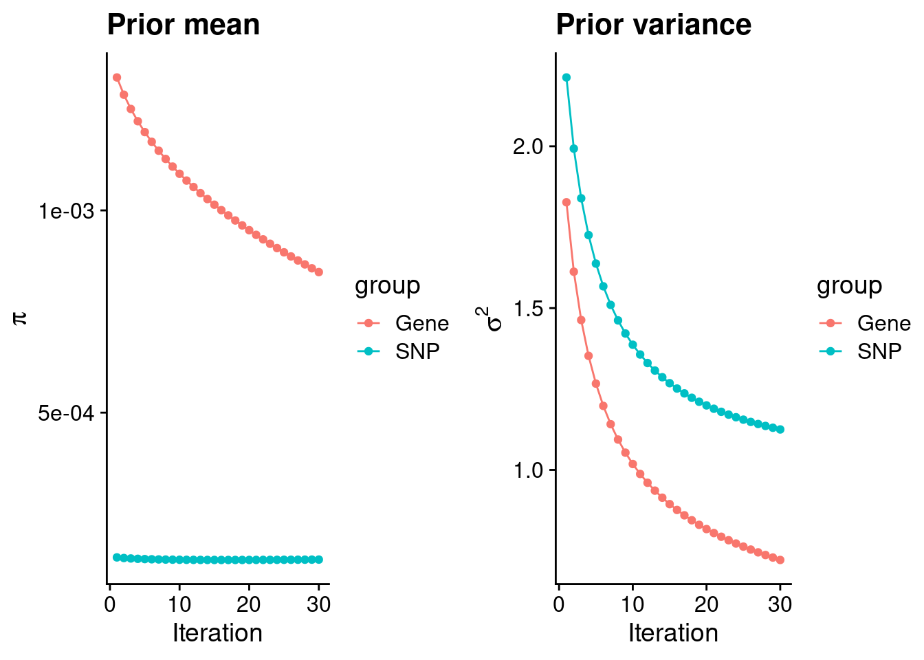
| Version | Author | Date |
|---|---|---|
| dfd2b5f | wesleycrouse | 2021-09-07 |
#estimated group prior
estimated_group_prior <- group_prior_rec[,ncol(group_prior_rec)]
names(estimated_group_prior) <- c("gene", "snp")
estimated_group_prior["snp"] <- estimated_group_prior["snp"]*thin #adjust parameter to account for thin argument
print(estimated_group_prior)
gene snp
0.0008474940 0.0001366605 #estimated group prior variance
estimated_group_prior_var <- group_prior_var_rec[,ncol(group_prior_var_rec)]
names(estimated_group_prior_var) <- c("gene", "snp")
print(estimated_group_prior_var) gene snp
0.7217176 1.1250624 #report sample size
print(sample_size)[1] 54498#report group size
group_size <- c(nrow(ctwas_gene_res), n_snps)
print(group_size)[1] 10901 8697330#estimated group PVE
estimated_group_pve <- estimated_group_prior_var*estimated_group_prior*group_size/sample_size #check PVE calculation
names(estimated_group_pve) <- c("gene", "snp")
print(estimated_group_pve) gene snp
0.000122346 0.024537192 #compare sum(PIP*mu2/sample_size) with above PVE calculation
c(sum(ctwas_gene_res$PVE),sum(ctwas_snp_res$PVE))[1] 0.002731761 0.502393806Genes with highest PIPs
#distribution of PIPs
hist(ctwas_gene_res$susie_pip, xlim=c(0,1), main="Distribution of Gene PIPs")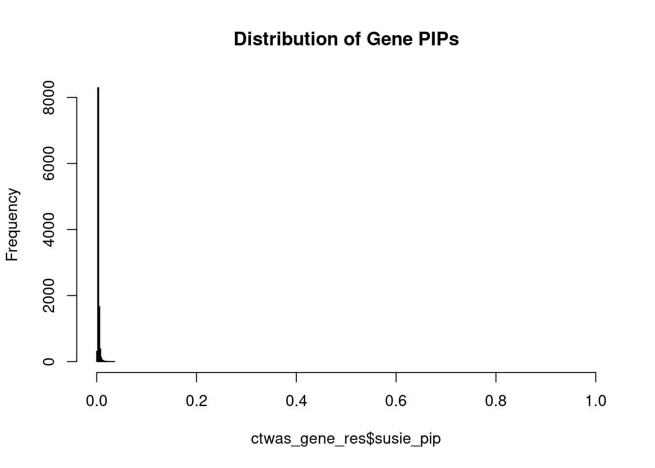
| Version | Author | Date |
|---|---|---|
| dfd2b5f | wesleycrouse | 2021-09-07 |
#genes with PIP>0.8 or 20 highest PIPs
head(ctwas_gene_res[order(-ctwas_gene_res$susie_pip),report_cols], max(sum(ctwas_gene_res$susie_pip>0.8), 20))
genename region_tag susie_pip mu2 PVE z
2518 LIN7A 12_49 0.036 12.01 7.8e-06 -3.42
5908 GTF3C5 9_70 0.035 11.71 7.6e-06 -3.35
2586 GOLT1B 12_16 0.025 11.56 5.2e-06 -3.46
4693 SETDB2 13_21 0.025 10.81 5.0e-06 3.48
8233 KCNS3 2_10 0.024 10.88 4.7e-06 3.66
11 RAD52 12_1 0.024 10.70 4.7e-06 -3.31
3991 ATP1B2 17_7 0.024 11.86 5.2e-06 -4.47
10146 MVB12B 9_65 0.022 10.32 4.2e-06 3.24
11309 C12orf75 12_63 0.022 10.24 4.2e-06 3.57
4223 DNAJB1 19_12 0.021 9.95 3.9e-06 -3.15
1006 COBLL1 2_100 0.020 9.97 3.7e-06 3.36
8238 CHCHD7 8_44 0.020 10.17 3.7e-06 3.09
5115 NUP58 13_6 0.020 9.83 3.6e-06 3.01
3881 VIL1 2_129 0.019 9.64 3.4e-06 -3.24
11478 HLA-DMB 6_27 0.019 9.08 3.1e-06 -3.05
10260 BCO2 11_66 0.019 9.81 3.4e-06 -3.12
5305 PELP1 17_4 0.019 10.25 3.6e-06 4.25
7089 IGFBP7 4_41 0.018 10.20 3.3e-06 3.13
3265 DLST 14_34 0.018 10.24 3.4e-06 -3.45
1672 TTI1 20_22 0.018 9.10 2.9e-06 -2.85Genes with largest effect sizes
#plot PIP vs effect size
plot(ctwas_gene_res$susie_pip, ctwas_gene_res$mu2, xlab="PIP", ylab="mu^2", main="Gene PIPs vs Effect Size")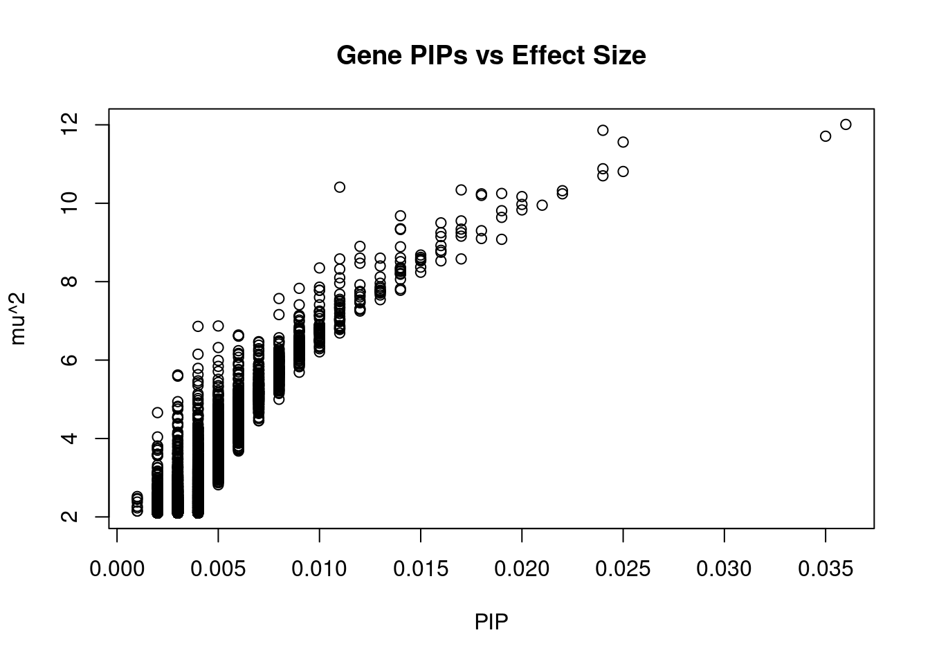
| Version | Author | Date |
|---|---|---|
| dfd2b5f | wesleycrouse | 2021-09-07 |
#genes with 20 largest effect sizes
head(ctwas_gene_res[order(-ctwas_gene_res$mu2),report_cols],20)
genename region_tag susie_pip mu2 PVE z
2518 LIN7A 12_49 0.036 12.01 7.8e-06 -3.42
3991 ATP1B2 17_7 0.024 11.86 5.2e-06 -4.47
5908 GTF3C5 9_70 0.035 11.71 7.6e-06 -3.35
2586 GOLT1B 12_16 0.025 11.56 5.2e-06 -3.46
8233 KCNS3 2_10 0.024 10.88 4.7e-06 3.66
4693 SETDB2 13_21 0.025 10.81 5.0e-06 3.48
11 RAD52 12_1 0.024 10.70 4.7e-06 -3.31
10642 HLA-C 6_25 0.011 10.41 2.2e-06 -4.52
854 EXOSC7 3_31 0.017 10.34 3.3e-06 3.54
10146 MVB12B 9_65 0.022 10.32 4.2e-06 3.24
5305 PELP1 17_4 0.019 10.25 3.6e-06 4.25
11309 C12orf75 12_63 0.022 10.24 4.2e-06 3.57
3265 DLST 14_34 0.018 10.24 3.4e-06 -3.45
7089 IGFBP7 4_41 0.018 10.20 3.3e-06 3.13
8238 CHCHD7 8_44 0.020 10.17 3.7e-06 3.09
1006 COBLL1 2_100 0.020 9.97 3.7e-06 3.36
4223 DNAJB1 19_12 0.021 9.95 3.9e-06 -3.15
5115 NUP58 13_6 0.020 9.83 3.6e-06 3.01
10260 BCO2 11_66 0.019 9.81 3.4e-06 -3.12
6880 TNFSF13 17_7 0.014 9.68 2.5e-06 4.26Genes with highest PVE
#genes with 20 highest pve
head(ctwas_gene_res[order(-ctwas_gene_res$PVE),report_cols],20)
genename region_tag susie_pip mu2 PVE z
2518 LIN7A 12_49 0.036 12.01 7.8e-06 -3.42
5908 GTF3C5 9_70 0.035 11.71 7.6e-06 -3.35
2586 GOLT1B 12_16 0.025 11.56 5.2e-06 -3.46
3991 ATP1B2 17_7 0.024 11.86 5.2e-06 -4.47
4693 SETDB2 13_21 0.025 10.81 5.0e-06 3.48
8233 KCNS3 2_10 0.024 10.88 4.7e-06 3.66
11 RAD52 12_1 0.024 10.70 4.7e-06 -3.31
10146 MVB12B 9_65 0.022 10.32 4.2e-06 3.24
11309 C12orf75 12_63 0.022 10.24 4.2e-06 3.57
4223 DNAJB1 19_12 0.021 9.95 3.9e-06 -3.15
1006 COBLL1 2_100 0.020 9.97 3.7e-06 3.36
8238 CHCHD7 8_44 0.020 10.17 3.7e-06 3.09
5115 NUP58 13_6 0.020 9.83 3.6e-06 3.01
5305 PELP1 17_4 0.019 10.25 3.6e-06 4.25
3881 VIL1 2_129 0.019 9.64 3.4e-06 -3.24
10260 BCO2 11_66 0.019 9.81 3.4e-06 -3.12
3265 DLST 14_34 0.018 10.24 3.4e-06 -3.45
854 EXOSC7 3_31 0.017 10.34 3.3e-06 3.54
7089 IGFBP7 4_41 0.018 10.20 3.3e-06 3.13
11478 HLA-DMB 6_27 0.019 9.08 3.1e-06 -3.05Genes with largest z scores
#genes with 20 largest z scores
head(ctwas_gene_res[order(-abs(ctwas_gene_res$z)),report_cols],20)
genename region_tag susie_pip mu2 PVE z
10642 HLA-C 6_25 0.011 10.41 2.2e-06 -4.52
3991 ATP1B2 17_7 0.024 11.86 5.2e-06 -4.47
6880 TNFSF13 17_7 0.014 9.68 2.5e-06 4.26
5305 PELP1 17_4 0.019 10.25 3.6e-06 4.25
5308 ARRB2 17_4 0.013 8.60 2.0e-06 -3.96
8233 KCNS3 2_10 0.024 10.88 4.7e-06 3.66
11309 C12orf75 12_63 0.022 10.24 4.2e-06 3.57
854 EXOSC7 3_31 0.017 10.34 3.3e-06 3.54
4693 SETDB2 13_21 0.025 10.81 5.0e-06 3.48
2586 GOLT1B 12_16 0.025 11.56 5.2e-06 -3.46
3265 DLST 14_34 0.018 10.24 3.4e-06 -3.45
2518 LIN7A 12_49 0.036 12.01 7.8e-06 -3.42
1410 RNF215 22_10 0.017 9.55 3.0e-06 -3.41
1006 COBLL1 2_100 0.020 9.97 3.7e-06 3.36
5908 GTF3C5 9_70 0.035 11.71 7.6e-06 -3.35
7177 CLEC3B 3_31 0.014 9.33 2.4e-06 3.33
11 RAD52 12_1 0.024 10.70 4.7e-06 -3.31
9074 TCAIM 3_31 0.011 8.32 1.7e-06 -3.29
11399 TNFSF12 17_7 0.006 6.17 7.0e-07 3.28
5643 ZNF660 3_31 0.010 7.86 1.4e-06 3.27Comparing z scores and PIPs
#set nominal signifiance threshold for z scores
alpha <- 0.05

#bonferroni adjusted threshold for z scores
sig_thresh <- qnorm(1-(alpha/nrow(ctwas_gene_res)/2), lower=T)

#Q-Q plot for z scores
obs_z <- ctwas_gene_res$z[order(ctwas_gene_res$z)]
exp_z <- qnorm((1:nrow(ctwas_gene_res))/nrow(ctwas_gene_res))

plot(exp_z, obs_z, xlab="Expected z", ylab="Observed z", main="Gene z score Q-Q plot")
abline(a=0,b=1)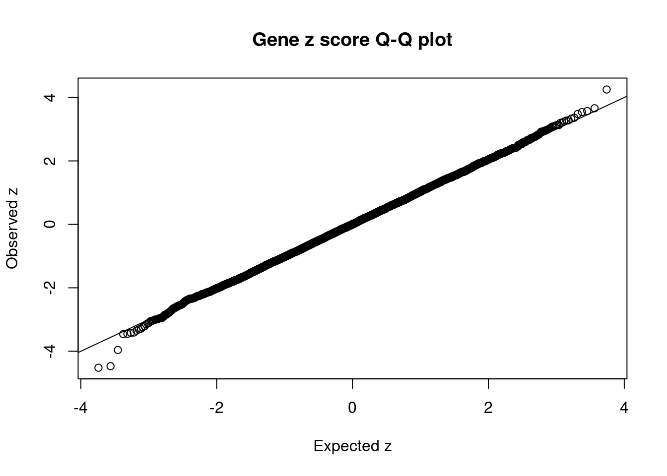
| Version | Author | Date |
|---|---|---|
| dfd2b5f | wesleycrouse | 2021-09-07 |
#plot z score vs PIP
plot(abs(ctwas_gene_res$z), ctwas_gene_res$susie_pip, xlab="abs(z)", ylab="PIP")
abline(v=sig_thresh, col="red", lty=2)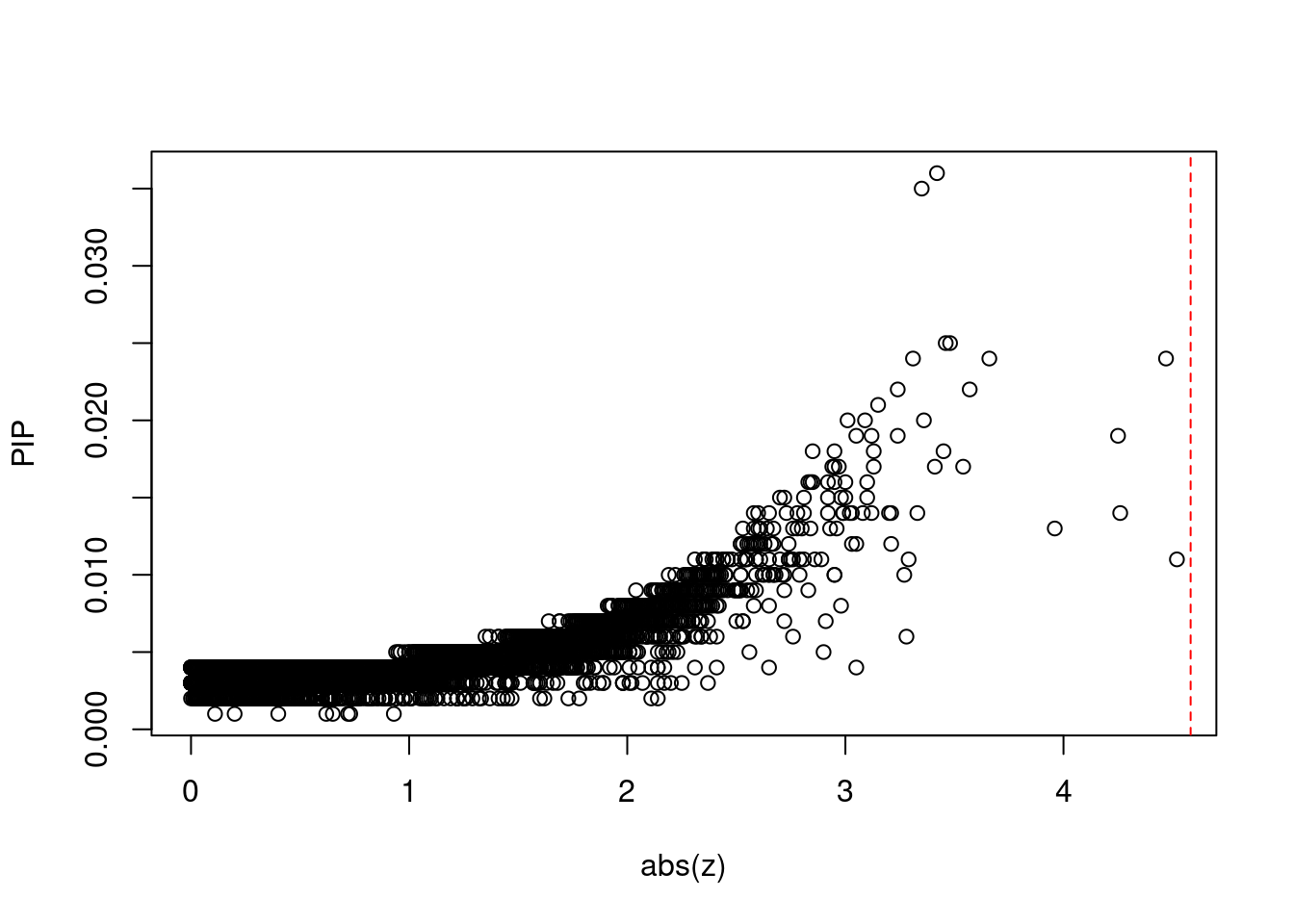
| Version | Author | Date |
|---|---|---|
| dfd2b5f | wesleycrouse | 2021-09-07 |
#proportion of significant z scores
mean(abs(ctwas_gene_res$z) > sig_thresh)
[1] 0#genes with most significant z scores
head(ctwas_gene_res[order(-abs(ctwas_gene_res$z)),report_cols],20) genename region_tag susie_pip mu2 PVE z
10642 HLA-C 6_25 0.011 10.41 2.2e-06 -4.52
3991 ATP1B2 17_7 0.024 11.86 5.2e-06 -4.47
6880 TNFSF13 17_7 0.014 9.68 2.5e-06 4.26
5305 PELP1 17_4 0.019 10.25 3.6e-06 4.25
5308 ARRB2 17_4 0.013 8.60 2.0e-06 -3.96
8233 KCNS3 2_10 0.024 10.88 4.7e-06 3.66
11309 C12orf75 12_63 0.022 10.24 4.2e-06 3.57
854 EXOSC7 3_31 0.017 10.34 3.3e-06 3.54
4693 SETDB2 13_21 0.025 10.81 5.0e-06 3.48
2586 GOLT1B 12_16 0.025 11.56 5.2e-06 -3.46
3265 DLST 14_34 0.018 10.24 3.4e-06 -3.45
2518 LIN7A 12_49 0.036 12.01 7.8e-06 -3.42
1410 RNF215 22_10 0.017 9.55 3.0e-06 -3.41
1006 COBLL1 2_100 0.020 9.97 3.7e-06 3.36
5908 GTF3C5 9_70 0.035 11.71 7.6e-06 -3.35
7177 CLEC3B 3_31 0.014 9.33 2.4e-06 3.33
11 RAD52 12_1 0.024 10.70 4.7e-06 -3.31
9074 TCAIM 3_31 0.011 8.32 1.7e-06 -3.29
11399 TNFSF12 17_7 0.006 6.17 7.0e-07 3.28
5643 ZNF660 3_31 0.010 7.86 1.4e-06 3.27Locus plots for genes and SNPs
ctwas_gene_res_sortz <- ctwas_gene_res[order(-abs(ctwas_gene_res$z)),]

n_plots <- 5
for (region_tag_plot in head(unique(ctwas_gene_res_sortz$region_tag), n_plots)){
  ctwas_res_region <-  ctwas_res[ctwas_res$region_tag==region_tag_plot,]
  start <- min(ctwas_res_region$pos)
  end <- max(ctwas_res_region$pos)

  ctwas_res_region <- ctwas_res_region[order(ctwas_res_region$pos),]
  ctwas_res_region_gene <- ctwas_res_region[ctwas_res_region$type=="gene",]
  ctwas_res_region_snp <- ctwas_res_region[ctwas_res_region$type=="SNP",]

  #region name
  print(paste0("Region: ", region_tag_plot))

  #table of genes in region
  print(ctwas_res_region_gene[,report_cols])

  par(mfrow=c(4,1))

  #gene z scores
  plot(ctwas_res_region_gene$pos, abs(ctwas_res_region_gene$z), xlab="Position", ylab="abs(gene_z)", xlim=c(start,end),
   ylim=c(0,max(sig_thresh, abs(ctwas_res_region_gene$z))),
   main=paste0("Region: ", region_tag_plot))
  abline(h=sig_thresh,col="red",lty=2)

  #significance threshold for SNPs
  alpha_snp <- 5*10^(-8)
  sig_thresh_snp <- qnorm(1-alpha_snp/2, lower=T)

  #snp z scores
  plot(ctwas_res_region_snp$pos, abs(ctwas_res_region_snp$z), xlab="Position", ylab="abs(snp_z)",xlim=c(start,end),
   ylim=c(0,max(sig_thresh_snp, max(abs(ctwas_res_region_snp$z)))))
  abline(h=sig_thresh_snp,col="purple",lty=2)

  #gene pips
  plot(ctwas_res_region_gene$pos, ctwas_res_region_gene$susie_pip, xlab="Position", ylab="Gene PIP", xlim=c(start,end), ylim=c(0,1))
  abline(h=0.8,col="blue",lty=2)

  #snp pips
  plot(ctwas_res_region_snp$pos, ctwas_res_region_snp$susie_pip, xlab="Position", ylab="SNP PIP", xlim=c(start,end), ylim=c(0,1))
  abline(h=0.8,col="blue",lty=2)
}
[1] "Region: 6_25"
genename region_tag susie_pip mu2 PVE z
10653 DDR1 6_25 0.002 2.26 6.7e-08 0.28
4838 VARS2 6_25 0.003 4.38 2.2e-07 2.25
10854 GTF2H4 6_25 0.003 4.57 2.4e-07 -2.17
10044 SFTA2 6_25 0.002 2.31 7.0e-08 -0.97
10646 PSORS1C1 6_25 0.002 3.81 1.6e-07 2.11
10645 PSORS1C2 6_25 0.002 2.11 6.0e-08 -0.32
11297 HLA-B 6_25 0.002 2.10 6.0e-08 -0.08
4832 TCF19 6_25 0.002 2.16 6.3e-08 -0.31
10644 CCHCR1 6_25 0.002 2.16 6.3e-08 -0.31
10643 POU5F1 6_25 0.002 2.79 9.4e-08 -1.22
10771 HCG27 6_25 0.004 6.15 4.6e-07 3.05
10642 HLA-C 6_25 0.011 10.41 2.2e-06 -4.52
12306 XXbac-BPG181B23.7 6_25 0.002 2.95 1.0e-07 -1.22
10640 MICA 6_25 0.002 2.98 1.1e-07 1.78
10639 MICB 6_25 0.002 2.43 7.5e-08 -0.54
10417 DDX39B 6_25 0.002 3.57 1.5e-07 1.29
10637 NFKBIL1 6_25 0.002 2.13 6.1e-08 0.13
10852 ATP6V1G2 6_25 0.002 2.10 6.0e-08 -0.02
11110 LTA 6_25 0.002 2.26 6.7e-08 -0.54
11237 TNF 6_25 0.002 3.07 1.1e-07 -1.09
10635 NCR3 6_25 0.002 3.32 1.3e-07 1.45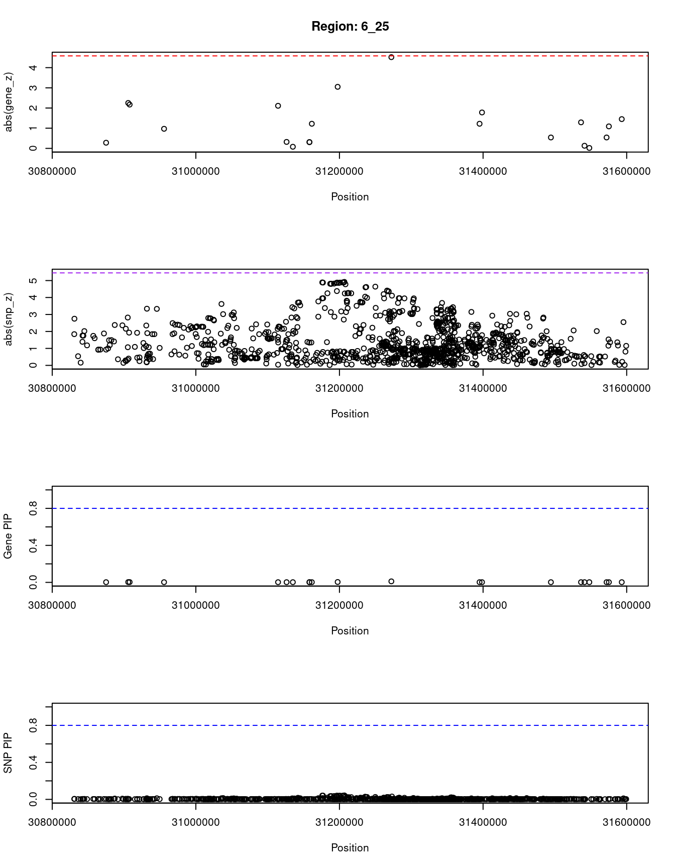
| Version | Author | Date |
|---|---|---|
| dfd2b5f | wesleycrouse | 2021-09-07 |
[1] "Region: 17_7"
          genename region_tag susie_pip   mu2     PVE     z
9229       TMEM102       17_7     0.003  2.47 1.2e-07 -1.04
6882         FGF11       17_7     0.009  7.83 1.3e-06  2.59
11885      SLC35G6       17_7     0.002  2.32 1.0e-07  0.82
11399      TNFSF12       17_7     0.006  6.17 7.0e-07  3.28
6880       TNFSF13       17_7     0.014  9.68 2.5e-06  4.26
6881         SENP3       17_7     0.003  2.68 1.3e-07 -0.61
6883        EIF4A1       17_7     0.002  2.32 1.0e-07 -1.05
5313          SAT2       17_7     0.002  2.10 9.0e-08 -0.13
3991        ATP1B2       17_7     0.024 11.86 5.2e-06 -4.47
5311        WRAP53       17_7     0.004  4.76 3.8e-07 -2.14
9477         DNAH2       17_7     0.006  5.76 5.9e-07  2.76
7853        TMEM88       17_7     0.003  2.55 1.2e-07  0.85
9115    AC025335.1       17_7     0.003  2.63 1.3e-07  0.90
8143        KCNAB3       17_7     0.002  2.17 9.4e-08 -0.34
8142        CNTROB       17_7     0.002  2.23 9.9e-08 -0.44
10982        VAMP2       17_7     0.003  2.92 1.5e-07  0.99
9063       TMEM107       17_7     0.003  3.01 1.6e-07 -1.01
9059         AURKB       17_7     0.002  2.12 9.1e-08  0.17
9053          CTC1       17_7     0.002  2.11 9.0e-08  0.13
9046          PFAS       17_7     0.011  8.58 1.7e-06  2.75
12191 RP11-849F2.9       17_7     0.002  2.22 9.7e-08 -0.32
3703      SLC25A35       17_7     0.002  2.14 9.2e-08  0.21
9538         KRBA2       17_7     0.002  2.17 9.4e-08 -0.33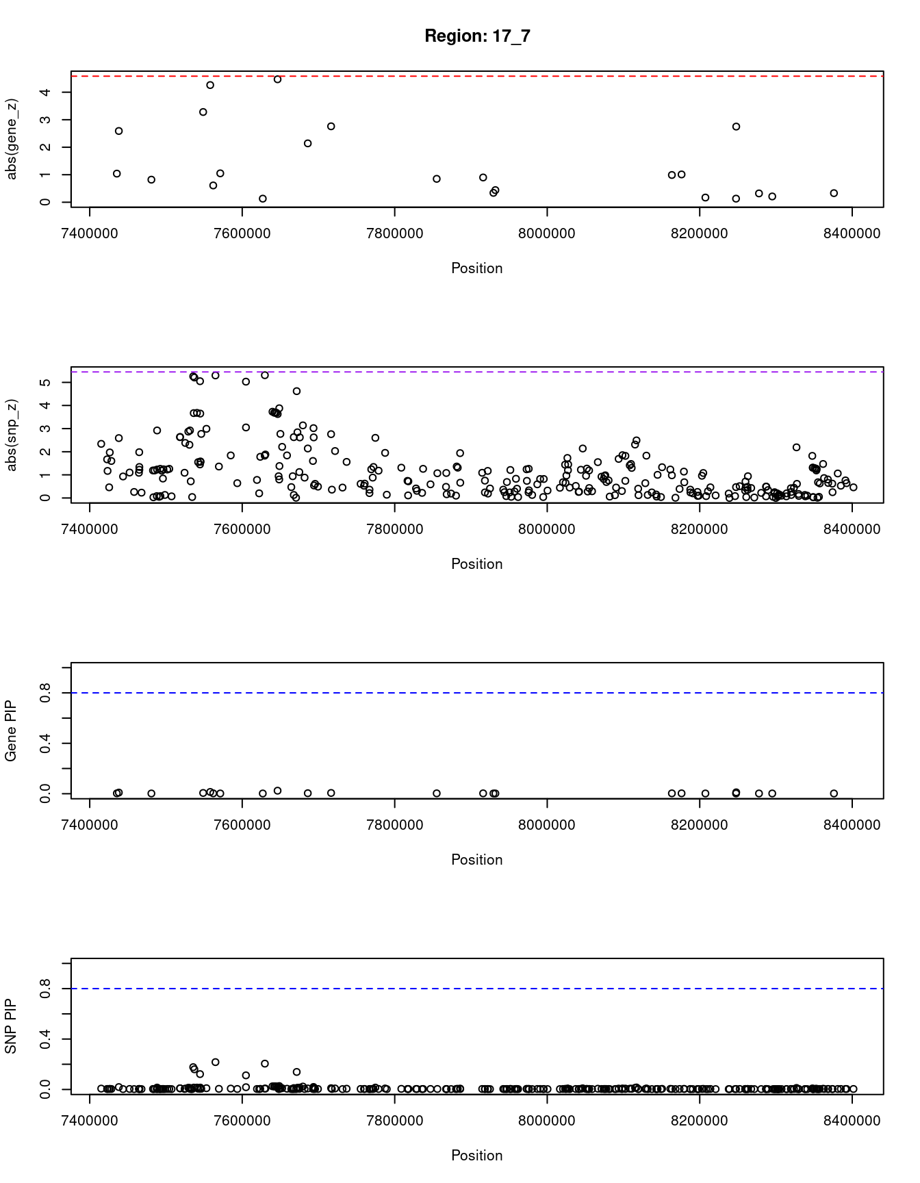
| Version | Author | Date |
|---|---|---|
| dfd2b5f | wesleycrouse | 2021-09-07 |
[1] "Region: 17_4"
     genename region_tag susie_pip   mu2     PVE     z
1024    ITGAE       17_4     0.006  5.36 5.8e-07  1.93
811    ATP2A3       17_4     0.005  4.76 4.5e-07  1.86
819     ZZEF1       17_4     0.003  2.10 1.0e-07 -0.02
4260   UBE2G1       17_4     0.004  3.50 2.4e-07  1.32
9334    SPNS3       17_4     0.003  2.12 1.1e-07  0.14
7828     GGT6       17_4     0.003  2.25 1.2e-07  0.33
4257  MYBBP1A       17_4     0.003  2.26 1.2e-07 -0.73
5305    PELP1       17_4     0.019 10.25 3.6e-06  4.25
5308    ARRB2       17_4     0.013  8.60 2.0e-06 -3.96
6876    MED11       17_4     0.003  2.29 1.2e-07  0.63
5310  ZMYND15       17_4     0.004  3.40 2.3e-07 -1.06
9363     VMO1       17_4     0.005  4.93 4.8e-07 -1.99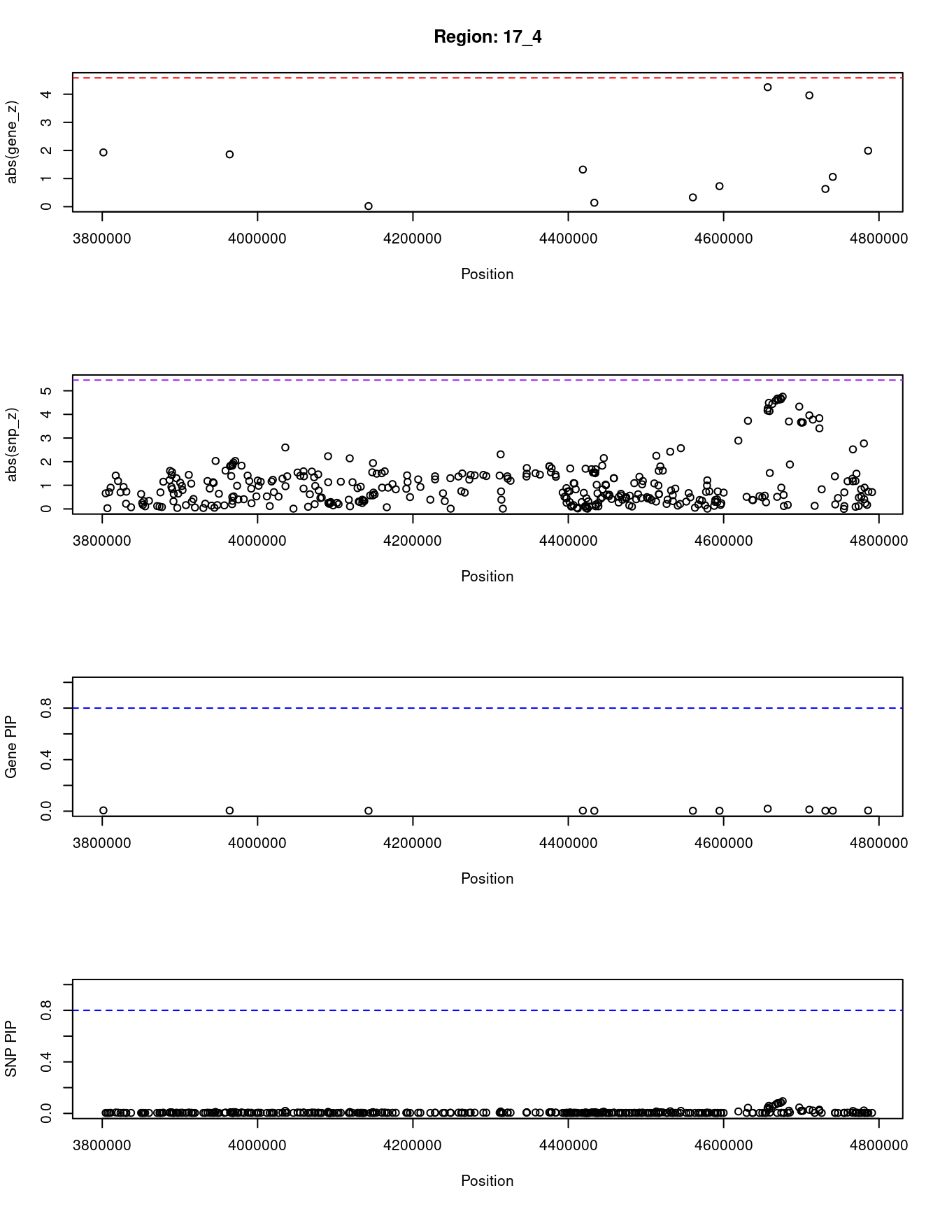
| Version | Author | Date |
|---|---|---|
| dfd2b5f | wesleycrouse | 2021-09-07 |
[1] "Region: 2_10"
      genename region_tag susie_pip   mu2     PVE     z
10301   FAM49A       2_10     0.003  2.26 1.3e-07  0.45
10925 RAD51AP2       2_10     0.005  3.92 3.3e-07  1.60
7032     VSNL1       2_10     0.003  2.76 1.7e-07  0.92
8996      GEN1       2_10     0.003  2.61 1.6e-07 -0.94
7031      SMC6       2_10     0.004  3.20 2.3e-07  1.31
8233     KCNS3       2_10     0.024 10.88 4.7e-06  3.66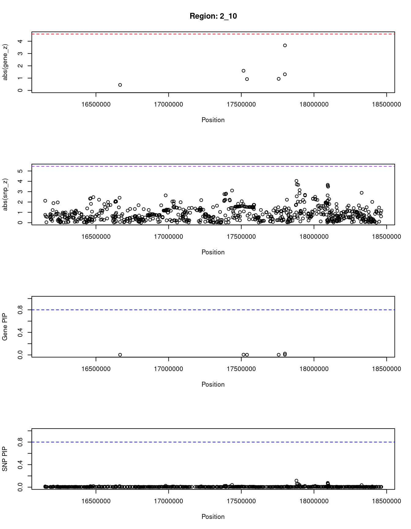
| Version | Author | Date |
|---|---|---|
| dfd2b5f | wesleycrouse | 2021-09-07 |
[1] "Region: 12_63"
      genename region_tag susie_pip   mu2     PVE    z
4676   SLC41A2      12_63     0.004  2.69 1.8e-07 0.79
6082  C12orf45      12_63     0.003  2.15 1.3e-07 0.28
4675    WASHC4      12_63     0.005  3.53 3.0e-07 1.45
11309 C12orf75      12_63     0.022 10.24 4.2e-06 3.57
4672     APPL2      12_63     0.005  3.59 3.0e-07 1.52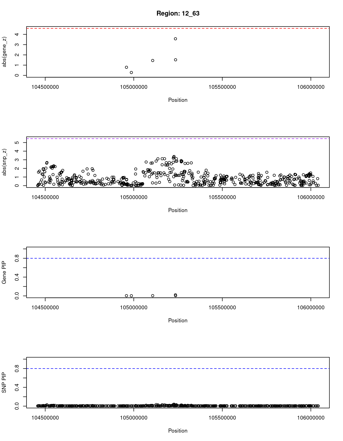
| Version | Author | Date |
|---|---|---|
| dfd2b5f | wesleycrouse | 2021-09-07 |
SNPs with highest PIPs
#snps with PIP>0.8 or 20 highest PIPs
head(ctwas_snp_res[order(-ctwas_snp_res$susie_pip),report_cols_snps],
max(sum(ctwas_snp_res$susie_pip>0.8), 20))
id region_tag susie_pip mu2 PVE z
140037 rs75620930 3_1 0.242 23.92 1.1e-04 4.34
396298 rs62444120 7_28 0.242 23.84 1.1e-04 -4.35
476904 rs112371525 8_89 0.219 23.32 9.4e-05 4.23
761470 rs4968212 17_7 0.217 25.19 1.0e-04 -5.30
761480 rs62059839 17_7 0.205 24.86 9.4e-05 5.31
679108 rs1959607 14_1 0.202 22.92 8.5e-05 4.21
526099 rs551737161 10_16 0.187 24.22 8.3e-05 3.60
813811 rs73000658 19_16 0.184 22.18 7.5e-05 -4.06
761458 rs9892862 17_7 0.177 23.99 7.8e-05 5.26
319306 rs13160700 5_104 0.175 22.38 7.2e-05 -4.06
165332 rs9813399 3_53 0.174 21.67 6.9e-05 4.14
806869 rs117700303 19_2 0.170 22.08 6.9e-05 -4.07
70306 rs13429539 2_7 0.167 22.83 7.0e-05 -4.12
513886 rs10760461 9_65 0.167 22.03 6.8e-05 4.10
417774 rs876169 7_68 0.161 21.86 6.5e-05 4.31
272419 rs112157462 5_14 0.160 21.39 6.3e-05 3.98
761460 rs8073177 17_7 0.160 23.44 6.9e-05 5.21
154020 rs76750610 3_28 0.155 21.22 6.0e-05 -3.93
459963 rs553564201 8_57 0.155 22.03 6.3e-05 3.99
381048 rs113784847 7_1 0.151 21.78 6.0e-05 -4.04SNPs with largest effect sizes
#plot PIP vs effect size
plot(ctwas_snp_res$susie_pip, ctwas_snp_res$mu2, xlab="PIP", ylab="mu^2", main="SNP PIPs vs Effect Size")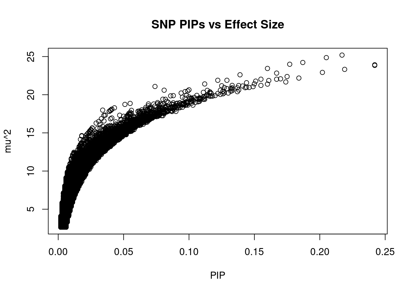
| Version | Author | Date |
|---|---|---|
| dfd2b5f | wesleycrouse | 2021-09-07 |
#SNPs with 50 largest effect sizes
head(ctwas_snp_res[order(-ctwas_snp_res$mu2),report_cols_snps],50)
id region_tag susie_pip mu2 PVE z
761470 rs4968212 17_7 0.217 25.19 1.0e-04 -5.30
761480 rs62059839 17_7 0.205 24.86 9.4e-05 5.31
526099 rs551737161 10_16 0.187 24.22 8.3e-05 3.60
761458 rs9892862 17_7 0.177 23.99 7.8e-05 5.26
140037 rs75620930 3_1 0.242 23.92 1.1e-04 4.34
396298 rs62444120 7_28 0.242 23.84 1.1e-04 -4.35
761460 rs8073177 17_7 0.160 23.44 6.9e-05 5.21
476904 rs112371525 8_89 0.219 23.32 9.4e-05 4.23
679108 rs1959607 14_1 0.202 22.92 8.5e-05 4.21
70306 rs13429539 2_7 0.167 22.83 7.0e-05 -4.12
761500 rs1641549 17_7 0.139 22.61 5.7e-05 -4.62
319306 rs13160700 5_104 0.175 22.38 7.2e-05 -4.06
813811 rs73000658 19_16 0.184 22.18 7.5e-05 -4.06
806869 rs117700303 19_2 0.170 22.08 6.9e-05 -4.07
459963 rs553564201 8_57 0.155 22.03 6.3e-05 3.99
513886 rs10760461 9_65 0.167 22.03 6.8e-05 4.10
39473 rs192164271 1_80 0.129 21.89 5.2e-05 3.94
761464 rs11078694 17_7 0.122 21.89 4.9e-05 -5.05
417774 rs876169 7_68 0.161 21.86 6.5e-05 4.31
381048 rs113784847 7_1 0.151 21.78 6.0e-05 -4.04
165332 rs9813399 3_53 0.174 21.67 6.9e-05 4.14
327669 rs192338591 6_13 0.144 21.57 5.7e-05 3.94
138489 rs3791461 2_142 0.150 21.42 5.9e-05 -3.97
761474 rs149932962 17_7 0.112 21.41 4.4e-05 5.03
272419 rs112157462 5_14 0.160 21.39 6.3e-05 3.98
96986 rs187600283 2_58 0.133 21.22 5.2e-05 3.88
154020 rs76750610 3_28 0.155 21.22 6.0e-05 -3.93
742136 rs143894776 16_23 0.138 21.20 5.4e-05 -3.90
642695 rs146568110 12_75 0.125 21.17 4.9e-05 3.84
423042 rs9640863 7_80 0.141 21.14 5.5e-05 -3.96
238187 rs142227684 4_72 0.074 21.08 2.9e-05 3.79
2845 rs2274332 1_6 0.149 21.06 5.8e-05 -3.89
106803 rs62162215 2_78 0.144 20.98 5.5e-05 -3.94
598854 rs73008432 11_70 0.146 20.95 5.6e-05 4.04
182446 rs9823043 3_85 0.127 20.94 4.9e-05 -4.05
64719 rs79505543 1_129 0.143 20.92 5.5e-05 3.85
710597 rs76553406 15_9 0.133 20.91 5.1e-05 3.91
582710 rs140333597 11_37 0.137 20.90 5.2e-05 3.86
819786 rs544367902 19_27 0.132 20.82 5.0e-05 3.82
368002 rs148062999 6_88 0.129 20.80 4.9e-05 3.84
763904 rs58335060 17_13 0.133 20.74 5.1e-05 -4.13
199766 rs115771219 3_119 0.100 20.64 3.8e-05 -3.74
24562 rs41284595 1_52 0.138 20.62 5.2e-05 -3.85
468856 rs149885805 8_74 0.124 20.59 4.7e-05 -3.82
611212 rs7308471 12_15 0.081 20.59 3.1e-05 3.96
394648 rs11371390 7_26 0.114 20.57 4.3e-05 -4.04
56411 rs78763889 1_111 0.133 20.53 5.0e-05 -4.03
382126 rs10951073 7_5 0.099 20.49 3.7e-05 -3.93
257296 rs13121691 4_110 0.126 20.47 4.7e-05 -3.84
645510 rs1696452 12_80 0.132 20.46 5.0e-05 3.78SNPs with highest PVE
#SNPs with 50 highest pve
head(ctwas_snp_res[order(-ctwas_snp_res$PVE),report_cols_snps],50)
id region_tag susie_pip mu2 PVE z
140037 rs75620930 3_1 0.242 23.92 1.1e-04 4.34
396298 rs62444120 7_28 0.242 23.84 1.1e-04 -4.35
761470 rs4968212 17_7 0.217 25.19 1.0e-04 -5.30
476904 rs112371525 8_89 0.219 23.32 9.4e-05 4.23
761480 rs62059839 17_7 0.205 24.86 9.4e-05 5.31
679108 rs1959607 14_1 0.202 22.92 8.5e-05 4.21
526099 rs551737161 10_16 0.187 24.22 8.3e-05 3.60
761458 rs9892862 17_7 0.177 23.99 7.8e-05 5.26
813811 rs73000658 19_16 0.184 22.18 7.5e-05 -4.06
319306 rs13160700 5_104 0.175 22.38 7.2e-05 -4.06
70306 rs13429539 2_7 0.167 22.83 7.0e-05 -4.12
165332 rs9813399 3_53 0.174 21.67 6.9e-05 4.14
761460 rs8073177 17_7 0.160 23.44 6.9e-05 5.21
806869 rs117700303 19_2 0.170 22.08 6.9e-05 -4.07
513886 rs10760461 9_65 0.167 22.03 6.8e-05 4.10
417774 rs876169 7_68 0.161 21.86 6.5e-05 4.31
272419 rs112157462 5_14 0.160 21.39 6.3e-05 3.98
459963 rs553564201 8_57 0.155 22.03 6.3e-05 3.99
154020 rs76750610 3_28 0.155 21.22 6.0e-05 -3.93
381048 rs113784847 7_1 0.151 21.78 6.0e-05 -4.04
138489 rs3791461 2_142 0.150 21.42 5.9e-05 -3.97
2845 rs2274332 1_6 0.149 21.06 5.8e-05 -3.89
327669 rs192338591 6_13 0.144 21.57 5.7e-05 3.94
761500 rs1641549 17_7 0.139 22.61 5.7e-05 -4.62
598854 rs73008432 11_70 0.146 20.95 5.6e-05 4.04
64719 rs79505543 1_129 0.143 20.92 5.5e-05 3.85
106803 rs62162215 2_78 0.144 20.98 5.5e-05 -3.94
423042 rs9640863 7_80 0.141 21.14 5.5e-05 -3.96
742136 rs143894776 16_23 0.138 21.20 5.4e-05 -3.90
24562 rs41284595 1_52 0.138 20.62 5.2e-05 -3.85
39473 rs192164271 1_80 0.129 21.89 5.2e-05 3.94
96986 rs187600283 2_58 0.133 21.22 5.2e-05 3.88
582710 rs140333597 11_37 0.137 20.90 5.2e-05 3.86
351728 rs78874260 6_54 0.137 20.40 5.1e-05 -3.79
710597 rs76553406 15_9 0.133 20.91 5.1e-05 3.91
763904 rs58335060 17_13 0.133 20.74 5.1e-05 -4.13
56411 rs78763889 1_111 0.133 20.53 5.0e-05 -4.03
645510 rs1696452 12_80 0.132 20.46 5.0e-05 3.78
819786 rs544367902 19_27 0.132 20.82 5.0e-05 3.82
182446 rs9823043 3_85 0.127 20.94 4.9e-05 -4.05
368002 rs148062999 6_88 0.129 20.80 4.9e-05 3.84
642695 rs146568110 12_75 0.125 21.17 4.9e-05 3.84
761464 rs11078694 17_7 0.122 21.89 4.9e-05 -5.05
764807 rs139270577 17_15 0.130 20.22 4.8e-05 -3.76
99704 rs3113783 2_65 0.126 20.12 4.7e-05 -3.99
257296 rs13121691 4_110 0.126 20.47 4.7e-05 -3.84
362887 rs2350814 6_76 0.127 20.25 4.7e-05 3.91
468856 rs149885805 8_74 0.124 20.59 4.7e-05 -3.82
758122 rs11076740 16_53 0.126 20.41 4.7e-05 -3.98
685436 rs117875427 14_11 0.124 20.04 4.6e-05 -3.85SNPs with largest z scores
#SNPs with 50 largest z scores
head(ctwas_snp_res[order(-abs(ctwas_snp_res$z)),report_cols_snps],50)
id region_tag susie_pip mu2 PVE z
761480 rs62059839 17_7 0.205 24.86 9.4e-05 5.31
761470 rs4968212 17_7 0.217 25.19 1.0e-04 -5.30
761458 rs9892862 17_7 0.177 23.99 7.8e-05 5.26
761460 rs8073177 17_7 0.160 23.44 6.9e-05 5.21
761464 rs11078694 17_7 0.122 21.89 4.9e-05 -5.05
761474 rs149932962 17_7 0.112 21.41 4.4e-05 5.03
333973 rs6913470 6_25 0.043 18.28 1.4e-05 4.92
333928 rs915660 6_25 0.041 18.11 1.4e-05 4.89
333967 rs7453202 6_25 0.040 17.98 1.3e-05 4.89
333971 rs6907451 6_25 0.040 17.93 1.3e-05 4.89
333930 rs9357109 6_25 0.041 18.08 1.4e-05 4.88
333957 rs28360066 6_25 0.040 17.94 1.3e-05 4.88
333964 rs9380223 6_25 0.040 17.92 1.3e-05 4.88
333953 rs9391819 6_25 0.039 17.82 1.3e-05 4.86
333960 rs9404983 6_25 0.039 17.81 1.3e-05 4.86
333947 rs28360062 6_25 0.036 17.33 1.1e-05 4.82
333938 rs6899875 6_25 0.035 17.29 1.1e-05 4.81
333940 rs9357115 6_25 0.035 17.28 1.1e-05 4.81
333942 rs9378115 6_25 0.035 17.30 1.1e-05 4.81
333976 rs17191237 6_25 0.033 16.86 1.0e-05 4.78
760375 rs55884013 17_4 0.095 19.67 3.4e-05 -4.75
760372 rs55677157 17_4 0.084 19.01 2.9e-05 -4.69
760370 rs142108572 17_4 0.079 18.68 2.7e-05 -4.67
334039 rs28749561 6_25 0.026 15.61 7.4e-06 4.64
760373 rs11658808 17_4 0.084 19.01 2.9e-05 4.64
334022 rs28397294 6_25 0.025 15.42 7.1e-06 4.62
760371 rs2174830 17_4 0.080 18.78 2.8e-05 4.62
761500 rs1641549 17_7 0.139 22.61 5.7e-05 -4.62
334019 rs7745906 6_25 0.025 15.32 6.9e-06 4.60
760368 rs9904358 17_4 0.069 17.91 2.3e-05 4.58
760364 rs55780247 17_4 0.059 17.09 1.9e-05 -4.49
760367 rs4538065 17_4 0.055 16.66 1.7e-05 4.44
334078 rs35556213 6_25 0.025 15.37 7.0e-06 4.41
334079 rs35303934 6_25 0.024 15.23 6.7e-06 4.39
333956 rs28749557 6_25 0.021 14.62 5.8e-06 4.38
334087 rs35482069 6_25 0.023 15.00 6.4e-06 4.36
334088 rs34247821 6_25 0.023 14.98 6.3e-06 4.36
396298 rs62444120 7_28 0.242 23.84 1.1e-04 -4.35
140037 rs75620930 3_1 0.242 23.92 1.1e-04 4.34
760381 rs55999196 17_4 0.046 15.79 1.3e-05 -4.33
417774 rs876169 7_68 0.161 21.86 6.5e-05 4.31
572473 rs11031033 11_21 0.083 18.52 2.8e-05 -4.30
572475 rs10835646 11_21 0.082 18.44 2.8e-05 -4.30
333985 rs10947149 6_25 0.018 13.72 4.6e-06 4.27
155047 rs13092460 3_31 0.082 19.40 2.9e-05 -4.26
333986 rs9263947 6_25 0.024 15.18 6.6e-06 4.26
333935 rs9468882 6_25 0.019 13.95 4.9e-06 4.25
333983 rs34480332 6_25 0.018 13.63 4.5e-06 4.25
333988 rs3869109 6_25 0.024 15.13 6.6e-06 4.25
760363 rs12941694 17_4 0.045 15.66 1.3e-05 4.25Gene set enrichment for genes with PIP>0.8
#GO enrichment analysis
library(enrichR)
Welcome to enrichR
Checking connection ... Enrichr ... Connection is Live!
FlyEnrichr ... Connection is available!
WormEnrichr ... Connection is available!
YeastEnrichr ... Connection is available!
FishEnrichr ... Connection is available!dbs <- c("GO_Biological_Process_2021", "GO_Cellular_Component_2021", "GO_Molecular_Function_2021")
genes <- ctwas_gene_res$genename[ctwas_gene_res$susie_pip>0.8]
#number of genes for gene set enrichment
length(genes)[1] 0if (length(genes)>0){
GO_enrichment <- enrichr(genes, dbs)
for (db in dbs){
print(db)
df <- GO_enrichment[[db]]
df <- df[df$Adjusted.P.value<0.05,c("Term", "Overlap", "Adjusted.P.value", "Genes")]
print(df)
}
#DisGeNET enrichment
# devtools::install_bitbucket("ibi_group/disgenet2r")
library(disgenet2r)
disgenet_api_key <- get_disgenet_api_key(
email = "wesleycrouse@gmail.com",
password = "uchicago1" )
Sys.setenv(DISGENET_API_KEY= disgenet_api_key)
res_enrich <-disease_enrichment(entities=genes, vocabulary = "HGNC",
database = "CURATED" )
df <- res_enrich@qresult[1:10, c("Description", "FDR", "Ratio", "BgRatio")]
print(df)
#WebGestalt enrichment
library(WebGestaltR)
background <- ctwas_gene_res$genename
#listGeneSet()
databases <- c("pathway_KEGG", "disease_GLAD4U", "disease_OMIM")
enrichResult <- WebGestaltR(enrichMethod="ORA", organism="hsapiens",
interestGene=genes, referenceGene=background,
enrichDatabase=databases, interestGeneType="genesymbol",
referenceGeneType="genesymbol", isOutput=F)
print(enrichResult[,c("description", "size", "overlap", "FDR", "database", "userId")])
}
sessionInfo()R version 3.6.1 (2019-07-05)
Platform: x86_64-pc-linux-gnu (64-bit)
Running under: Scientific Linux 7.4 (Nitrogen)
Matrix products: default
BLAS/LAPACK: /software/openblas-0.2.19-el7-x86_64/lib/libopenblas_haswellp-r0.2.19.so
locale:
[1] LC_CTYPE=en_US.UTF-8 LC_NUMERIC=C
[3] LC_TIME=en_US.UTF-8 LC_COLLATE=en_US.UTF-8
[5] LC_MONETARY=en_US.UTF-8 LC_MESSAGES=en_US.UTF-8
[7] LC_PAPER=en_US.UTF-8 LC_NAME=C
[9] LC_ADDRESS=C LC_TELEPHONE=C
[11] LC_MEASUREMENT=en_US.UTF-8 LC_IDENTIFICATION=C
attached base packages:
[1] stats graphics grDevices utils datasets methods base
other attached packages:
[1] enrichR_3.0 cowplot_1.0.0 ggplot2_3.3.3
loaded via a namespace (and not attached):
[1] Biobase_2.44.0 httr_1.4.1
[3] bit64_4.0.5 assertthat_0.2.1
[5] stats4_3.6.1 blob_1.2.1
[7] BSgenome_1.52.0 GenomeInfoDbData_1.2.1
[9] Rsamtools_2.0.0 yaml_2.2.0
[11] progress_1.2.2 pillar_1.6.1
[13] RSQLite_2.2.7 lattice_0.20-38
[15] glue_1.4.2 digest_0.6.20
[17] GenomicRanges_1.36.0 promises_1.0.1
[19] XVector_0.24.0 colorspace_1.4-1
[21] htmltools_0.3.6 httpuv_1.5.1
[23] Matrix_1.2-18 XML_3.98-1.20
[25] pkgconfig_2.0.3 biomaRt_2.40.1
[27] zlibbioc_1.30.0 purrr_0.3.4
[29] scales_1.1.0 whisker_0.3-2
[31] later_0.8.0 BiocParallel_1.18.0
[33] git2r_0.26.1 tibble_3.1.2
[35] farver_2.1.0 generics_0.0.2
[37] IRanges_2.18.1 ellipsis_0.3.2
[39] withr_2.4.1 cachem_1.0.5
[41] SummarizedExperiment_1.14.1 GenomicFeatures_1.36.3
[43] BiocGenerics_0.30.0 magrittr_2.0.1
[45] crayon_1.4.1 memoise_2.0.0
[47] evaluate_0.14 fs_1.3.1
[49] fansi_0.5.0 tools_3.6.1
[51] data.table_1.14.0 prettyunits_1.0.2
[53] hms_1.1.0 lifecycle_1.0.0
[55] matrixStats_0.57.0 stringr_1.4.0
[57] S4Vectors_0.22.1 munsell_0.5.0
[59] DelayedArray_0.10.0 AnnotationDbi_1.46.0
[61] Biostrings_2.52.0 compiler_3.6.1
[63] GenomeInfoDb_1.20.0 rlang_0.4.11
[65] grid_3.6.1 RCurl_1.98-1.1
[67] rjson_0.2.20 VariantAnnotation_1.30.1
[69] labeling_0.3 bitops_1.0-6
[71] rmarkdown_1.13 gtable_0.3.0
[73] curl_3.3 DBI_1.1.1
[75] R6_2.5.0 GenomicAlignments_1.20.1
[77] dplyr_1.0.7 knitr_1.23
[79] rtracklayer_1.44.0 utf8_1.2.1
[81] fastmap_1.1.0 bit_4.0.4
[83] workflowr_1.6.2 rprojroot_2.0.2
[85] stringi_1.4.3 parallel_3.6.1
[87] Rcpp_1.0.6 vctrs_0.3.8
[89] tidyselect_1.1.0 xfun_0.8