Lipoprotein A (quantile)

Last updated: 2021-09-09

Checks: 6 1

Knit directory: ctwas_applied/

This reproducible R Markdown analysis was created with workflowr (version 1.6.2). The Checks tab describes the reproducibility checks that were applied when the results were created. The Past versions tab lists the development history.

R Markdown file: uncommitted changes

The R Markdown file has unstaged changes. To know which version of the R Markdown file created these results, you’ll want to first commit it to the Git repo. If you’re still working on the analysis, you can ignore this warning. When you’re finished, you can run wflow_publish to commit the R Markdown file and build the HTML.

Environment: empty

Great job! The global environment was empty. Objects defined in the global environment can affect the analysis in your R Markdown file in unknown ways. For reproduciblity it’s best to always run the code in an empty environment.

Seed: set.seed(20210726)

The command set.seed(20210726) was run prior to running the code in the R Markdown file. Setting a seed ensures that any results that rely on randomness, e.g. subsampling or permutations, are reproducible.

Session information: recorded

Great job! Recording the operating system, R version, and package versions is critical for reproducibility.

Cache: none

Nice! There were no cached chunks for this analysis, so you can be confident that you successfully produced the results during this run.

File paths: relative

Great job! Using relative paths to the files within your workflowr project makes it easier to run your code on other machines.

Repository version: 59e5f4d

Great! You are using Git for version control. Tracking code development and connecting the code version to the results is critical for reproducibility.

The results in this page were generated with repository version 59e5f4d. See the Past versions tab to see a history of the changes made to the R Markdown and HTML files.

Note that you need to be careful to ensure that all relevant files for the analysis have been committed to Git prior to generating the results (you can use wflow_publish or wflow_git_commit). workflowr only checks the R Markdown file, but you know if there are other scripts or data files that it depends on. Below is the status of the Git repository when the results were generated:


Unstaged changes:
    Modified:   analysis/ukb-d-30500_irnt_Liver.Rmd
    Modified:   analysis/ukb-d-30600_irnt_Liver.Rmd
    Modified:   analysis/ukb-d-30610_irnt_Liver.Rmd
    Modified:   analysis/ukb-d-30620_irnt_Liver.Rmd
    Modified:   analysis/ukb-d-30630_irnt_Liver.Rmd
    Modified:   analysis/ukb-d-30640_irnt_Liver.Rmd
    Modified:   analysis/ukb-d-30650_irnt_Liver.Rmd
    Modified:   analysis/ukb-d-30660_irnt_Liver.Rmd
    Modified:   analysis/ukb-d-30670_irnt_Liver.Rmd
    Modified:   analysis/ukb-d-30680_irnt_Liver.Rmd
    Modified:   analysis/ukb-d-30690_irnt_Liver.Rmd
    Modified:   analysis/ukb-d-30700_irnt_Liver.Rmd
    Modified:   analysis/ukb-d-30710_irnt_Liver.Rmd
    Modified:   analysis/ukb-d-30720_irnt_Liver.Rmd
    Modified:   analysis/ukb-d-30730_irnt_Liver.Rmd
    Modified:   analysis/ukb-d-30740_irnt_Liver.Rmd
    Modified:   analysis/ukb-d-30750_irnt_Liver.Rmd
    Modified:   analysis/ukb-d-30760_irnt_Liver.Rmd
    Modified:   analysis/ukb-d-30770_irnt_Liver.Rmd
    Modified:   analysis/ukb-d-30780_irnt_Liver.Rmd
    Modified:   analysis/ukb-d-30790_irnt_Liver.Rmd

Note that any generated files, e.g. HTML, png, CSS, etc., are not included in this status report because it is ok for generated content to have uncommitted changes.

These are the previous versions of the repository in which changes were made to the R Markdown (analysis/ukb-d-30790_irnt_Liver.Rmd) and HTML (docs/ukb-d-30790_irnt_Liver.html) files. If you’ve configured a remote Git repository (see ?wflow_git_remote), click on the hyperlinks in the table below to view the files as they were in that past version.

File	Version	Author	Date	Message
Rmd	cbf7408	wesleycrouse	2021-09-08	adding enrichment to reports
html	cbf7408	wesleycrouse	2021-09-08	adding enrichment to reports
Rmd	4970e3e	wesleycrouse	2021-09-08	updating reports
html	4970e3e	wesleycrouse	2021-09-08	updating reports
Rmd	627a4e1	wesleycrouse	2021-09-07	adding heritability
Rmd	dfd2b5f	wesleycrouse	2021-09-07	regenerating reports
html	dfd2b5f	wesleycrouse	2021-09-07	regenerating reports
Rmd	61b53b3	wesleycrouse	2021-09-06	updated PVE calculation
html	61b53b3	wesleycrouse	2021-09-06	updated PVE calculation
Rmd	837dd01	wesleycrouse	2021-09-01	adding additional fixedsigma report
Rmd	d0a5417	wesleycrouse	2021-08-30	adding new reports to the index
Rmd	0922de7	wesleycrouse	2021-08-18	updating all reports with locus plots
html	0922de7	wesleycrouse	2021-08-18	updating all reports with locus plots
html	1c62980	wesleycrouse	2021-08-11	Updating reports
Rmd	5981e80	wesleycrouse	2021-08-11	Adding more reports
html	5981e80	wesleycrouse	2021-08-11	Adding more reports
Rmd	da9f015	wesleycrouse	2021-08-07	adding more reports
html	da9f015	wesleycrouse	2021-08-07	adding more reports

Overview

These are the results of a ctwas analysis of the UK Biobank trait Lipoprotein A (quantile) using Liver gene weights.

The GWAS was conducted by the Neale Lab, and the biomarker traits we analyzed are discussed here. Summary statistics were obtained from IEU OpenGWAS using GWAS ID: ukb-d-30790_irnt. Results were obtained from from IEU rather than Neale Lab because they are in a standardard format (GWAS VCF). Note that 3 of the 34 biomarker traits were not available from IEU and were excluded from analysis.

The weights are mashr GTEx v8 models on Liver eQTL obtained from PredictDB. We performed a full harmonization of the variants, including recovering strand ambiguous variants. This procedure is discussed in a separate document. (TO-DO: add report that describes harmonization)

LD matrices were computed from a 10% subset of Neale lab subjects. Subjects were matched using the plate and well information from genotyping. We included only biallelic variants with MAF>0.01 in the original Neale Lab GWAS. (TO-DO: add more details [number of subjects, variants, etc])

Weight QC

TO-DO: add enhanced QC reporting (total number of weights, why each variant was missing for all genes)

qclist_all <- list()

qc_files <- paste0(results_dir, "/", list.files(results_dir, pattern="exprqc.Rd"))

for (i in 1:length(qc_files)){
  load(qc_files[i])
  chr <- unlist(strsplit(rev(unlist(strsplit(qc_files[i], "_")))[1], "[.]"))[1]
  qclist_all[[chr]] <- cbind(do.call(rbind, lapply(qclist,unlist)), as.numeric(substring(chr,4)))
}

qclist_all <- data.frame(do.call(rbind, qclist_all))
colnames(qclist_all)[ncol(qclist_all)] <- "chr"

rm(qclist, wgtlist, z_gene_chr)

#number of imputed weights
nrow(qclist_all)

[1] 10901

#number of imputed weights by chromosome
table(qclist_all$chr)


   1    2    3    4    5    6    7    8    9   10   11   12   13   14   15 
1070  768  652  417  494  611  548  408  405  434  634  629  195  365  354 
  16   17   18   19   20   21   22 
 526  663  160  859  306  114  289

#proportion of imputed weights without missing variants
mean(qclist_all$nmiss==0)

[1] 0.8366205

Load ctwas results

#load ctwas results
ctwas_res <- data.table::fread(paste0(results_dir, "/", analysis_id, "_ctwas.susieIrss.txt"))

#make unique identifier for regions
ctwas_res$region_tag <- paste(ctwas_res$region_tag1, ctwas_res$region_tag2, sep="_")

#compute PVE for each gene/SNP
ctwas_res$PVE = ctwas_res$susie_pip*ctwas_res$mu2/sample_size #check PVE calculation

#separate gene and SNP results
ctwas_gene_res <- ctwas_res[ctwas_res$type == "gene", ]
ctwas_gene_res <- data.frame(ctwas_gene_res)
ctwas_snp_res <- ctwas_res[ctwas_res$type == "SNP", ]
ctwas_snp_res <- data.frame(ctwas_snp_res)

#add gene information to results
sqlite <- RSQLite::dbDriver("SQLite")
db = RSQLite::dbConnect(sqlite, paste0("/project2/compbio/predictdb/mashr_models/mashr_", weight, ".db"))
query <- function(...) RSQLite::dbGetQuery(db, ...)
gene_info <- query("select gene, genename from extra")
gene_info <- query("select gene, genename, gene_type from extra")
RSQLite::dbDisconnect(db)

ctwas_gene_res <- cbind(ctwas_gene_res, gene_info[sapply(ctwas_gene_res$id, match, gene_info$gene), c("genename", "gene_type")])

#add z score to results
load(paste0(results_dir, "/", analysis_id, "_expr_z_gene.Rd"))
ctwas_gene_res$z <- z_gene[ctwas_gene_res$id,]$z

#load(paste0(results_dir, "/", analysis_id, "_expr_z_snp.Rd")) #for new version, stored after harmonization
z_snp <- readRDS(paste0(results_dir, "/", trait_id, ".RDS")) #for old version, unharmonized

z_snp <- z_snp[z_snp$id %in% ctwas_snp_res$id,] #subset snps to those included in analysis, note some are duplicated, need to match which allele was used
ctwas_snp_res$z <- z_snp$z[match(ctwas_snp_res$id, z_snp$id)] #for duplicated snps, this arbitrarily uses the first allele
ctwas_snp_res$z_flag <- as.numeric(ctwas_snp_res$id %in% z_snp$id[duplicated(z_snp$id)]) #mark the unclear z scores, flag=1

#formatting and rounding for tables
ctwas_gene_res$z <- round(ctwas_gene_res$z,2)
ctwas_snp_res$z <- round(ctwas_snp_res$z,2)
ctwas_gene_res$susie_pip <- round(ctwas_gene_res$susie_pip,3)
ctwas_snp_res$susie_pip <- round(ctwas_snp_res$susie_pip,3)
ctwas_gene_res$mu2 <- round(ctwas_gene_res$mu2,2)
ctwas_snp_res$mu2 <- round(ctwas_snp_res$mu2,2)
ctwas_gene_res$PVE <- signif(ctwas_gene_res$PVE, 2)
ctwas_snp_res$PVE <- signif(ctwas_snp_res$PVE, 2)

#merge gene and snp results with added information
ctwas_gene_res$z_flag=NA
ctwas_snp_res$genename=NA
ctwas_snp_res$gene_type=NA

ctwas_res <- rbind(ctwas_gene_res,
                   ctwas_snp_res[,colnames(ctwas_gene_res)])

#store columns to report
report_cols <- colnames(ctwas_gene_res)[!(colnames(ctwas_gene_res) %in% c("type", "region_tag1", "region_tag2", "cs_index", "gene_type", "z_flag", "id", "chrom", "pos"))]
first_cols <- c("genename", "region_tag")
report_cols <- c(first_cols, report_cols[!(report_cols %in% first_cols)])

report_cols_snps <- c("id", report_cols[-1])

#get number of SNPs from s1 results; adjust for thin
ctwas_res_s1 <- data.table::fread(paste0(results_dir, "/", analysis_id, "_ctwas.s1.susieIrss.txt"))
n_snps <- sum(ctwas_res_s1$type=="SNP")/thin
rm(ctwas_res_s1)

Check convergence of parameters

library(ggplot2)
library(cowplot)


********************************************************

Note: As of version 1.0.0, cowplot does not change the

  default ggplot2 theme anymore. To recover the previous

  behavior, execute:
  theme_set(theme_cowplot())

********************************************************

load(paste0(results_dir, "/", analysis_id, "_ctwas.s2.susieIrssres.Rd"))
  
df <- data.frame(niter = rep(1:ncol(group_prior_rec), 2),
                 value = c(group_prior_rec[1,], group_prior_rec[2,]),
                 group = rep(c("Gene", "SNP"), each = ncol(group_prior_rec)))
df$group <- as.factor(df$group)

df$value[df$group=="SNP"] <- df$value[df$group=="SNP"]*thin #adjust parameter to account for thin argument

p_pi <- ggplot(df, aes(x=niter, y=value, group=group)) +
  geom_line(aes(color=group)) +
  geom_point(aes(color=group)) +
  xlab("Iteration") + ylab(bquote(pi)) +
  ggtitle("Prior mean") +
  theme_cowplot()

df <- data.frame(niter = rep(1:ncol(group_prior_var_rec), 2),
                 value = c(group_prior_var_rec[1,], group_prior_var_rec[2,]),
                 group = rep(c("Gene", "SNP"), each = ncol(group_prior_var_rec)))
df$group <- as.factor(df$group)
p_sigma2 <- ggplot(df, aes(x=niter, y=value, group=group)) +
  geom_line(aes(color=group)) +
  geom_point(aes(color=group)) +
  xlab("Iteration") + ylab(bquote(sigma^2)) +
  ggtitle("Prior variance") +
  theme_cowplot()

plot_grid(p_pi, p_sigma2)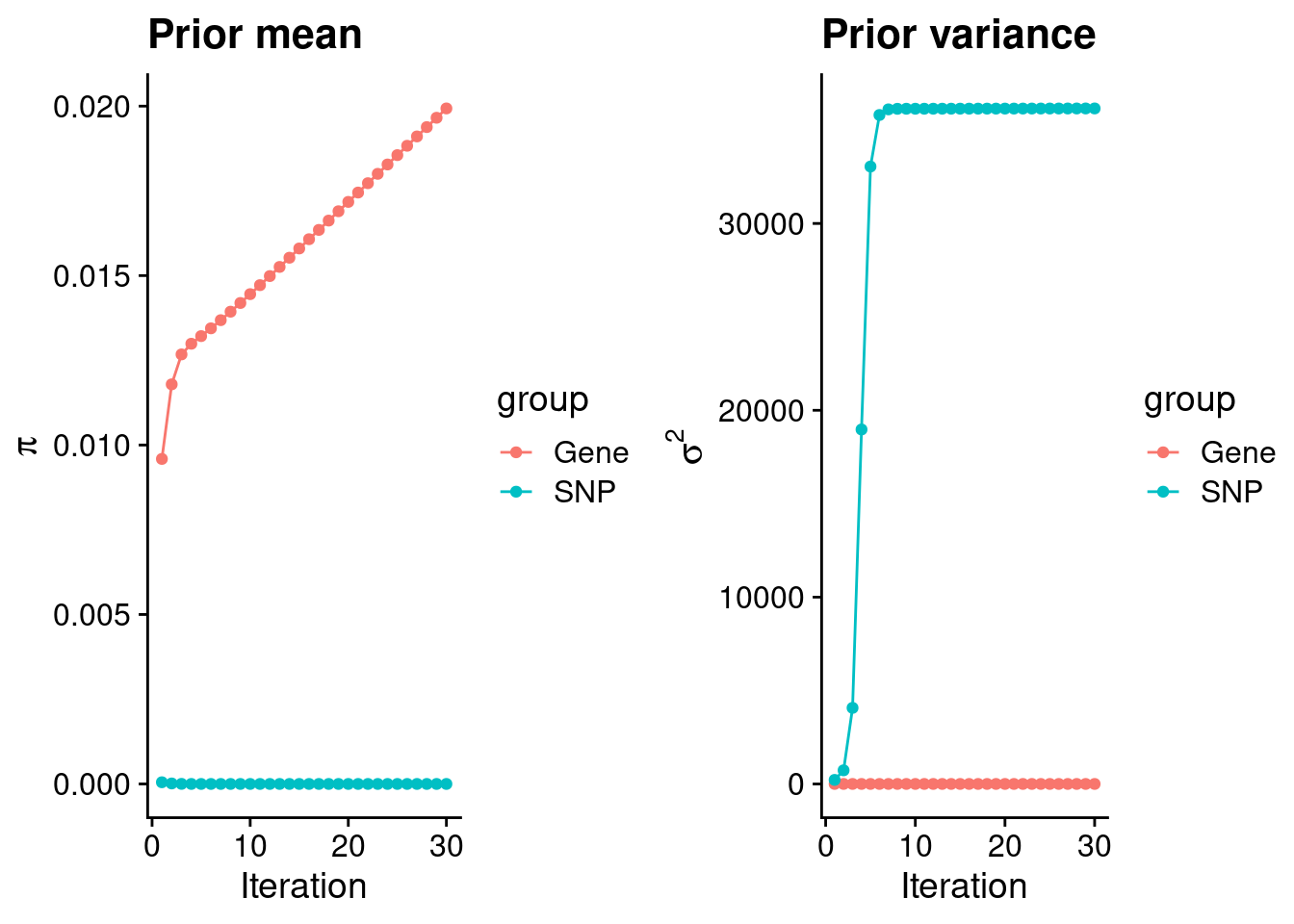

Version	Author	Date
dfd2b5f	wesleycrouse	2021-09-07

#estimated group prior
estimated_group_prior <- group_prior_rec[,ncol(group_prior_rec)]
names(estimated_group_prior) <- c("gene", "snp")
estimated_group_prior["snp"] <- estimated_group_prior["snp"]*thin #adjust parameter to account for thin argument
print(estimated_group_prior)

        gene          snp 
1.993189e-02 2.995612e-07

#estimated group prior variance
estimated_group_prior_var <- group_prior_var_rec[,ncol(group_prior_var_rec)]
names(estimated_group_prior_var) <- c("gene", "snp")
print(estimated_group_prior_var)

        gene          snp 
    1.624517 36154.672592

#report sample size
print(sample_size)

[1] 273896

#report group size
group_size <- c(nrow(ctwas_gene_res), n_snps)
print(group_size)

[1]   10901 8697330

#estimated group PVE
estimated_group_pve <- estimated_group_prior_var*estimated_group_prior*group_size/sample_size #check PVE calculation
names(estimated_group_pve) <- c("gene", "snp")
print(estimated_group_pve)

       gene         snp 
0.001288705 0.343914326

#compare sum(PIP*mu2/sample_size) with above PVE calculation
c(sum(ctwas_gene_res$PVE),sum(ctwas_snp_res$PVE))

[1] 0.0200531 0.4610330

Genes with highest PIPs

#distribution of PIPs
hist(ctwas_gene_res$susie_pip, xlim=c(0,1), main="Distribution of Gene PIPs")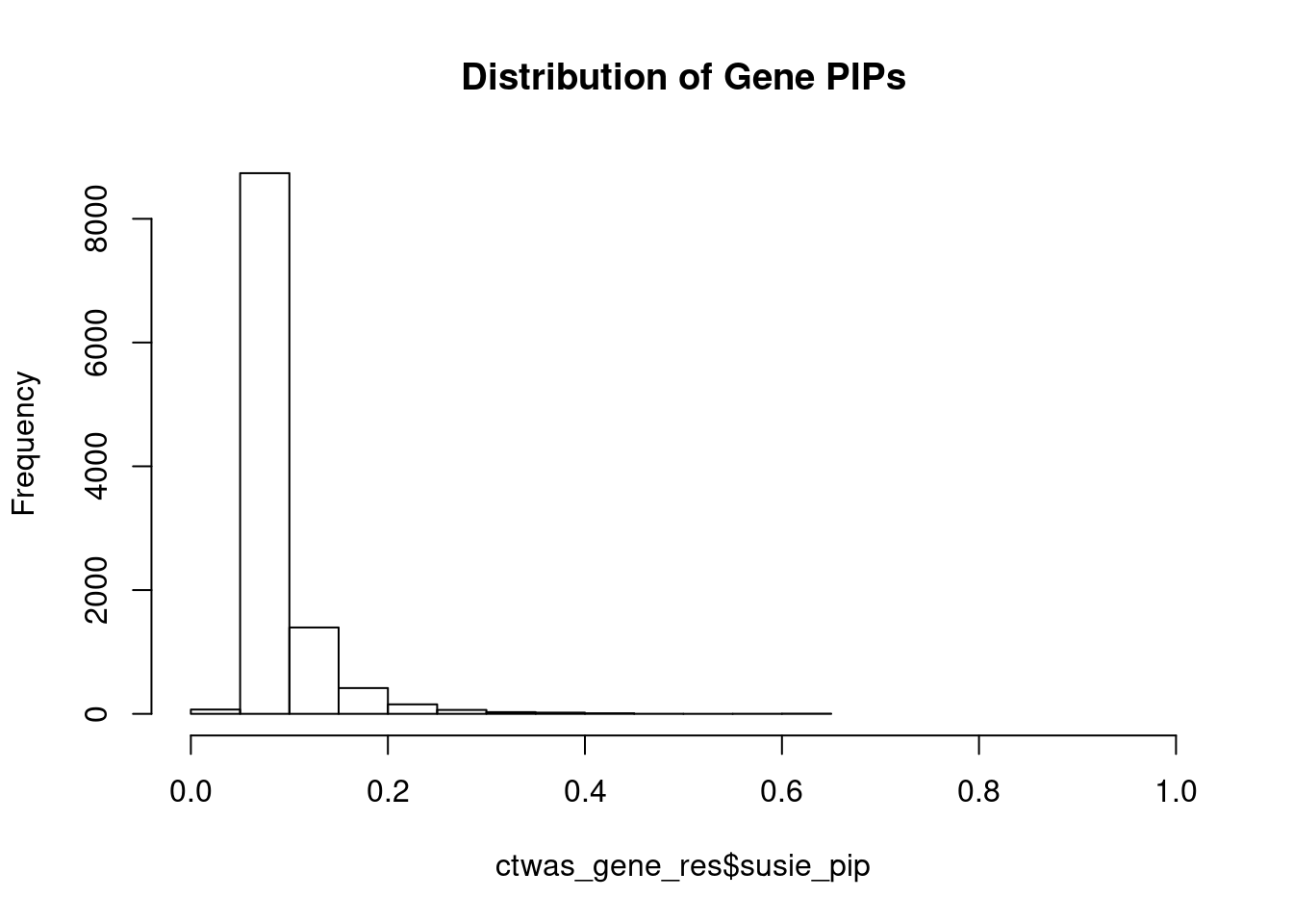

Version	Author	Date
dfd2b5f	wesleycrouse	2021-09-07

#genes with PIP>0.8 or 20 highest PIPs
head(ctwas_gene_res[order(-ctwas_gene_res$susie_pip),report_cols], max(sum(ctwas_gene_res$susie_pip>0.8), 20))

       genename region_tag susie_pip   mu2     PVE     z
7656   CATSPER2      15_16     0.629 20.97 4.8e-05 -4.75
4286      PRMT7      16_36     0.619 19.88 4.5e-05  4.56
12008       HPR      16_38     0.606 20.12 4.5e-05 -4.26
8865       FUT2      19_33     0.582 18.95 4.0e-05 -4.13
10585   HSD17B8       6_27     0.484 18.24 3.2e-05  3.74
4435      PSRC1       1_67     0.450 18.16 3.0e-05 -4.01
5648     ABHD10       3_70     0.450 16.77 2.8e-05 -3.42
6118       TEX9      15_24     0.449 17.04 2.8e-05 -3.45
8882       RHOG       11_3     0.435 17.11 2.7e-05 -3.43
5732    COMMD10       5_69     0.422 16.69 2.6e-05  3.35
12032  U91319.1      16_14     0.417 16.66 2.5e-05  3.34
8629     PHLDA3      1_101     0.413 16.39 2.5e-05 -3.30
4859     RNF121      11_40     0.405 16.00 2.4e-05  3.23
9463    EMILIN3      20_25     0.404 16.83 2.5e-05  3.45
6168     GEMIN6       2_24     0.403 16.30 2.4e-05 -3.27
9127      TSHZ1      18_44     0.400 16.26 2.4e-05 -3.26
2888      ITGB6       2_96     0.396 16.09 2.3e-05 -3.23
3272     EIF2B2      14_34     0.393 15.67 2.2e-05 -3.24
6724  TNFRSF13C      22_17     0.392 15.63 2.2e-05  3.12
463        HHAT      1_106     0.379 15.83 2.2e-05  3.17

Genes with largest effect sizes

#plot PIP vs effect size
plot(ctwas_gene_res$susie_pip, ctwas_gene_res$mu2, xlab="PIP", ylab="mu^2", main="Gene PIPs vs Effect Size")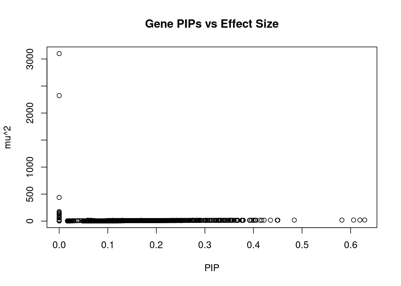

Version	Author	Date
dfd2b5f	wesleycrouse	2021-09-07

#genes with 20 largest effect sizes
head(ctwas_gene_res[order(-ctwas_gene_res$mu2),report_cols],20)

          genename region_tag susie_pip     mu2     PVE      z
10435          LPA      6_104     0.000 3100.25 0.0e+00  60.08
5799       SLC22A3      6_104     0.000 2321.99 0.0e+00 -80.70
3449           PLG      6_104     0.000  437.35 0.0e+00  48.04
5796          WTAP      6_103     0.000  175.68 0.0e+00   7.02
11043   RP1-81D8.3      6_104     0.000  165.64 0.0e+00 -62.47
1074        MAP3K4      6_104     0.000  148.80 0.0e+00  24.06
11375 RP3-393E18.2      6_103     0.000  135.84 0.0e+00 -13.28
2628          SOD2      6_103     0.000  118.12 0.0e+00  -7.20
2629        MRPL18      6_103     0.000  109.26 0.0e+00  -6.69
5795        PNLDC1      6_103     0.000   79.01 0.0e+00   4.09
5793        DYNLT1      6_103     0.000   66.15 0.0e+00  -6.33
7349         SYTL3      6_103     0.000   58.48 0.0e+00   5.73
4070         RSPH3      6_103     0.000   26.92 0.0e+00   3.37
7656      CATSPER2      15_16     0.629   20.97 4.8e-05  -4.75
10185        IGF2R      6_103     0.000   20.68 0.0e+00  -8.46
12008          HPR      16_38     0.606   20.12 4.5e-05  -4.26
4286         PRMT7      16_36     0.619   19.88 4.5e-05   4.56
8865          FUT2      19_33     0.582   18.95 4.0e-05  -4.13
10585      HSD17B8       6_27     0.484   18.24 3.2e-05   3.74
4435         PSRC1       1_67     0.450   18.16 3.0e-05  -4.01

Genes with highest PVE

#genes with 20 highest pve
head(ctwas_gene_res[order(-ctwas_gene_res$PVE),report_cols],20)

      genename region_tag susie_pip   mu2     PVE     z
7656  CATSPER2      15_16     0.629 20.97 4.8e-05 -4.75
4286     PRMT7      16_36     0.619 19.88 4.5e-05  4.56
12008      HPR      16_38     0.606 20.12 4.5e-05 -4.26
8865      FUT2      19_33     0.582 18.95 4.0e-05 -4.13
10585  HSD17B8       6_27     0.484 18.24 3.2e-05  3.74
4435     PSRC1       1_67     0.450 18.16 3.0e-05 -4.01
5648    ABHD10       3_70     0.450 16.77 2.8e-05 -3.42
6118      TEX9      15_24     0.449 17.04 2.8e-05 -3.45
8882      RHOG       11_3     0.435 17.11 2.7e-05 -3.43
5732   COMMD10       5_69     0.422 16.69 2.6e-05  3.35
8629    PHLDA3      1_101     0.413 16.39 2.5e-05 -3.30
12032 U91319.1      16_14     0.417 16.66 2.5e-05  3.34
9463   EMILIN3      20_25     0.404 16.83 2.5e-05  3.45
6168    GEMIN6       2_24     0.403 16.30 2.4e-05 -3.27
4859    RNF121      11_40     0.405 16.00 2.4e-05  3.23
9127     TSHZ1      18_44     0.400 16.26 2.4e-05 -3.26
2888     ITGB6       2_96     0.396 16.09 2.3e-05 -3.23
463       HHAT      1_106     0.379 15.83 2.2e-05  3.17
4653  SERPINE2      2_132     0.378 15.86 2.2e-05 -3.16
2240   SEC23IP      10_74     0.377 16.00 2.2e-05  3.70

Genes with largest z scores

#genes with 20 largest z scores
head(ctwas_gene_res[order(-abs(ctwas_gene_res$z)),report_cols],20)

          genename region_tag susie_pip     mu2     PVE      z
5799       SLC22A3      6_104     0.000 2321.99 0.0e+00 -80.70
11043   RP1-81D8.3      6_104     0.000  165.64 0.0e+00 -62.47
10435          LPA      6_104     0.000 3100.25 0.0e+00  60.08
3449           PLG      6_104     0.000  437.35 0.0e+00  48.04
1074        MAP3K4      6_104     0.000  148.80 0.0e+00  24.06
11375 RP3-393E18.2      6_103     0.000  135.84 0.0e+00 -13.28
10185        IGF2R      6_103     0.000   20.68 0.0e+00  -8.46
2628          SOD2      6_103     0.000  118.12 0.0e+00  -7.20
5796          WTAP      6_103     0.000  175.68 0.0e+00   7.02
2629        MRPL18      6_103     0.000  109.26 0.0e+00  -6.69
5793        DYNLT1      6_103     0.000   66.15 0.0e+00  -6.33
5240         NLRC5      16_31     0.059   17.83 3.8e-06   6.20
7349         SYTL3      6_103     0.000   58.48 0.0e+00   5.73
1120          CETP      16_31     0.065   16.09 3.8e-06   5.71
7656      CATSPER2      15_16     0.629   20.97 4.8e-05  -4.75
4286         PRMT7      16_36     0.619   19.88 4.5e-05   4.56
12008          HPR      16_38     0.606   20.12 4.5e-05  -4.26
8865          FUT2      19_33     0.582   18.95 4.0e-05  -4.13
5795        PNLDC1      6_103     0.000   79.01 0.0e+00   4.09
4435         PSRC1       1_67     0.450   18.16 3.0e-05  -4.01

Comparing z scores and PIPs

#set nominal signifiance threshold for z scores
alpha <- 0.05

#bonferroni adjusted threshold for z scores
sig_thresh <- qnorm(1-(alpha/nrow(ctwas_gene_res)/2), lower=T)

#Q-Q plot for z scores
obs_z <- ctwas_gene_res$z[order(ctwas_gene_res$z)]
exp_z <- qnorm((1:nrow(ctwas_gene_res))/nrow(ctwas_gene_res))

plot(exp_z, obs_z, xlab="Expected z", ylab="Observed z", main="Gene z score Q-Q plot")
abline(a=0,b=1)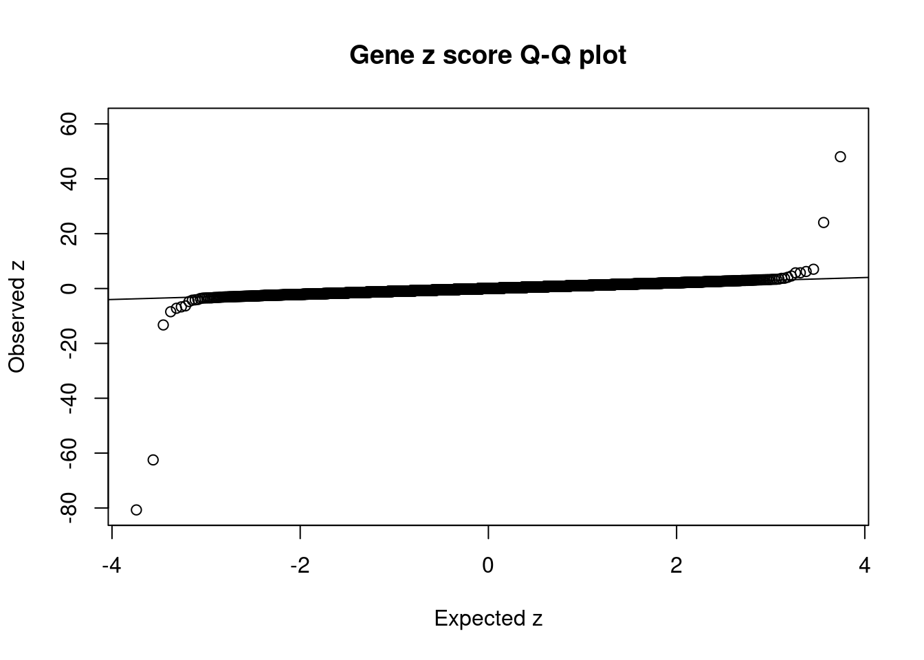

Version	Author	Date
dfd2b5f	wesleycrouse	2021-09-07

#plot z score vs PIP
plot(abs(ctwas_gene_res$z), ctwas_gene_res$susie_pip, xlab="abs(z)", ylab="PIP")
abline(v=sig_thresh, col="red", lty=2)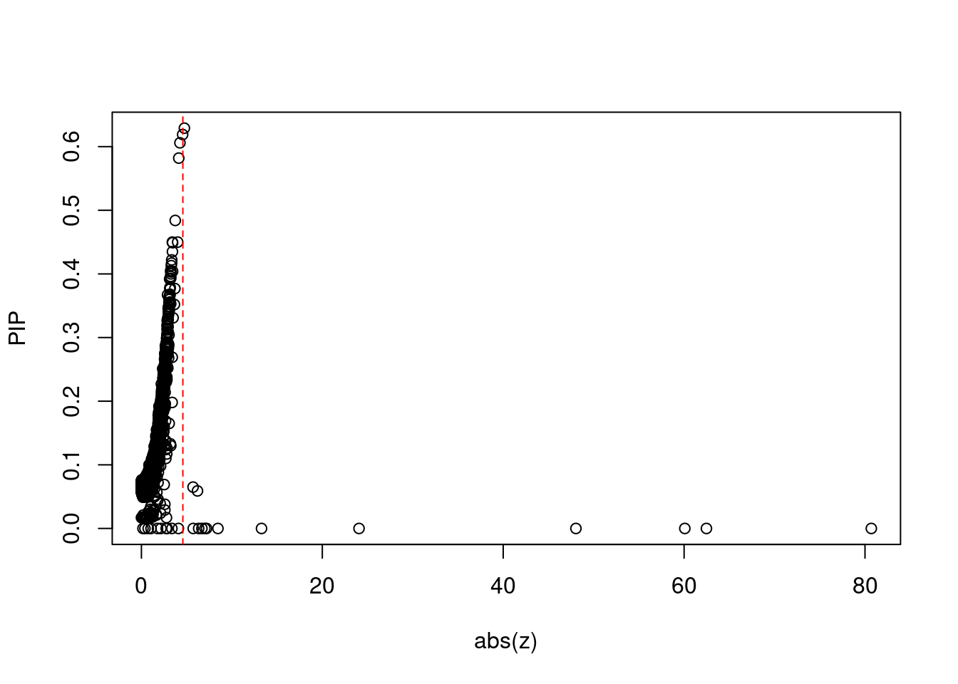

Version	Author	Date
dfd2b5f	wesleycrouse	2021-09-07

#proportion of significant z scores
mean(abs(ctwas_gene_res$z) > sig_thresh)

[1] 0.001376021

#genes with most significant z scores
head(ctwas_gene_res[order(-abs(ctwas_gene_res$z)),report_cols],20)

          genename region_tag susie_pip     mu2     PVE      z
5799       SLC22A3      6_104     0.000 2321.99 0.0e+00 -80.70
11043   RP1-81D8.3      6_104     0.000  165.64 0.0e+00 -62.47
10435          LPA      6_104     0.000 3100.25 0.0e+00  60.08
3449           PLG      6_104     0.000  437.35 0.0e+00  48.04
1074        MAP3K4      6_104     0.000  148.80 0.0e+00  24.06
11375 RP3-393E18.2      6_103     0.000  135.84 0.0e+00 -13.28
10185        IGF2R      6_103     0.000   20.68 0.0e+00  -8.46
2628          SOD2      6_103     0.000  118.12 0.0e+00  -7.20
5796          WTAP      6_103     0.000  175.68 0.0e+00   7.02
2629        MRPL18      6_103     0.000  109.26 0.0e+00  -6.69
5793        DYNLT1      6_103     0.000   66.15 0.0e+00  -6.33
5240         NLRC5      16_31     0.059   17.83 3.8e-06   6.20
7349         SYTL3      6_103     0.000   58.48 0.0e+00   5.73
1120          CETP      16_31     0.065   16.09 3.8e-06   5.71
7656      CATSPER2      15_16     0.629   20.97 4.8e-05  -4.75
4286         PRMT7      16_36     0.619   19.88 4.5e-05   4.56
12008          HPR      16_38     0.606   20.12 4.5e-05  -4.26
8865          FUT2      19_33     0.582   18.95 4.0e-05  -4.13
5795        PNLDC1      6_103     0.000   79.01 0.0e+00   4.09
4435         PSRC1       1_67     0.450   18.16 3.0e-05  -4.01

Locus plots for genes and SNPs

ctwas_gene_res_sortz <- ctwas_gene_res[order(-abs(ctwas_gene_res$z)),]

n_plots <- 5
for (region_tag_plot in head(unique(ctwas_gene_res_sortz$region_tag), n_plots)){
  ctwas_res_region <-  ctwas_res[ctwas_res$region_tag==region_tag_plot,]
  start <- min(ctwas_res_region$pos)
  end <- max(ctwas_res_region$pos)
  
  ctwas_res_region <- ctwas_res_region[order(ctwas_res_region$pos),]
  ctwas_res_region_gene <- ctwas_res_region[ctwas_res_region$type=="gene",]
  ctwas_res_region_snp <- ctwas_res_region[ctwas_res_region$type=="SNP",]
  
  #region name
  print(paste0("Region: ", region_tag_plot))
  
  #table of genes in region
  print(ctwas_res_region_gene[,report_cols])
  
  par(mfrow=c(4,1))
  
  #gene z scores
  plot(ctwas_res_region_gene$pos, abs(ctwas_res_region_gene$z), xlab="Position", ylab="abs(gene_z)", xlim=c(start,end),
   ylim=c(0,max(sig_thresh, abs(ctwas_res_region_gene$z))),
   main=paste0("Region: ", region_tag_plot))
  abline(h=sig_thresh,col="red",lty=2)
  
  #significance threshold for SNPs
  alpha_snp <- 5*10^(-8)
  sig_thresh_snp <- qnorm(1-alpha_snp/2, lower=T)
  
  #snp z scores
  plot(ctwas_res_region_snp$pos, abs(ctwas_res_region_snp$z), xlab="Position", ylab="abs(snp_z)",xlim=c(start,end),
   ylim=c(0,max(sig_thresh_snp, max(abs(ctwas_res_region_snp$z)))))
  abline(h=sig_thresh_snp,col="purple",lty=2)
  
  #gene pips
  plot(ctwas_res_region_gene$pos, ctwas_res_region_gene$susie_pip, xlab="Position", ylab="Gene PIP", xlim=c(start,end), ylim=c(0,1))
  abline(h=0.8,col="blue",lty=2)
  
  #snp pips
  plot(ctwas_res_region_snp$pos, ctwas_res_region_snp$susie_pip, xlab="Position", ylab="SNP PIP", xlim=c(start,end), ylim=c(0,1))
  abline(h=0.8,col="blue",lty=2)
}

[1] "Region: 6_104"
        genename region_tag susie_pip     mu2 PVE      z
5799     SLC22A3      6_104         0 2321.99   0 -80.70
10435        LPA      6_104         0 3100.25   0  60.08
11043 RP1-81D8.3      6_104         0  165.64   0 -62.47
3449         PLG      6_104         0  437.35   0  48.04
1074      MAP3K4      6_104         0  148.80   0  24.06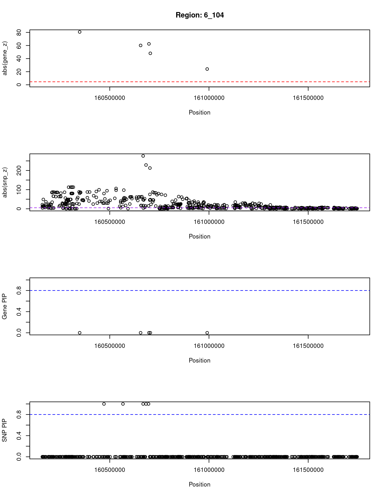

Version	Author	Date
dfd2b5f	wesleycrouse	2021-09-07

[1] "Region: 6_103"
          genename region_tag susie_pip    mu2 PVE      z
911          SYNJ2      6_103         0   3.52   0   0.39
3456        SERAC1      6_103         0  17.11   0   2.74
12288       GTF2H5      6_103         0   6.42   0  -1.06
4067         TULP4      6_103         0   4.94   0   0.75
5793        DYNLT1      6_103         0  66.15   0  -6.33
7349         SYTL3      6_103         0  58.48   0   5.73
1290           EZR      6_103         0   8.33   0  -1.78
10532      C6orf99      6_103         0   3.29   0  -0.17
4070         RSPH3      6_103         0  26.92   0   3.37
7351         TAGAP      6_103         0  15.98   0   2.85
11375 RP3-393E18.2      6_103         0 135.84   0 -13.28
5796          WTAP      6_103         0 175.68   0   7.02
2628          SOD2      6_103         0 118.12   0  -7.20
3332          TCP1      6_103         0  16.71   0  -2.16
2629        MRPL18      6_103         0 109.26   0  -6.69
5795        PNLDC1      6_103         0  79.01   0   4.09
10185        IGF2R      6_103         0  20.68   0  -8.46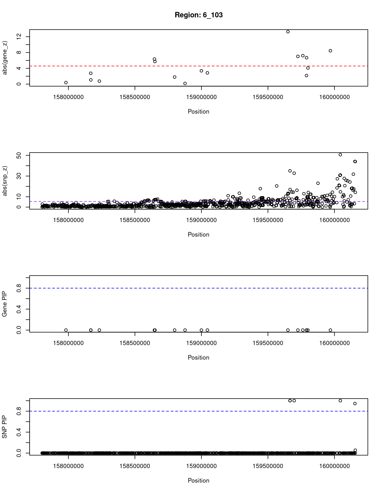

Version	Author	Date
dfd2b5f	wesleycrouse	2021-09-07

[1] "Region: 16_31"
          genename region_tag susie_pip   mu2     PVE     z
6688         CES5A      16_31     0.086  5.29 1.7e-06  0.83
1124         GNAO1      16_31     0.060  3.24 7.1e-07  0.32
11561 RP11-461O7.1      16_31     0.078  4.73 1.3e-06  0.77
6695          AMFR      16_31     0.059  3.27 7.1e-07  0.65
7710        NUDT21      16_31     0.067  3.88 9.5e-07  0.61
3681          BBS2      16_31     0.062  3.51 7.9e-07  0.70
1122           MT3      16_31     0.060  3.22 7.1e-07  0.04
8094          MT1E      16_31     0.170  9.80 6.1e-06 -2.03
10727         MT1M      16_31     0.064  4.12 9.6e-07  1.29
10725         MT1A      16_31     0.110  7.56 3.0e-06  1.99
10386         MT1F      16_31     0.061  3.50 7.8e-07  0.84
9805          MT1X      16_31     0.066  3.75 9.1e-07  0.39
1740         NUP93      16_31     0.069  4.13 1.0e-06 -0.73
438        HERPUD1      16_31     0.065  4.12 9.7e-07  1.13
1120          CETP      16_31     0.065 16.09 3.8e-06  5.71
5240         NLRC5      16_31     0.059 17.83 3.8e-06  6.20
5239         CPNE2      16_31     0.064  3.61 8.4e-07  0.50
8472       FAM192A      16_31     0.072  4.48 1.2e-06 -1.03
6698        RSPRY1      16_31     0.100  6.02 2.2e-06  0.84
1745          PLLP      16_31     0.060  3.34 7.3e-07 -0.62
81          CX3CL1      16_31     0.064  3.73 8.7e-07 -0.84
1747         CCL17      16_31     0.082  5.36 1.6e-06 -1.29
52         CIAPIN1      16_31     0.065  3.87 9.2e-07 -0.83
1154          COQ9      16_31     0.078  4.90 1.4e-06 -1.01
3685          DOK4      16_31     0.059  3.13 6.8e-07  0.00
4628      CCDC102A      16_31     0.118  7.64 3.3e-06  1.69
10722       ADGRG1      16_31     0.059  3.10 6.6e-07  0.04
9366        ADGRG3      16_31     0.080  5.04 1.5e-06  1.05
5241        KATNB1      16_31     0.060  3.23 7.1e-07 -0.28
5242         KIFC3      16_31     0.068  3.98 9.8e-07  0.69
1754          USB1      16_31     0.065  3.77 9.0e-07  0.61
7571        ZNF319      16_31     0.061  3.35 7.5e-07  0.38
1753         MMP15      16_31     0.063  3.53 8.1e-07  0.47
729         CFAP20      16_31     0.081  5.14 1.5e-06  1.08
730        CSNK2A2      16_31     0.059  3.11 6.7e-07  0.10
9278         GINS3      16_31     0.073  4.46 1.2e-06  0.88
1757         NDRG4      16_31     0.064  3.66 8.6e-07 -0.56
3680         CNOT1      16_31     0.072  4.35 1.1e-06  0.85
1759       SLC38A7      16_31     0.081  5.13 1.5e-06  1.09
3684          GOT2      16_31     0.086  5.54 1.7e-06 -1.19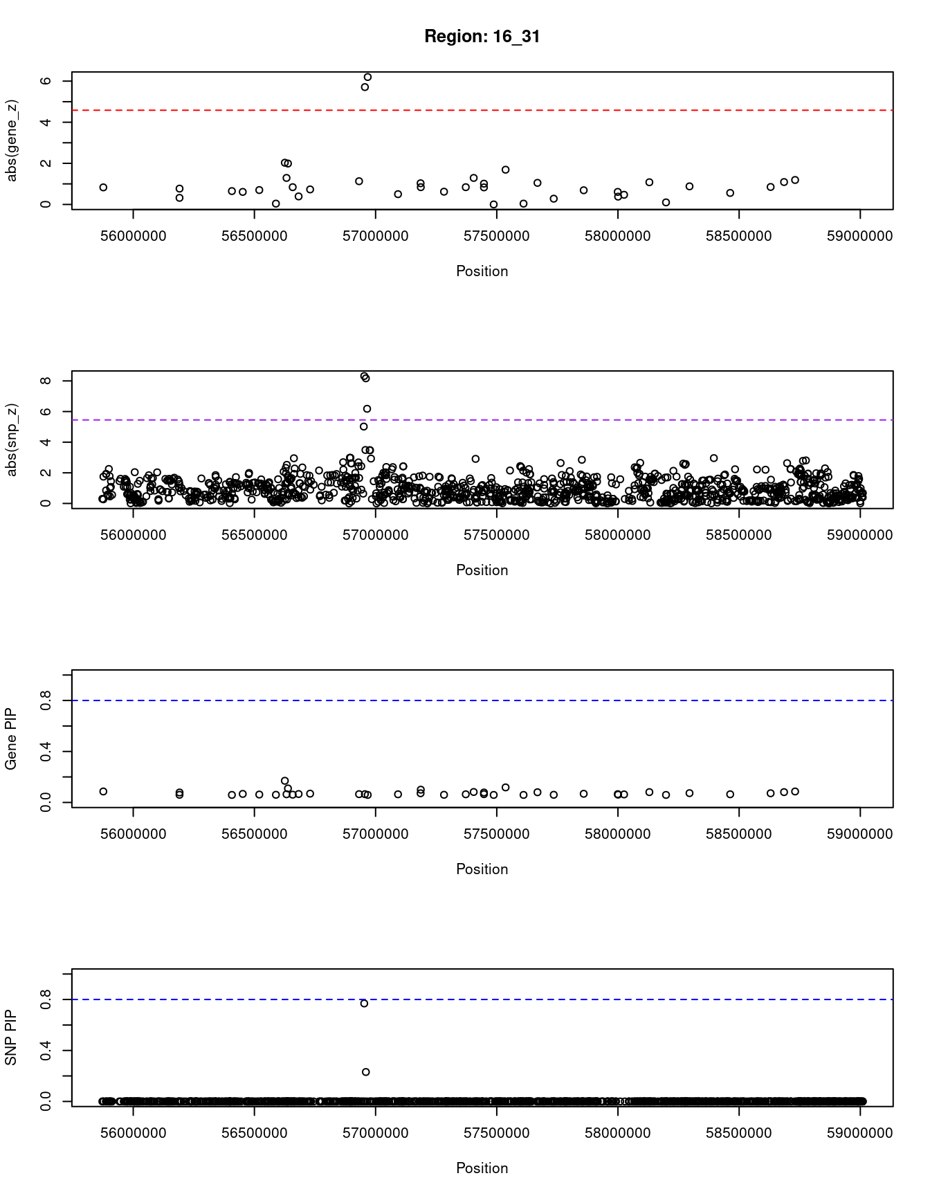

Version	Author	Date
dfd2b5f	wesleycrouse	2021-09-07

[1] "Region: 15_16"
     genename region_tag susie_pip   mu2     PVE     z
1853   ZNF106      15_16     0.055  3.79 7.6e-07  1.00
9202   LRRC57      15_16     0.053  3.55 6.9e-07  0.63
6691   STARD9      15_16     0.054  3.69 7.3e-07 -0.66
5189    CDAN1      15_16     0.056  3.97 8.2e-07  0.66
3962    TTBK2      15_16     0.131  9.38 4.5e-06 -1.99
4903   TMEM62      15_16     0.056  3.89 7.9e-07 -0.83
7984     ADAL      15_16     0.052  3.48 6.6e-07  1.41
7985    LCMT2      15_16     0.133  9.49 4.6e-06  3.20
4898  TUBGCP4      15_16     0.057  4.03 8.4e-07 -1.71
5180  ZSCAN29      15_16     0.053  3.57 6.9e-07 -0.13
7702    MAP1A      15_16     0.198 12.12 8.7e-06 -3.40
7656 CATSPER2      15_16     0.629 20.97 4.8e-05 -4.75
7709    PDIA3      15_16     0.050  3.26 6.0e-07 -0.21
5178    MFAP1      15_16     0.117  8.64 3.7e-06 -2.80
1286    WDR76      15_16     0.126  9.11 4.2e-06 -2.83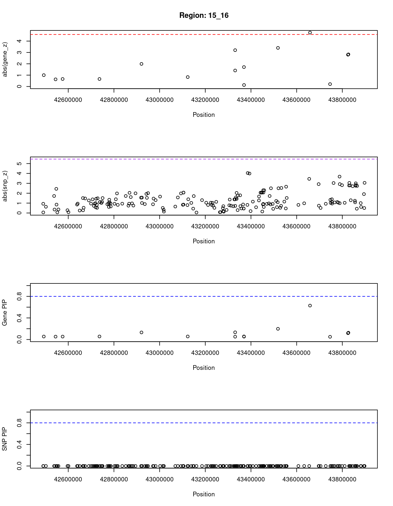

Version	Author	Date
dfd2b5f	wesleycrouse	2021-09-07

[1] "Region: 16_36"
       genename region_tag susie_pip   mu2     PVE     z
11566 LINC00920      16_36     0.110  7.32 2.9e-06  1.42
7635      BEAN1      16_36     0.064  3.83 8.9e-07  0.51
7636        TK2      16_36     0.085  5.69 1.8e-06 -1.21
10968      CKLF      16_36     0.085  5.69 1.8e-06  1.21
1195      CMTM1      16_36     0.057  3.12 6.5e-07  0.04
5245      CMTM3      16_36     0.067  4.11 1.0e-06 -0.55
9452      CMTM4      16_36     0.109  7.27 2.9e-06  1.84
4626   DYNC1LI2      16_36     0.065  3.94 9.3e-07 -1.11
6700       NAE1      16_36     0.058  3.19 6.7e-07 -0.36
7643     FAM96B      16_36     0.060  3.47 7.7e-07 -0.30
8480       CES3      16_36     0.057  3.11 6.5e-07 -0.47
661        CBFB      16_36     0.060  3.40 7.4e-07 -0.73
3683   C16orf70      16_36     0.070  4.43 1.1e-06  0.63
10022 KIAA0895L      16_36     0.086  5.73 1.8e-06 -1.40
9065    EXOC3L1      16_36     0.057  3.11 6.5e-07  0.30
10715      E2F4      16_36     0.057  3.12 6.5e-07 -0.24
1737      ELMO3      16_36     0.151  9.38 5.2e-06  2.45
4629     SLC9A5      16_36     0.060  3.42 7.5e-07  0.77
4627      FHOD1      16_36     0.064  3.81 8.8e-07  0.88
6708      TPPP3      16_36     0.078  5.11 1.5e-06 -1.50
1748       CTCF      16_36     0.061  3.56 7.9e-07 -0.41
1749        ACD      16_36     0.058  3.19 6.7e-07 -0.15
1751     PARD6A      16_36     0.058  3.19 6.7e-07 -0.15
3584      ENKD1      16_36     0.057  3.13 6.5e-07 -0.06
5272      GFOD2      16_36     0.061  3.53 7.8e-07 -0.46
1741   TSNAXIP1      16_36     0.061  3.51 7.8e-07  1.08
5271    RANBP10      16_36     0.057  3.10 6.5e-07 -0.02
1739      NUTF2      16_36     0.057  3.10 6.4e-07 -0.04
6713      PSKH1      16_36     0.138  8.81 4.4e-06 -2.69
10714    PSMB10      16_36     0.057  3.10 6.4e-07 -0.13
9360      DDX28      16_36     0.165  9.98 6.0e-06  3.07
770      NFATC3      16_36     0.124  8.08 3.6e-06 -2.71
1765      ESRP2      16_36     0.098  6.60 2.4e-06  2.12
1764    PLA2G15      16_36     0.059  3.30 7.1e-07 -0.74
1763     SLC7A6      16_36     0.080  5.26 1.5e-06 -1.39
4286      PRMT7      16_36     0.619 19.88 4.5e-05  4.56
9563      ZFP90      16_36     0.096  6.47 2.3e-06  1.33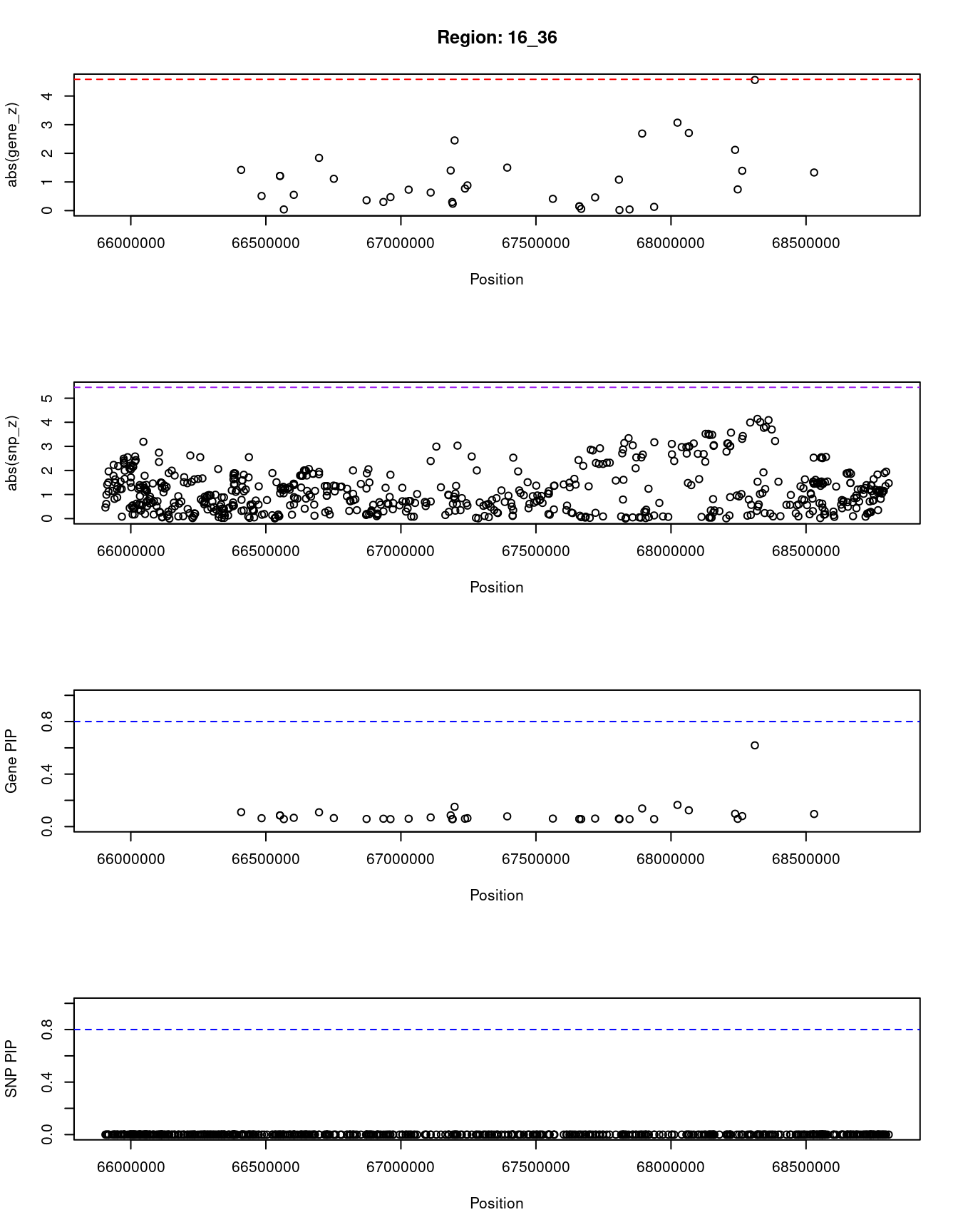

Version	Author	Date
dfd2b5f	wesleycrouse	2021-09-07

SNPs with highest PIPs

#snps with PIP>0.8 or 20 highest PIPs
head(ctwas_snp_res[order(-ctwas_snp_res$susie_pip),report_cols_snps],
max(sum(ctwas_snp_res$susie_pip>0.8), 20))

                id region_tag susie_pip      mu2     PVE      z
376634 rs185885155      6_103     1.000  1298.05 4.7e-03  35.03
376636   rs2842983      6_103     1.000   461.56 1.7e-03  17.01
376644 rs117055069      6_103     1.000   624.86 2.3e-03  32.73
376751    rs688359      6_103     1.000  1814.23 6.6e-03 -50.66
376910 rs182443492      6_104     1.000  6801.55 2.5e-02  79.64
376928 rs141383002      6_104     1.000  8049.15 2.9e-02 -12.40
376955  rs56393506      6_104     1.000 67286.67 2.5e-01 275.91
376962 rs374071816      6_104     1.000 29248.69 1.1e-01 228.59
376963   rs9458002      6_104     1.000  6913.57 2.5e-02  15.22
821102 rs113345881      19_32     1.000    85.02 3.1e-04  -9.42
821105  rs12721109      19_32     1.000    67.73 2.5e-04  -7.62
775778   rs1801689      17_38     0.977    48.96 1.7e-04   6.65
376784   rs1443844      6_103     0.945  1461.62 5.0e-03 -44.12
821067 rs111794050      19_32     0.883    50.33 1.6e-04  -7.44
745890  rs12446515      16_31     0.769    73.96 2.1e-04  -8.32
821095  rs34878901      19_32     0.360    96.37 1.3e-04   7.49
745892    rs821840      16_31     0.231    71.57 6.0e-05  -8.17
821092   rs8106922      19_32     0.084    86.21 2.7e-05   7.20
376785   rs3818678      6_103     0.055  1462.14 3.0e-04 -44.02
377558  rs76667746      6_105     0.055   139.97 2.8e-05   5.50

SNPs with largest effect sizes

#plot PIP vs effect size
plot(ctwas_snp_res$susie_pip, ctwas_snp_res$mu2, xlab="PIP", ylab="mu^2", main="SNP PIPs vs Effect Size")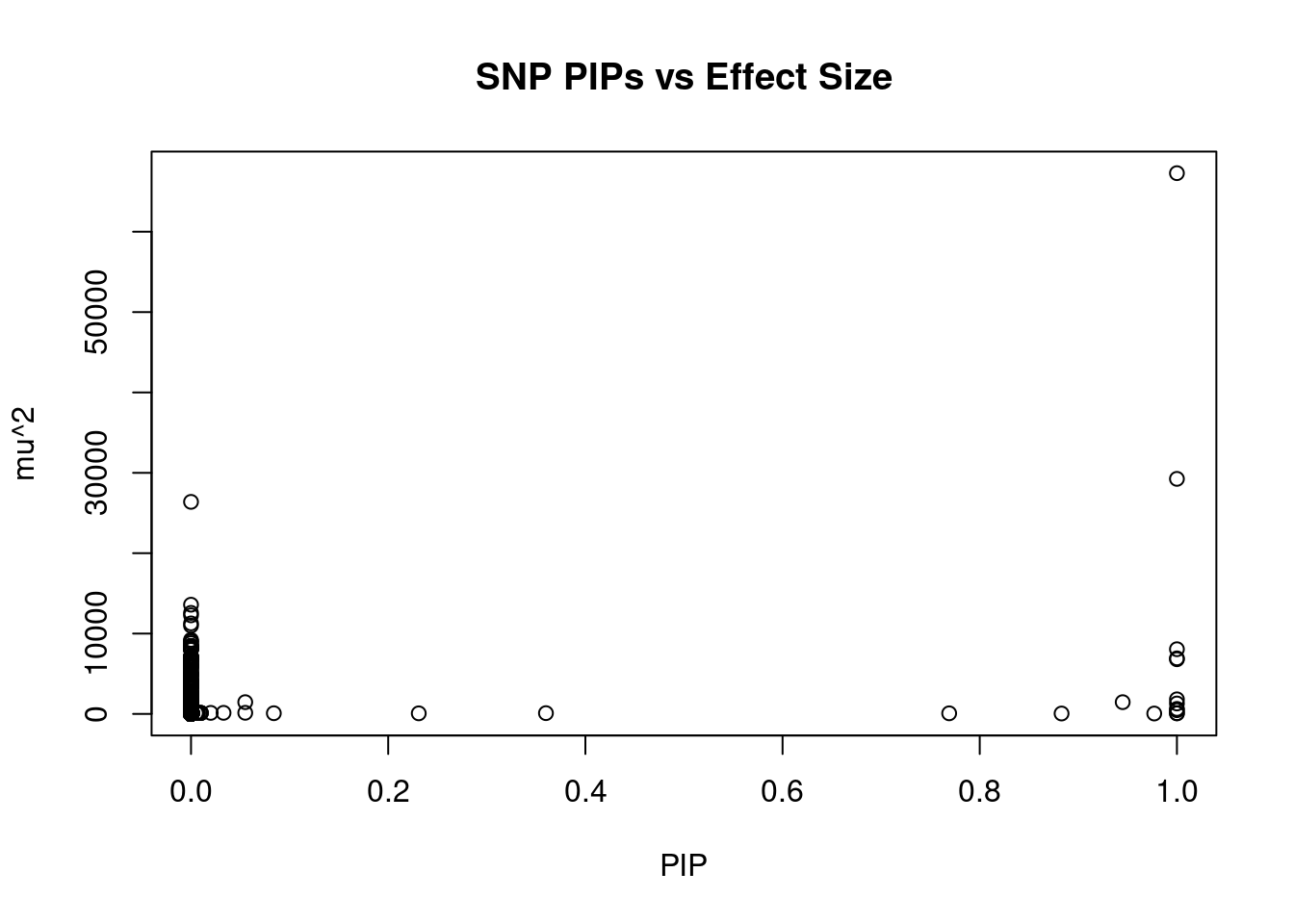

Version	Author	Date
dfd2b5f	wesleycrouse	2021-09-07

#SNPs with 50 largest effect sizes
head(ctwas_snp_res[order(-ctwas_snp_res$mu2),report_cols_snps],50)

                id region_tag susie_pip      mu2     PVE      z
376955  rs56393506      6_104         1 67286.67 2.5e-01 275.91
376962 rs374071816      6_104         1 29248.69 1.1e-01 228.59
376967   rs4252185      6_104         0 26385.89 0.0e+00 212.79
376921   rs3124784      6_104         0 13588.94 0.0e+00 106.12
376922   rs3127596      6_104         0 12573.24 0.0e+00  96.83
376915   rs3127599      6_104         0 12266.73 0.0e+00  94.24
376953   rs9365200      6_104         0 11262.91 0.0e+00  63.20
376919 rs117733303      6_104         0 10983.45 0.0e+00  44.24
376899   rs1510226      6_104         0  9214.94 0.0e+00  40.59
376971    rs783147      6_104         0  9034.42 0.0e+00 -87.24
376906   rs9355288      6_104         0  9012.73 0.0e+00  99.30
376966   rs2314851      6_104         0  8795.09 0.0e+00  75.18
376879   rs3106167      6_104         0  8450.88 0.0e+00 112.93
376870   rs3106169      6_104         0  8450.04 0.0e+00 112.93
376871   rs3127598      6_104         0  8447.02 0.0e+00 112.91
376863  rs11755965      6_104         0  8443.74 0.0e+00 112.90
376854  rs12194962      6_104         0  8422.52 0.0e+00 112.68
376872   rs3127597      6_104         0  8374.08 0.0e+00 112.65
376943   rs9355814      6_104         0  8250.71 0.0e+00 -62.25
376948  rs36115561      6_104         0  8246.29 0.0e+00 -62.12
376950   rs2092931      6_104         0  8225.50 0.0e+00  61.87
376940   rs6455692      6_104         0  8224.87 0.0e+00 -61.80
376941   rs7769720      6_104         0  8219.46 0.0e+00 -61.75
376942   rs6932014      6_104         0  8218.89 0.0e+00 -61.75
376949  rs10945683      6_104         0  8210.24 0.0e+00 -61.76
376974   rs9458016      6_104         0  8079.69 0.0e+00 -83.48
376928 rs141383002      6_104         1  8049.15 2.9e-02 -12.40
376945   rs7765684      6_104         0  8045.24 0.0e+00 -60.80
376975   rs4252125      6_104         0  8035.29 0.0e+00 -83.37
376959   rs1590183      6_104         0  7973.39 0.0e+00  52.93
376978  rs80276688      6_104         0  7153.35 0.0e+00 -79.28
376936 rs117945468      6_104         0  7145.95 0.0e+00  17.54
376946   rs7746273      6_104         0  7141.24 0.0e+00 -53.48
376970     rs14224      6_104         0  7095.04 0.0e+00  36.31
376956 rs117830977      6_104         0  7039.47 0.0e+00  16.81
376900   rs2872317      6_104         0  6988.96 0.0e+00  87.72
376891    rs624319      6_104         0  6984.47 0.0e+00 -86.58
376897   rs2313453      6_104         0  6981.38 0.0e+00  87.68
376963   rs9458002      6_104         1  6913.57 2.5e-02  15.22
376910 rs182443492      6_104         1  6801.55 2.5e-02  79.64
376961  rs58247541      6_104         0  6795.61 2.3e-06  15.50
376933   rs9457943      6_104         0  6720.67 0.0e+00 -43.87
376934   rs6923877      6_104         0  6718.91 0.0e+00 -43.96
376890    rs637614      6_104         0  6714.07 0.0e+00 -85.42
376929   rs9365174      6_104         0  6683.38 0.0e+00 -44.67
376892    rs486339      6_104         0  6682.45 0.0e+00 -85.10
376965   rs1950562      6_104         0  6535.18 0.0e+00  45.64
376964   rs1864450      6_104         0  6534.46 0.0e+00  45.69
376903    rs388170      6_104         0  6413.35 0.0e+00  90.40
376987  rs60198722      6_104         0  6180.19 0.0e+00 -74.97

SNPs with highest PVE

#SNPs with 50 highest pve
head(ctwas_snp_res[order(-ctwas_snp_res$PVE),report_cols_snps],50)

                id region_tag susie_pip      mu2     PVE      z
376955  rs56393506      6_104     1.000 67286.67 2.5e-01 275.91
376962 rs374071816      6_104     1.000 29248.69 1.1e-01 228.59
376928 rs141383002      6_104     1.000  8049.15 2.9e-02 -12.40
376910 rs182443492      6_104     1.000  6801.55 2.5e-02  79.64
376963   rs9458002      6_104     1.000  6913.57 2.5e-02  15.22
376751    rs688359      6_103     1.000  1814.23 6.6e-03 -50.66
376784   rs1443844      6_103     0.945  1461.62 5.0e-03 -44.12
376634 rs185885155      6_103     1.000  1298.05 4.7e-03  35.03
376644 rs117055069      6_103     1.000   624.86 2.3e-03  32.73
376636   rs2842983      6_103     1.000   461.56 1.7e-03  17.01
821102 rs113345881      19_32     1.000    85.02 3.1e-04  -9.42
376785   rs3818678      6_103     0.055  1462.14 3.0e-04 -44.02
821105  rs12721109      19_32     1.000    67.73 2.5e-04  -7.62
745890  rs12446515      16_31     0.769    73.96 2.1e-04  -8.32
775778   rs1801689      17_38     0.977    48.96 1.7e-04   6.65
821067 rs111794050      19_32     0.883    50.33 1.6e-04  -7.44
821095  rs34878901      19_32     0.360    96.37 1.3e-04   7.49
745892    rs821840      16_31     0.231    71.57 6.0e-05  -8.17
377558  rs76667746      6_105     0.055   139.97 2.8e-05   5.50
821092   rs8106922      19_32     0.084    86.21 2.7e-05   7.20
377931  rs55902653      6_106     0.033   134.66 1.6e-05  -5.21
377560   rs2023073      6_105     0.020   129.90 9.7e-06   5.30
810578 rs147985405       19_9     0.010   121.53 4.6e-06  -5.14
810571 rs138175288       19_9     0.010   121.38 4.5e-06  -5.14
810572 rs138294113       19_9     0.010   120.96 4.3e-06  -5.13
810575 rs112552009       19_9     0.009   119.64 3.8e-06  -5.10
810573  rs73015020       19_9     0.007   117.73 3.1e-06  -5.06
810570  rs55997232       19_9     0.007   117.26 2.9e-06  -5.05
810576  rs10412048       19_9     0.006   115.37 2.4e-06  -5.01
376961  rs58247541      6_104     0.000  6795.61 2.3e-06  15.50
810574  rs77140532       19_9     0.005   113.47 1.9e-06  -4.97
810580   rs2228671       19_9     0.001   101.97 5.5e-07  -4.67
680870 rs138414965       14_4     0.001   102.77 5.3e-07  -4.43
810579  rs17248769       19_9     0.001   100.95 4.9e-07  -4.64
380295   rs9346600      6_111     0.001    99.98 4.0e-07  -4.36
572836  rs11606904      11_21     0.001    98.59 3.4e-07  -4.33
187068  rs79694228       3_95     0.001    96.73 2.7e-07   4.31
377492 rs142568872      6_105     0.001    96.49 2.6e-07   4.31
810569   rs9305020       19_9     0.001    93.94 2.3e-07  -4.45
375772   rs2886418      6_102     0.001    95.39 2.2e-07   4.25
808188 rs146795208       19_5     0.001    93.93 2.2e-07   4.23
142257  rs17043569        3_4     0.001    94.56 2.0e-07  -4.23
377548  rs78513344      6_105     0.001    93.40 1.8e-07  -4.23
15752   rs12061007       1_34     0.001    92.34 1.7e-07  -4.18
122251  rs11887867      2_111     0.000    92.34 1.7e-07   4.19
675328  rs10508138      13_54     0.000    92.41 1.7e-07   4.18
406030  rs12535060       7_46     0.000    92.01 1.6e-07   4.17
377403 rs185899693      6_105     0.000    91.59 1.5e-07  -4.17
425479  rs72611550       7_85     0.000    91.44 1.5e-07   4.18
821097    rs440446      19_32     0.000   119.52 1.5e-07  -5.86

SNPs with largest z scores

#SNPs with 50 largest z scores
head(ctwas_snp_res[order(-abs(ctwas_snp_res$z)),report_cols_snps],50)

                id region_tag susie_pip      mu2   PVE      z
376955  rs56393506      6_104         1 67286.67 0.250 275.91
376962 rs374071816      6_104         1 29248.69 0.110 228.59
376967   rs4252185      6_104         0 26385.89 0.000 212.79
376870   rs3106169      6_104         0  8450.04 0.000 112.93
376879   rs3106167      6_104         0  8450.88 0.000 112.93
376871   rs3127598      6_104         0  8447.02 0.000 112.91
376863  rs11755965      6_104         0  8443.74 0.000 112.90
376854  rs12194962      6_104         0  8422.52 0.000 112.68
376872   rs3127597      6_104         0  8374.08 0.000 112.65
376921   rs3124784      6_104         0 13588.94 0.000 106.12
376906   rs9355288      6_104         0  9012.73 0.000  99.30
376931   rs6903649      6_104         0  5988.78 0.000  97.39
376922   rs3127596      6_104         0 12573.24 0.000  96.83
376915   rs3127599      6_104         0 12266.73 0.000  94.24
376903    rs388170      6_104         0  6413.35 0.000  90.40
376888 rs146184004      6_104         0  5698.91 0.000  88.29
376900   rs2872317      6_104         0  6988.96 0.000  87.72
376897   rs2313453      6_104         0  6981.38 0.000  87.68
376816   rs3103352      6_104         0  6063.78 0.000  87.29
376971    rs783147      6_104         0  9034.42 0.000 -87.24
376812   rs3101821      6_104         0  6028.82 0.000  87.08
376891    rs624319      6_104         0  6984.47 0.000 -86.58
376833   rs3119311      6_104         0  5196.07 0.000  86.32
376820   rs3119308      6_104         0  5929.80 0.000  85.71
376890    rs637614      6_104         0  6714.07 0.000 -85.42
376821  rs10945658      6_104         0  5830.82 0.000  85.40
376818  rs12205178      6_104         0  5842.91 0.000  85.33
376892    rs486339      6_104         0  6682.45 0.000 -85.10
376810 rs148015788      6_104         0  5852.90 0.000  84.84
376974   rs9458016      6_104         0  8079.69 0.000 -83.48
376975   rs4252125      6_104         0  8035.29 0.000 -83.37
376827   rs3127579      6_104         0  5394.47 0.000  81.48
376889    rs555754      6_104         0  6057.12 0.000 -80.70
376868    rs452867      6_104         0  4915.40 0.000 -80.08
376877    rs367334      6_104         0  4922.25 0.000 -80.03
376865    rs589931      6_104         0  4922.56 0.000 -80.02
376866    rs600584      6_104         0  4922.53 0.000 -80.02
376874  rs60425481      6_104         0  5460.48 0.000 -80.02
376867    rs434953      6_104         0  4920.93 0.000 -80.01
376873    rs380498      6_104         0  4919.48 0.000 -80.00
376910 rs182443492      6_104         1  6801.55 0.025  79.64
376978  rs80276688      6_104         0  7153.35 0.000 -79.28
376966   rs2314851      6_104         0  8795.09 0.000  75.18
376987  rs60198722      6_104         0  6180.19 0.000 -74.97
376977   rs4252150      6_104         0  4591.96 0.000 -73.36
376998   rs1620875      6_104         0  1256.16 0.000 -70.93
376902  rs79648238      6_104         0  2850.81 0.000  68.20
376815    rs595374      6_104         0  4039.81 0.000 -65.88
376814    rs610206      6_104         0  4023.60 0.000 -65.75
376825    rs316013      6_104         0  3729.57 0.000 -64.84

Gene set enrichment for genes with PIP>0.8

#GO enrichment analysis
library(enrichR)

Welcome to enrichR
Checking connection ...

Enrichr ... Connection is Live!
FlyEnrichr ... Connection is available!
WormEnrichr ... Connection is available!
YeastEnrichr ... Connection is available!
FishEnrichr ... Connection is available!

dbs <- c("GO_Biological_Process_2021", "GO_Cellular_Component_2021", "GO_Molecular_Function_2021")
genes <- ctwas_gene_res$genename[ctwas_gene_res$susie_pip>0.8]

#number of genes for gene set enrichment
length(genes)

[1] 0

if (length(genes)>0){
  GO_enrichment <- enrichr(genes, dbs)

  for (db in dbs){
    print(db)
    df <- GO_enrichment[[db]]
    df <- df[df$Adjusted.P.value<0.05,c("Term", "Overlap", "Adjusted.P.value", "Genes")]
    print(df)
  }
  
  #DisGeNET enrichment
  
  # devtools::install_bitbucket("ibi_group/disgenet2r")
  library(disgenet2r)
  
  disgenet_api_key <- get_disgenet_api_key(
                    email = "wesleycrouse@gmail.com", 
                    password = "uchicago1" )
  
  Sys.setenv(DISGENET_API_KEY= disgenet_api_key)
  
  res_enrich <-disease_enrichment(entities=genes, vocabulary = "HGNC",
                               database = "CURATED" )
  
  df <- res_enrich@qresult[1:10, c("Description", "FDR", "Ratio",  "BgRatio")]
  print(df)
  
  #WebGestalt enrichment
  library(WebGestaltR)
  
  background <- ctwas_gene_res$genename
  
  #listGeneSet()
  databases <- c("pathway_KEGG", "disease_GLAD4U", "disease_OMIM")
  
  enrichResult <- WebGestaltR(enrichMethod="ORA", organism="hsapiens",
                              interestGene=genes, referenceGene=background,
                              enrichDatabase=databases, interestGeneType="genesymbol",
                              referenceGeneType="genesymbol", isOutput=F)
  print(enrichResult[,c("description", "size", "overlap", "FDR", "database", "userId")])
}

sessionInfo()

R version 3.6.1 (2019-07-05)
Platform: x86_64-pc-linux-gnu (64-bit)
Running under: Scientific Linux 7.4 (Nitrogen)

Matrix products: default
BLAS/LAPACK: /software/openblas-0.2.19-el7-x86_64/lib/libopenblas_haswellp-r0.2.19.so

locale:
 [1] LC_CTYPE=en_US.UTF-8       LC_NUMERIC=C              
 [3] LC_TIME=en_US.UTF-8        LC_COLLATE=en_US.UTF-8    
 [5] LC_MONETARY=en_US.UTF-8    LC_MESSAGES=en_US.UTF-8   
 [7] LC_PAPER=en_US.UTF-8       LC_NAME=C                 
 [9] LC_ADDRESS=C               LC_TELEPHONE=C            
[11] LC_MEASUREMENT=en_US.UTF-8 LC_IDENTIFICATION=C       

attached base packages:
[1] stats     graphics  grDevices utils     datasets  methods   base     

other attached packages:
[1] enrichR_3.0   cowplot_1.0.0 ggplot2_3.3.3

loaded via a namespace (and not attached):
 [1] Biobase_2.44.0              httr_1.4.1                 
 [3] bit64_4.0.5                 assertthat_0.2.1           
 [5] stats4_3.6.1                blob_1.2.1                 
 [7] BSgenome_1.52.0             GenomeInfoDbData_1.2.1     
 [9] Rsamtools_2.0.0             yaml_2.2.0                 
[11] progress_1.2.2              pillar_1.6.1               
[13] RSQLite_2.2.7               lattice_0.20-38            
[15] glue_1.4.2                  digest_0.6.20              
[17] GenomicRanges_1.36.0        promises_1.0.1             
[19] XVector_0.24.0              colorspace_1.4-1           
[21] htmltools_0.3.6             httpuv_1.5.1               
[23] Matrix_1.2-18               XML_3.98-1.20              
[25] pkgconfig_2.0.3             biomaRt_2.40.1             
[27] zlibbioc_1.30.0             purrr_0.3.4                
[29] scales_1.1.0                whisker_0.3-2              
[31] later_0.8.0                 BiocParallel_1.18.0        
[33] git2r_0.26.1                tibble_3.1.2               
[35] farver_2.1.0                generics_0.0.2             
[37] IRanges_2.18.1              ellipsis_0.3.2             
[39] withr_2.4.1                 cachem_1.0.5               
[41] SummarizedExperiment_1.14.1 GenomicFeatures_1.36.3     
[43] BiocGenerics_0.30.0         magrittr_2.0.1             
[45] crayon_1.4.1                memoise_2.0.0              
[47] evaluate_0.14               fs_1.3.1                   
[49] fansi_0.5.0                 tools_3.6.1                
[51] data.table_1.14.0           prettyunits_1.0.2          
[53] hms_1.1.0                   lifecycle_1.0.0            
[55] matrixStats_0.57.0          stringr_1.4.0              
[57] S4Vectors_0.22.1            munsell_0.5.0              
[59] DelayedArray_0.10.0         AnnotationDbi_1.46.0       
[61] Biostrings_2.52.0           compiler_3.6.1             
[63] GenomeInfoDb_1.20.0         rlang_0.4.11               
[65] grid_3.6.1                  RCurl_1.98-1.1             
[67] rjson_0.2.20                VariantAnnotation_1.30.1   
[69] labeling_0.3                bitops_1.0-6               
[71] rmarkdown_1.13              gtable_0.3.0               
[73] curl_3.3                    DBI_1.1.1                  
[75] R6_2.5.0                    GenomicAlignments_1.20.1   
[77] dplyr_1.0.7                 knitr_1.23                 
[79] rtracklayer_1.44.0          utf8_1.2.1                 
[81] fastmap_1.1.0               bit_4.0.4                  
[83] workflowr_1.6.2             rprojroot_2.0.2            
[85] stringi_1.4.3               parallel_3.6.1             
[87] Rcpp_1.0.6                  vctrs_0.3.8                
[89] tidyselect_1.1.0            xfun_0.8

Lipoprotein A (quantile) - Liver

wesleycrouse

2021-09-09