LDL direct (quantile) - Liver Starnet b37
wesleycrouse
2021-11-27
Last updated: 2021-11-29
Checks: 6 1
Knit directory: ctwas_applied/
This reproducible R Markdown analysis was created with workflowr (version 1.6.2). The Checks tab describes the reproducibility checks that were applied when the results were created. The Past versions tab lists the development history.
The R Markdown is untracked by Git. To know which version of the R Markdown file created these results, you’ll want to first commit it to the Git repo. If you’re still working on the analysis, you can ignore this warning. When you’re finished, you can run wflow_publish to commit the R Markdown file and build the HTML.
Great job! The global environment was empty. Objects defined in the global environment can affect the analysis in your R Markdown file in unknown ways. For reproduciblity it’s best to always run the code in an empty environment.
The command set.seed(20210726) was run prior to running the code in the R Markdown file. Setting a seed ensures that any results that rely on randomness, e.g. subsampling or permutations, are reproducible.
Great job! Recording the operating system, R version, and package versions is critical for reproducibility.
Nice! There were no cached chunks for this analysis, so you can be confident that you successfully produced the results during this run.
Great job! Using relative paths to the files within your workflowr project makes it easier to run your code on other machines.
Great! You are using Git for version control. Tracking code development and connecting the code version to the results is critical for reproducibility.
The results in this page were generated with repository version 6cacb6e. See the Past versions tab to see a history of the changes made to the R Markdown and HTML files.
Note that you need to be careful to ensure that all relevant files for the analysis have been committed to Git prior to generating the results (you can use wflow_publish or wflow_git_commit). workflowr only checks the R Markdown file, but you know if there are other scripts or data files that it depends on. Below is the status of the Git repository when the results were generated:
Untracked files:
    Untracked:  analysis/ukb-d-30780_irnt_Liver_starnet_b37_known.Rmd

Unstaged changes:
    Modified:   code/automate_Rmd.R
Note that any generated files, e.g. HTML, png, CSS, etc., are not included in this status report because it is ok for generated content to have uncommitted changes.
There are no past versions. Publish this analysis with wflow_publish() to start tracking its development.
Overview
These are the results of a ctwas analysis of the UK Biobank trait LDL direct using Liver_starnet gene weights.
The GWAS was conducted by the Neale Lab, and the biomarker traits we analyzed are discussed here. Summary statistics were obtained from IEU OpenGWAS using GWAS ID: ukb-d-30780_irnt. Results were obtained from from IEU rather than Neale Lab because they are in a standardard format (GWAS VCF). Note that 3 of the 34 biomarker traits were not available from IEU and were excluded from analysis.
The weights are Liver_starnet eQTL obtained from PredictDB. These weights use b37 positions. These were the weights used in Waiberg et al.
LD matrices were computed from a 10% subset of Neale lab subjects. Subjects were matched using the plate and well information from genotyping. We included only biallelic variants with MAF>0.01 in the original Neale Lab GWAS.
The analysis was run for selected loci, using parameters previously estimated using PredictDB mashr weights. The starnet weights have many eQTL, which results in very large merged regions and computational issues.
Weight QC
qclist_all <- list()

qc_files <- paste0(results_dir, "/", list.files(results_dir, pattern="exprqc.Rd"))

for (i in 1:length(qc_files)){
  load(qc_files[i])
  chr <- unlist(strsplit(rev(unlist(strsplit(qc_files[i], "_")))[1], "[.]"))[1]
  qclist_all[[chr]] <- cbind(do.call(rbind, lapply(qclist,unlist)), as.numeric(substring(chr,4)))
}

qclist_all <- data.frame(do.call(rbind, qclist_all))
colnames(qclist_all)[ncol(qclist_all)] <- "chr"

rm(qclist, wgtlist, z_gene_chr)

#number of imputed weights
nrow(qclist_all)
[1] 6219#number of imputed weights by chromosome
table(qclist_all$chr)
  1   2   3   4   5   6   7   8   9  10  11  12  13  14  15  16  17  18
652 440 391 255 271 395 352 223 240 270 350 314 115 199 188 284 384 101
 19  20  21  22
419 150  72 154
#proportion of imputed weights without missing variants
mean(qclist_all$nmiss==0)[1] 0.8306802Load ctwas results
Genes with highest PIPs
#genes with PIP>0.8 or 20 highest PIPs
head(ctwas_gene_res[order(-ctwas_gene_res$susie_pip),report_cols], max(sum(ctwas_gene_res$susie_pip>0.8), 20))
genename region_tag susie_pip mu2 PVE z
319 PSRC1 1_1 0.999997827 1666.665441 4.850291e-03 -41.4304787
311 PRMT6 1_1 0.998736063 30.076387 8.741716e-05 -5.1278667
326 GNAI3 1_1 0.025707252 75.896164 5.678005e-06 -7.8291741
325 AMIGO1 1_1 0.013237319 30.817125 1.187169e-06 -4.1691858
332 CSF1 1_1 0.010604946 20.908729 6.452922e-07 -2.7470731
333 STRIP1 1_1 0.009349678 23.742624 6.460196e-07 -3.5645426
315 CLCC1 1_1 0.008596233 15.417625 3.856967e-07 2.1843750
320 SORT1 1_1 0.007802750 1643.365355 3.731660e-05 -41.1531241
334 KCNC4 1_1 0.007468828 10.219142 2.221197e-07 -0.2619940
324 CYB561D1 1_1 0.005587258 137.654363 2.238252e-06 11.4426918
312 VAV3 1_1 0.005347030 8.804403 1.370039e-07 -1.2082161
318 CELSR2 1_1 0.005329615 1584.481288 2.457555e-05 -40.4093624
316 TAF13 1_1 0.005033453 7.108649 1.041294e-07 -0.1637351
329 GSTM1 1_1 0.005013565 12.168234 1.775393e-07 2.5177822
327 GSTM4 1_1 0.004807485 31.186871 4.363249e-07 5.2728981
322 SYPL2 1_1 0.004751791 189.831658 2.625102e-06 -13.6525775
317 SARS 1_1 0.004441759 829.133716 1.071766e-05 -29.0877047
328 GSTM2 1_1 0.004402685 14.107754 1.807573e-07 3.0605130
331 GSTM3 1_1 0.004373009 6.390789 8.133083e-08 -0.1964803
323 ATXN7L2 1_1 0.004368213 526.198142 6.689188e-06 -22.9669679
num_eqtl
319 15
311 21
326 5
325 10
332 15
333 6
315 34
320 23
334 24
324 11
312 9
318 21
316 37
329 43
327 86
322 33
317 25
328 60
331 69
323 34Genes with largest z scores
#genes with 20 largest z scores
head(ctwas_gene_res[order(-abs(ctwas_gene_res$z)),report_cols],20)
genename region_tag susie_pip mu2 PVE
319 PSRC1 1_1 0.9999978267 1666.66544 4.850291e-03
320 SORT1 1_1 0.0078027500 1643.36536 3.731660e-05
318 CELSR2 1_1 0.0053296152 1584.48129 2.457555e-05
317 SARS 1_1 0.0044417585 829.13372 1.071766e-05
321 PSMA5 1_1 0.0038039289 793.06073 8.779285e-06
323 ATXN7L2 1_1 0.0043682131 526.19814 6.689188e-06
626 RP4-781K5.7 1_2 0.0022297254 174.92639 1.135081e-06
322 SYPL2 1_1 0.0047517909 189.83166 2.625102e-06
625 IRF2BP2 1_2 0.0008232359 140.98887 3.377765e-07
324 CYB561D1 1_1 0.0055872581 137.65436 2.238252e-06
326 GNAI3 1_1 0.0257072516 75.89616 5.678005e-06
327 GSTM4 1_1 0.0048074847 31.18687 4.363249e-07
311 PRMT6 1_1 0.9987360627 30.07639 8.741716e-05
325 AMIGO1 1_1 0.0132373190 30.81712 1.187169e-06
333 STRIP1 1_1 0.0093496785 23.74262 6.460196e-07
328 GSTM2 1_1 0.0044026854 14.10775 1.807573e-07
332 CSF1 1_1 0.0106049459 20.90873 6.452922e-07
627 RP11-443B7.1 1_2 0.0033486765 20.43362 1.991310e-07
329 GSTM1 1_1 0.0050135650 12.16823 1.775393e-07
315 CLCC1 1_1 0.0085962332 15.41762 3.856967e-07
z num_eqtl
319 -41.430479 15
320 -41.153124 23
318 -40.409362 21
317 -29.087705 25
321 -28.511171 15
323 -22.966968 34
626 -14.015152 7
322 -13.652577 33
625 12.506461 6
324 11.442692 11
326 -7.829174 5
327 5.272898 86
311 -5.127867 21
325 -4.169186 10
333 -3.564543 6
328 3.060513 60
332 -2.747073 15
627 -2.539285 20
329 2.517782 43
315 2.184375 34Locus Plots
locus_plot3 <- function(region_tag, rerun_ctwas = F, plot_eqtl = T, label="cTWAS", focus){
  region_tag1 <- unlist(strsplit(region_tag, "_"))[1]
  region_tag2 <- unlist(strsplit(region_tag, "_"))[2]

  a <- ctwas_res[ctwas_res$region_tag==region_tag,]

  regionlist <- readRDS(paste0(results_dir, "/", analysis_id, "_ctwas.regionlist.RDS"))
  region <- regionlist[[as.numeric(region_tag1)]][[region_tag2]]

  R_snp_info <- do.call(rbind, lapply(region$regRDS, function(x){data.table::fread(paste0(tools::file_path_sans_ext(x), ".Rvar"))}))

  if (isTRUE(rerun_ctwas)){
    ld_exprfs <- paste0(results_dir, "/", analysis_id, "_expr_chr", 1:22, ".expr.gz")
    temp_reg <- data.frame("chr" = paste0("chr",region_tag1), "start" = region$start, "stop" = region$stop)

    write.table(temp_reg,
                #file= paste0(results_dir, "/", analysis_id, "_ctwas.temp.reg.txt") ,
                file= "temp_reg.txt",
                row.names=F, col.names=T, sep="\t", quote = F)

    load(paste0(results_dir, "/", analysis_id, "_expr_z_snp.Rd"))

    z_gene_temp <-  z_gene[z_gene$id %in% a$id[a$type=="gene"],]
    z_snp_temp <-  z_snp[z_snp$id %in% R_snp_info$id,]

    ctwas_rss(z_gene_temp, z_snp_temp, ld_exprfs, ld_pgenfs = NULL,
              ld_R_dir = dirname(region$regRDS)[1],
              ld_regions_custom = "temp_reg.txt", thin = 1,
              outputdir = ".", outname = "temp", ncore = 1, ncore.rerun = 1, prob_single = 0,
              group_prior = estimated_group_prior, group_prior_var = estimated_group_prior_var,
              estimate_group_prior = F, estimate_group_prior_var = F)


    a <- data.table::fread("temp.susieIrss.txt", header = T)

    rownames(z_snp_temp) <- z_snp_temp$id
    z_snp_temp <- z_snp_temp[a$id[a$type=="SNP"],]
    z_gene_temp <- z_gene_temp[a$id[a$type=="gene"],]

    a$z <- NA
    a$z[a$type=="SNP"] <- z_snp_temp$z
    a$z[a$type=="gene"] <- z_gene_temp$z
  }

  a$ifcausal <- 0
  focus <- a$id[which(a$genename==focus)]
  a$ifcausal <- as.numeric(a$id==focus)

  a$PVALUE <- (-log(2) - pnorm(abs(a$z), lower.tail=F, log.p=T))/log(10)

  R_gene <- readRDS(region$R_g_file)
  R_snp_gene <- readRDS(region$R_sg_file)
  R_snp <- as.matrix(Matrix::bdiag(lapply(region$regRDS, readRDS)))

  rownames(R_gene) <- region$gid
  colnames(R_gene) <- region$gid
  rownames(R_snp_gene) <- R_snp_info$id
  colnames(R_snp_gene) <- region$gid
  rownames(R_snp) <- R_snp_info$id
  colnames(R_snp) <- R_snp_info$id

  a$r2max <- NA

  a$r2max[a$type=="gene"] <- R_gene[focus,a$id[a$type=="gene"]]
  a$r2max[a$type=="SNP"] <- R_snp_gene[a$id[a$type=="SNP"],focus]

  r2cut <- 0.4
  colorsall <- c("#7fc97f", "#beaed4", "#fdc086")

  layout(matrix(1:2, ncol = 1), widths = 1, heights = c(1.5,1.5), respect = FALSE)
  par(mar = c(0, 4.1, 4.1, 2.1))
  plot(a$pos[a$type=="SNP"], a$PVALUE[a$type == "SNP"], pch = 19, xlab=paste0("Chromosome ", region_tag1, " Position"),frame.plot=FALSE, col = "white", ylim= c(-0.1,1.1), ylab = "cTWAS PIP", xaxt = 'n')

  grid()
  points(a$pos[a$type=="SNP"], a$susie_pip[a$type == "SNP"], pch = 21, xlab="Genomic position", bg = colorsall[1])
  points(a$pos[a$type=="SNP" & a$r2max > r2cut], a$susie_pip[a$type == "SNP"  & a$r2max >r2cut], pch = 21, bg = "purple")
  points(a$pos[a$type=="SNP" & a$ifcausal == 1], a$susie_pip[a$type == "SNP" & a$ifcausal == 1], pch = 21, bg = "salmon")
  points(a$pos[a$type=="gene"], a$susie_pip[a$type == "gene"], pch = 22, bg = colorsall[1], cex = 2)
  points(a$pos[a$type=="gene" & a$r2max > r2cut], a$susie_pip[a$type == "gene"  & a$r2max > r2cut], pch = 22, bg = "purple", cex = 2)
  points(a$pos[a$type=="gene" & a$ifcausal == 1], a$susie_pip[a$type == "gene" & a$ifcausal == 1], pch = 22, bg = "salmon", cex = 2)

  if (isTRUE(plot_eqtl)){
    for (cgene in a[a$type=="gene" & a$ifcausal == 1, ]$id){
      load(paste0(results_dir, "/",analysis_id, "_expr_chr", region_tag1, ".exprqc.Rd"))
      eqtls <- rownames(wgtlist[[cgene]])
      points(a[a$id %in% eqtls,]$pos, rep( -0.15, nrow(a[a$id %in% eqtls,])), pch = "|", col = "salmon", cex = 1.5)
    }
  }

  legend(min(a$pos), y= 1.1 ,c("Gene", "SNP"), pch = c(22,21), title="Shape Legend", bty ='n', cex=0.6, title.adj = 0)
  legend(min(a$pos), y= 0.7 ,c("Lead TWAS Gene", "R2 > 0.4", "R2 <= 0.4"), pch = 19, col = c("salmon", "purple", colorsall[1]), title="Color Legend", bty ='n', cex=0.6, title.adj = 0)

  if (label=="cTWAS"){
    text(a$pos[a$id==focus], a$susie_pip[a$id==focus], labels=ctwas_gene_res$genename[ctwas_gene_res$id==focus], pos=3, cex=0.6)
  }

  par(mar = c(4.1, 4.1, 0.5, 2.1))
  plot(a$pos[a$type=="SNP"], a$PVALUE[a$type == "SNP"], pch = 21, xlab=paste0("Chromosome ", region_tag1, " Position"), frame.plot=FALSE, bg = colorsall[1], ylab = "TWAS -log10(p value)", panel.first = grid(), ylim =c(0, max(a$PVALUE)*1.2))
  points(a$pos[a$type=="SNP" & a$r2max > r2cut], a$PVALUE[a$type == "SNP"  & a$r2max > r2cut], pch = 21, bg = "purple")
  points(a$pos[a$type=="SNP" & a$ifcausal == 1], a$PVALUE[a$type == "SNP" & a$ifcausal == 1], pch = 21, bg = "salmon")
  points(a$pos[a$type=="gene"], a$PVALUE[a$type == "gene"], pch = 22, bg = colorsall[1], cex = 2)
  points(a$pos[a$type=="gene" & a$r2max > r2cut], a$PVALUE[a$type == "gene"  & a$r2max > r2cut], pch = 22, bg = "purple", cex = 2)
  points(a$pos[a$type=="gene" & a$ifcausal == 1], a$PVALUE[a$type == "gene" & a$ifcausal == 1], pch = 22, bg = "salmon", cex = 2)
  #abline(h=-log10(alpha/nrow(ctwas_gene_res)), col ="red", lty = 2)

  if (label=="TWAS"){
    text(a$pos[a$id==focus], a$PVALUE[a$id==focus], labels=ctwas_gene_res$genename[ctwas_gene_res$id==focus], pos=3, cex=0.6)
  }
}
SORT1/PSRC1 Locus
This is the locus plot for the SORT1/PSRC1 locus. The gene with the highest PIP is PSRC1 (0.999), and the PIP for SORT1 is small. This is in contrast with the PredictDB results (with SORT1 added), which preferred SORT1. Using these weights, the z score for PSRC1 (-41.43) is larger than SORT1 (-41.15), while in the PredictDB analysis, SORT1 was larger (-41.79) than PSRC1 (-41.69) and also had a very high PIP (0.987). These are small differences in the z scores, but these represent large differences in significance because the z scores are so extreme. This behavior suggests that cTWAS is sensitive to error in the weights.
Note that there is an additional signal from PRMT6, which is not shown on the plot because its start position is in another region. It is included in this analysis because it has eQTL in this region as well. This gene is not in strong LD with any of the other genes of interest at this locus, and it is not imputed in the PredictDB weights.
locus_plot3("1_1", focus="SORT1")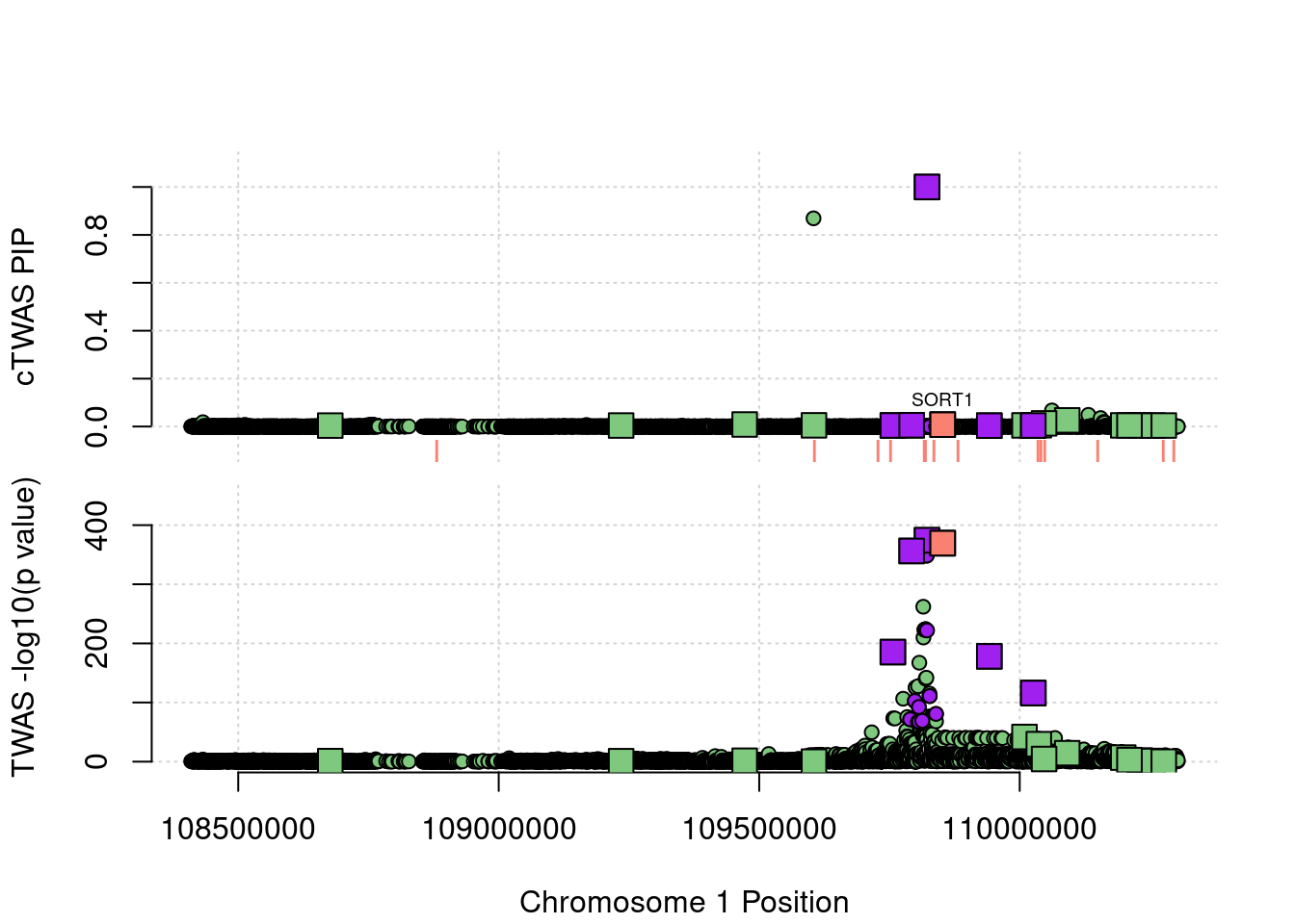
ctwas_gene_res[ctwas_gene_res$region_tag=="1_1", report_cols] genename region_tag susie_pip mu2 PVE z
317 SARS 1_1 0.004441759 829.133716 1.071766e-05 -29.0877047
326 GNAI3 1_1 0.025707252 75.896164 5.678005e-06 -7.8291741
313 SLC25A24 1_1 0.003935600 7.492937 8.581897e-08 -1.4897950
334 KCNC4 1_1 0.007468828 10.219142 2.221197e-07 -0.2619940
315 CLCC1 1_1 0.008596233 15.417625 3.856967e-07 2.1843750
329 GSTM1 1_1 0.005013565 12.168234 1.775393e-07 2.5177822
314 PRPF38B 1_1 0.004235734 7.231967 8.914675e-08 -1.3966706
330 GSTM5 1_1 0.003943466 8.148652 9.351563e-08 1.7854731
331 GSTM3 1_1 0.004373009 6.390789 8.133083e-08 -0.1964803
312 VAV3 1_1 0.005347030 8.804403 1.370039e-07 -1.2082161
319 PSRC1 1_1 0.999997827 1666.665441 4.850291e-03 -41.4304787
320 SORT1 1_1 0.007802750 1643.365355 3.731660e-05 -41.1531241
322 SYPL2 1_1 0.004751791 189.831658 2.625102e-06 -13.6525775
333 STRIP1 1_1 0.009349678 23.742624 6.460196e-07 -3.5645426
321 PSMA5 1_1 0.003803929 793.060734 8.779285e-06 -28.5111708
318 CELSR2 1_1 0.005329615 1584.481288 2.457555e-05 -40.4093624
323 ATXN7L2 1_1 0.004368213 526.198142 6.689188e-06 -22.9669679
327 GSTM4 1_1 0.004807485 31.186871 4.363249e-07 5.2728981
324 CYB561D1 1_1 0.005587258 137.654363 2.238252e-06 11.4426918
325 AMIGO1 1_1 0.013237319 30.817125 1.187169e-06 -4.1691858
332 CSF1 1_1 0.010604946 20.908729 6.452922e-07 -2.7470731
316 TAF13 1_1 0.005033453 7.108649 1.041294e-07 -0.1637351
311 PRMT6 1_1 0.998736063 30.076387 8.741716e-05 -5.1278667
328 GSTM2 1_1 0.004402685 14.107754 1.807573e-07 3.0605130
num_eqtl
317 25
326 5
313 46
334 24
315 34
329 43
314 22
330 67
331 69
312 9
319 15
320 23
322 33
333 6
321 15
318 21
323 34
327 86
324 11
325 10
332 15
316 37
311 21
328 60IRF2BP2/RP4-781K5.7 Locus
This is the locus plot for the IRF2BP2/RP4-781K5.7 locus. IRF2BP2 is the presumed causal gene at this locus, and RP4-781K5.7 is a co-regulated lncRNA. The z score for IRF2BP2 (12.51) is smaller than the z score of RP4-781K5.7 (-14.02). However, both of these genes have PIPs near zero, and SNPs are selected instead. There appear to be several independent signals at this locus, although the exact SNP for each signal is unclear.
locus_plot3("1_2", focus="IRF2BP2")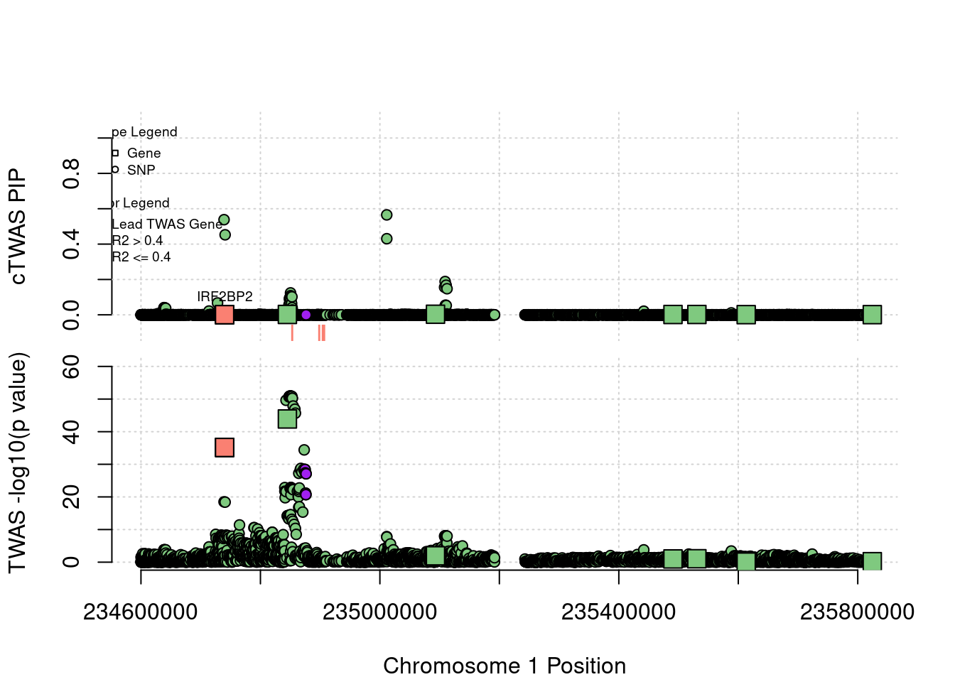
ctwas_gene_res[ctwas_gene_res$region_tag=="1_2", report_cols] genename region_tag susie_pip mu2 PVE
632 GPR137B 1_2 0.0019855648 14.151584 8.177290e-08
629 TBCE 1_2 0.0020044506 15.076420 8.794556e-08
631 LYST 1_2 0.0011613257 7.418435 2.507186e-08
628 GGPS1 1_2 0.0018747050 14.312855 7.808714e-08
630 B3GALNT2 1_2 0.0009645677 6.831947 1.917774e-08
625 IRF2BP2 1_2 0.0008232359 140.988873 3.377765e-07
624 COA6 1_2 0.0011754643 8.423615 2.881564e-08
626 RP4-781K5.7 1_2 0.0022297254 174.926390 1.135081e-06
627 RP11-443B7.1 1_2 0.0033486765 20.433621 1.991310e-07
z num_eqtl
632 1.39195036 45
629 1.69905204 25
631 0.39246189 45
628 1.62972898 7
630 -0.06568788 29
625 12.50646138 6
624 0.33489207 30
626 -14.01515180 7
627 -2.53928509 20
sessionInfo()R version 3.6.1 (2019-07-05)
Platform: x86_64-pc-linux-gnu (64-bit)
Running under: Scientific Linux 7.4 (Nitrogen)
Matrix products: default
BLAS/LAPACK: /software/openblas-0.2.19-el7-x86_64/lib/libopenblas_haswellp-r0.2.19.so
locale:
[1] LC_CTYPE=en_US.UTF-8 LC_NUMERIC=C
[3] LC_TIME=en_US.UTF-8 LC_COLLATE=en_US.UTF-8
[5] LC_MONETARY=en_US.UTF-8 LC_MESSAGES=en_US.UTF-8
[7] LC_PAPER=en_US.UTF-8 LC_NAME=C
[9] LC_ADDRESS=C LC_TELEPHONE=C
[11] LC_MEASUREMENT=en_US.UTF-8 LC_IDENTIFICATION=C
attached base packages:
[1] stats graphics grDevices utils datasets methods base
loaded via a namespace (and not attached):
[1] Rcpp_1.0.6 knitr_1.23 magrittr_2.0.1
[4] workflowr_1.6.2 bit_4.0.4 lattice_0.20-38
[7] R6_2.5.0 rlang_0.4.11 fastmap_1.1.0
[10] stringr_1.4.0 blob_1.2.1 tools_3.6.1
[13] grid_3.6.1 data.table_1.14.0 xfun_0.8
[16] DBI_1.1.1 git2r_0.26.1 htmltools_0.3.6
[19] yaml_2.2.0 bit64_4.0.5 digest_0.6.20
[22] rprojroot_2.0.2 Matrix_1.2-18 later_0.8.0
[25] vctrs_0.3.8 promises_1.0.1 fs_1.3.1
[28] cachem_1.0.5 memoise_2.0.0 glue_1.4.2
[31] evaluate_0.14 RSQLite_2.2.7 rmarkdown_1.13
[34] stringi_1.4.3 compiler_3.6.1 httpuv_1.5.1
[37] pkgconfig_2.0.3