LDL direct (quantile) - Liver
wesleycrouse
2021-09-09
Last updated: 2021-09-09
Checks: 6 1
Knit directory: ctwas_applied/
This reproducible R Markdown analysis was created with workflowr (version 1.6.2). The Checks tab describes the reproducibility checks that were applied when the results were created. The Past versions tab lists the development history.
The R Markdown file has unstaged changes. To know which version of the R Markdown file created these results, you’ll want to first commit it to the Git repo. If you’re still working on the analysis, you can ignore this warning. When you’re finished, you can run wflow_publish to commit the R Markdown file and build the HTML.
Great job! The global environment was empty. Objects defined in the global environment can affect the analysis in your R Markdown file in unknown ways. For reproduciblity it’s best to always run the code in an empty environment.
The command set.seed(20210726) was run prior to running the code in the R Markdown file. Setting a seed ensures that any results that rely on randomness, e.g. subsampling or permutations, are reproducible.
Great job! Recording the operating system, R version, and package versions is critical for reproducibility.
Nice! There were no cached chunks for this analysis, so you can be confident that you successfully produced the results during this run.
Great job! Using relative paths to the files within your workflowr project makes it easier to run your code on other machines.
Great! You are using Git for version control. Tracking code development and connecting the code version to the results is critical for reproducibility.
The results in this page were generated with repository version 59e5f4d. See the Past versions tab to see a history of the changes made to the R Markdown and HTML files.
Note that you need to be careful to ensure that all relevant files for the analysis have been committed to Git prior to generating the results (you can use wflow_publish or wflow_git_commit). workflowr only checks the R Markdown file, but you know if there are other scripts or data files that it depends on. Below is the status of the Git repository when the results were generated:
Unstaged changes:
    Modified:   analysis/ukb-d-30500_irnt_Liver.Rmd
    Modified:   analysis/ukb-d-30600_irnt_Liver.Rmd
    Modified:   analysis/ukb-d-30610_irnt_Liver.Rmd
    Modified:   analysis/ukb-d-30620_irnt_Liver.Rmd
    Modified:   analysis/ukb-d-30630_irnt_Liver.Rmd
    Modified:   analysis/ukb-d-30640_irnt_Liver.Rmd
    Modified:   analysis/ukb-d-30650_irnt_Liver.Rmd
    Modified:   analysis/ukb-d-30660_irnt_Liver.Rmd
    Modified:   analysis/ukb-d-30670_irnt_Liver.Rmd
    Modified:   analysis/ukb-d-30680_irnt_Liver.Rmd
    Modified:   analysis/ukb-d-30690_irnt_Liver.Rmd
    Modified:   analysis/ukb-d-30700_irnt_Liver.Rmd
    Modified:   analysis/ukb-d-30710_irnt_Liver.Rmd
    Modified:   analysis/ukb-d-30720_irnt_Liver.Rmd
    Modified:   analysis/ukb-d-30730_irnt_Liver.Rmd
    Modified:   analysis/ukb-d-30740_irnt_Liver.Rmd
    Modified:   analysis/ukb-d-30750_irnt_Liver.Rmd
    Modified:   analysis/ukb-d-30760_irnt_Liver.Rmd
    Modified:   analysis/ukb-d-30770_irnt_Liver.Rmd
    Modified:   analysis/ukb-d-30780_irnt_Liver.Rmd
Note that any generated files, e.g. HTML, png, CSS, etc., are not included in this status report because it is ok for generated content to have uncommitted changes.
These are the previous versions of the repository in which changes were made to the R Markdown (analysis/ukb-d-30780_irnt_Liver.Rmd) and HTML (docs/ukb-d-30780_irnt_Liver.html) files. If you’ve configured a remote Git repository (see ?wflow_git_remote), click on the hyperlinks in the table below to view the files as they were in that past version.
| File | Version | Author | Date | Message |
|---|---|---|---|---|
| Rmd | cbf7408 | wesleycrouse | 2021-09-08 | adding enrichment to reports |
| html | cbf7408 | wesleycrouse | 2021-09-08 | adding enrichment to reports |
| Rmd | 4970e3e | wesleycrouse | 2021-09-08 | updating reports |
| html | 4970e3e | wesleycrouse | 2021-09-08 | updating reports |
| Rmd | 627a4e1 | wesleycrouse | 2021-09-07 | adding heritability |
| Rmd | dfd2b5f | wesleycrouse | 2021-09-07 | regenerating reports |
| html | dfd2b5f | wesleycrouse | 2021-09-07 | regenerating reports |
| Rmd | 61b53b3 | wesleycrouse | 2021-09-06 | updated PVE calculation |
| html | 61b53b3 | wesleycrouse | 2021-09-06 | updated PVE calculation |
| Rmd | 837dd01 | wesleycrouse | 2021-09-01 | adding additional fixedsigma report |
| Rmd | d0a5417 | wesleycrouse | 2021-08-30 | adding new reports to the index |
| Rmd | 0922de7 | wesleycrouse | 2021-08-18 | updating all reports with locus plots |
| html | 0922de7 | wesleycrouse | 2021-08-18 | updating all reports with locus plots |
| html | 1c62980 | wesleycrouse | 2021-08-11 | Updating reports |
| Rmd | 5981e80 | wesleycrouse | 2021-08-11 | Adding more reports |
| html | 5981e80 | wesleycrouse | 2021-08-11 | Adding more reports |
| Rmd | 05a98b7 | wesleycrouse | 2021-08-07 | adding additional results |
| html | 05a98b7 | wesleycrouse | 2021-08-07 | adding additional results |
| html | 03e541c | wesleycrouse | 2021-07-29 | Cleaning up report generation |
| html | 276893d | wesleycrouse | 2021-07-29 | Updating reports |
| html | 4068e9b | wesleycrouse | 2021-07-29 | finalizing automation |
| Rmd | 0e62fa9 | wesleycrouse | 2021-07-29 | Automating reports |
| html | 0e62fa9 | wesleycrouse | 2021-07-29 | Automating reports |
Overview
These are the results of a ctwas analysis of the UK Biobank trait LDL direct (quantile) using Liver gene weights.
The GWAS was conducted by the Neale Lab, and the biomarker traits we analyzed are discussed here. Summary statistics were obtained from IEU OpenGWAS using GWAS ID: ukb-d-30780_irnt. Results were obtained from from IEU rather than Neale Lab because they are in a standardard format (GWAS VCF). Note that 3 of the 34 biomarker traits were not available from IEU and were excluded from analysis.
The weights are mashr GTEx v8 models on Liver eQTL obtained from PredictDB. We performed a full harmonization of the variants, including recovering strand ambiguous variants. This procedure is discussed in a separate document. (TO-DO: add report that describes harmonization)
LD matrices were computed from a 10% subset of Neale lab subjects. Subjects were matched using the plate and well information from genotyping. We included only biallelic variants with MAF>0.01 in the original Neale Lab GWAS. (TO-DO: add more details [number of subjects, variants, etc])
Weight QC
TO-DO: add enhanced QC reporting (total number of weights, why each variant was missing for all genes)
qclist_all <- list()

qc_files <- paste0(results_dir, "/", list.files(results_dir, pattern="exprqc.Rd"))

for (i in 1:length(qc_files)){
  load(qc_files[i])
  chr <- unlist(strsplit(rev(unlist(strsplit(qc_files[i], "_")))[1], "[.]"))[1]
  qclist_all[[chr]] <- cbind(do.call(rbind, lapply(qclist,unlist)), as.numeric(substring(chr,4)))
}

qclist_all <- data.frame(do.call(rbind, qclist_all))
colnames(qclist_all)[ncol(qclist_all)] <- "chr"

rm(qclist, wgtlist, z_gene_chr)

#number of imputed weights
nrow(qclist_all)
[1] 10901#number of imputed weights by chromosome
table(qclist_all$chr)
   1    2    3    4    5    6    7    8    9   10   11   12   13   14   15
1070  768  652  417  494  611  548  408  405  434  634  629  195  365  354
  16   17   18   19   20   21   22
 526  663  160  859  306  114  289
#proportion of imputed weights without missing variants
mean(qclist_all$nmiss==0)[1] 0.8366205Load ctwas results
#load ctwas results
ctwas_res <- data.table::fread(paste0(results_dir, "/", analysis_id, "_ctwas.susieIrss.txt"))

#make unique identifier for regions
ctwas_res$region_tag <- paste(ctwas_res$region_tag1, ctwas_res$region_tag2, sep="_")

#compute PVE for each gene/SNP
ctwas_res$PVE = ctwas_res$susie_pip*ctwas_res$mu2/sample_size #check PVE calculation

#separate gene and SNP results
ctwas_gene_res <- ctwas_res[ctwas_res$type == "gene", ]
ctwas_gene_res <- data.frame(ctwas_gene_res)
ctwas_snp_res <- ctwas_res[ctwas_res$type == "SNP", ]
ctwas_snp_res <- data.frame(ctwas_snp_res)

#add gene information to results
sqlite <- RSQLite::dbDriver("SQLite")
db = RSQLite::dbConnect(sqlite, paste0("/project2/compbio/predictdb/mashr_models/mashr_", weight, ".db"))
query <- function(...) RSQLite::dbGetQuery(db, ...)
gene_info <- query("select gene, genename from extra")
gene_info <- query("select gene, genename, gene_type from extra")
RSQLite::dbDisconnect(db)

ctwas_gene_res <- cbind(ctwas_gene_res, gene_info[sapply(ctwas_gene_res$id, match, gene_info$gene), c("genename", "gene_type")])

#add z score to results
load(paste0(results_dir, "/", analysis_id, "_expr_z_gene.Rd"))
ctwas_gene_res$z <- z_gene[ctwas_gene_res$id,]$z

#load(paste0(results_dir, "/", analysis_id, "_expr_z_snp.Rd")) #for new version, stored after harmonization
z_snp <- readRDS(paste0(results_dir, "/", trait_id, ".RDS")) #for old version, unharmonized

z_snp <- z_snp[z_snp$id %in% ctwas_snp_res$id,] #subset snps to those included in analysis, note some are duplicated, need to match which allele was used
ctwas_snp_res$z <- z_snp$z[match(ctwas_snp_res$id, z_snp$id)] #for duplicated snps, this arbitrarily uses the first allele
ctwas_snp_res$z_flag <- as.numeric(ctwas_snp_res$id %in% z_snp$id[duplicated(z_snp$id)]) #mark the unclear z scores, flag=1

#formatting and rounding for tables
ctwas_gene_res$z <- round(ctwas_gene_res$z,2)
ctwas_snp_res$z <- round(ctwas_snp_res$z,2)
ctwas_gene_res$susie_pip <- round(ctwas_gene_res$susie_pip,3)
ctwas_snp_res$susie_pip <- round(ctwas_snp_res$susie_pip,3)
ctwas_gene_res$mu2 <- round(ctwas_gene_res$mu2,2)
ctwas_snp_res$mu2 <- round(ctwas_snp_res$mu2,2)
ctwas_gene_res$PVE <- signif(ctwas_gene_res$PVE, 2)
ctwas_snp_res$PVE <- signif(ctwas_snp_res$PVE, 2)

#merge gene and snp results with added information
ctwas_gene_res$z_flag=NA
ctwas_snp_res$genename=NA
ctwas_snp_res$gene_type=NA

ctwas_res <- rbind(ctwas_gene_res,
                   ctwas_snp_res[,colnames(ctwas_gene_res)])

#store columns to report
report_cols <- colnames(ctwas_gene_res)[!(colnames(ctwas_gene_res) %in% c("type", "region_tag1", "region_tag2", "cs_index", "gene_type", "z_flag", "id", "chrom", "pos"))]
first_cols <- c("genename", "region_tag")
report_cols <- c(first_cols, report_cols[!(report_cols %in% first_cols)])

report_cols_snps <- c("id", report_cols[-1])

#get number of SNPs from s1 results; adjust for thin
ctwas_res_s1 <- data.table::fread(paste0(results_dir, "/", analysis_id, "_ctwas.s1.susieIrss.txt"))
n_snps <- sum(ctwas_res_s1$type=="SNP")/thin
rm(ctwas_res_s1)
Check convergence of parameters
library(ggplot2)
library(cowplot)
********************************************************Note: As of version 1.0.0, cowplot does not change the default ggplot2 theme anymore. To recover the previous behavior, execute:
theme_set(theme_cowplot())********************************************************load(paste0(results_dir, "/", analysis_id, "_ctwas.s2.susieIrssres.Rd"))
df <- data.frame(niter = rep(1:ncol(group_prior_rec), 2),
value = c(group_prior_rec[1,], group_prior_rec[2,]),
group = rep(c("Gene", "SNP"), each = ncol(group_prior_rec)))
df$group <- as.factor(df$group)
df$value[df$group=="SNP"] <- df$value[df$group=="SNP"]*thin #adjust parameter to account for thin argument
p_pi <- ggplot(df, aes(x=niter, y=value, group=group)) +
geom_line(aes(color=group)) +
geom_point(aes(color=group)) +
xlab("Iteration") + ylab(bquote(pi)) +
ggtitle("Prior mean") +
theme_cowplot()
df <- data.frame(niter = rep(1:ncol(group_prior_var_rec), 2),
value = c(group_prior_var_rec[1,], group_prior_var_rec[2,]),
group = rep(c("Gene", "SNP"), each = ncol(group_prior_var_rec)))
df$group <- as.factor(df$group)
p_sigma2 <- ggplot(df, aes(x=niter, y=value, group=group)) +
geom_line(aes(color=group)) +
geom_point(aes(color=group)) +
xlab("Iteration") + ylab(bquote(sigma^2)) +
ggtitle("Prior variance") +
theme_cowplot()
plot_grid(p_pi, p_sigma2)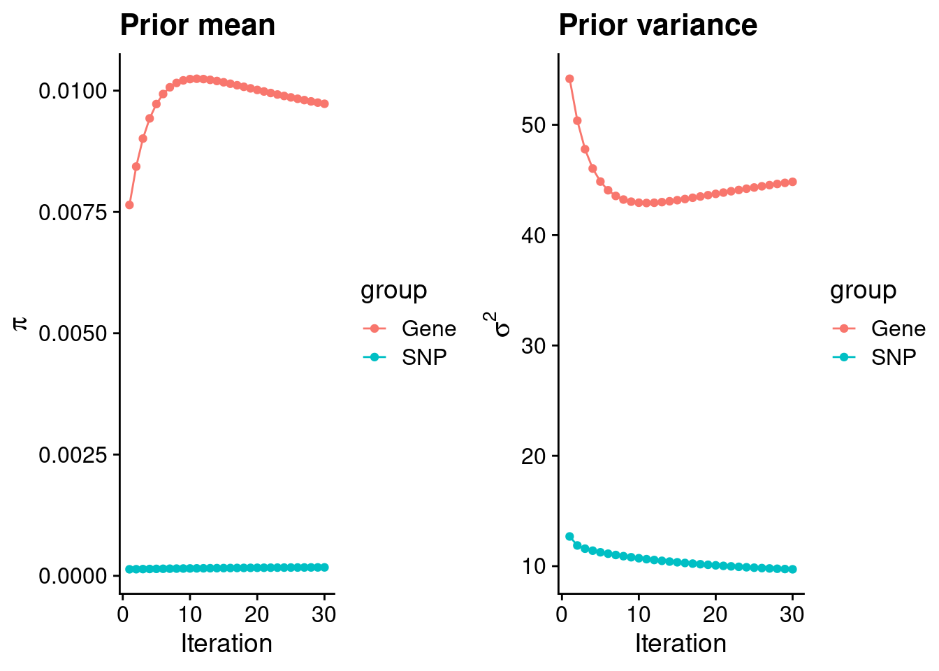
#estimated group prior
estimated_group_prior <- group_prior_rec[,ncol(group_prior_rec)]
names(estimated_group_prior) <- c("gene", "snp")
estimated_group_prior["snp"] <- estimated_group_prior["snp"]*thin #adjust parameter to account for thin argument
print(estimated_group_prior)
gene snp
0.0097295269 0.0001740615 #estimated group prior variance
estimated_group_prior_var <- group_prior_var_rec[,ncol(group_prior_var_rec)]
names(estimated_group_prior_var) <- c("gene", "snp")
print(estimated_group_prior_var) gene snp
44.830537 9.714877 #report sample size
print(sample_size)[1] 343621#report group size
group_size <- c(nrow(ctwas_gene_res), n_snps)
print(group_size)[1] 10901 8697330#estimated group PVE
estimated_group_pve <- estimated_group_prior_var*estimated_group_prior*group_size/sample_size #check PVE calculation
names(estimated_group_pve) <- c("gene", "snp")
print(estimated_group_pve) gene snp
0.01383733 0.04280025 #compare sum(PIP*mu2/sample_size) with above PVE calculation
c(sum(ctwas_gene_res$PVE),sum(ctwas_snp_res$PVE))[1] 0.02598409 0.37522284Genes with highest PIPs
#distribution of PIPs
hist(ctwas_gene_res$susie_pip, xlim=c(0,1), main="Distribution of Gene PIPs")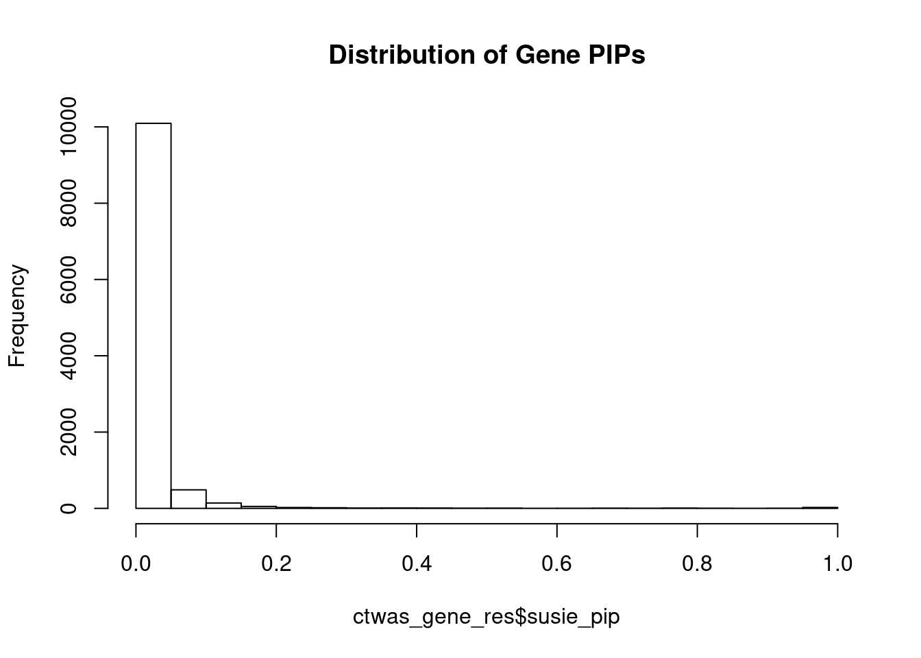
#genes with PIP>0.8 or 20 highest PIPs
head(ctwas_gene_res[order(-ctwas_gene_res$susie_pip),report_cols], max(sum(ctwas_gene_res$susie_pip>0.8), 20))
genename region_tag susie_pip mu2 PVE z
4435 PSRC1 1_67 1.000 1673.70 4.9e-03 -41.69
5544 CNIH4 1_114 1.000 48.38 1.4e-04 6.72
12687 RP4-781K5.7 1_121 1.000 203.72 5.9e-04 -15.11
5563 ABCG8 2_27 1.000 313.63 9.1e-04 -20.29
3721 INSIG2 2_69 1.000 159.89 4.7e-04 -9.36
5991 FADS1 11_34 1.000 160.59 4.7e-04 12.83
12008 HPR 16_38 1.000 209.85 6.1e-04 -17.24
10657 TRIM39 6_24 0.999 72.25 2.1e-04 8.85
1999 PRKD2 19_33 0.996 32.48 9.4e-05 5.29
7410 ABCA1 9_53 0.995 70.37 2.0e-04 7.98
9390 GAS6 13_62 0.988 71.36 2.1e-04 -8.92
1597 PLTP 20_28 0.988 61.57 1.8e-04 -5.73
8531 TNKS 8_12 0.984 73.77 2.1e-04 11.03
7040 INHBB 2_70 0.982 74.05 2.1e-04 -8.52
2092 SP4 7_19 0.977 102.39 2.9e-04 10.69
6093 CSNK1G3 5_75 0.975 84.23 2.4e-04 9.12
4704 DDX56 7_32 0.975 58.70 1.7e-04 9.45
6996 ACP6 1_73 0.969 25.68 7.2e-05 4.65
6220 PELO 5_31 0.967 72.15 2.0e-04 8.43
8865 FUT2 19_33 0.965 104.79 2.9e-04 -11.93
233 NPC1L1 7_32 0.964 89.80 2.5e-04 -10.76
11790 CYP2A6 19_28 0.962 32.01 9.0e-05 5.41
3247 KDSR 18_35 0.955 24.69 6.9e-05 -4.53
3562 ACVR1C 2_94 0.939 26.34 7.2e-05 -4.74
6778 PKN3 9_66 0.936 47.71 1.3e-04 -6.62
1114 SRRT 7_62 0.927 33.01 8.9e-05 5.55
6391 TTC39B 9_13 0.926 23.05 6.2e-05 -4.29
6957 USP1 1_39 0.894 253.89 6.6e-04 16.26
3300 C10orf88 10_77 0.880 35.78 9.2e-05 -6.63
9062 KLHDC7A 1_13 0.818 22.60 5.4e-05 4.12
9072 SPTY2D1 11_13 0.810 33.54 7.9e-05 -5.56
8931 CRACR2B 11_1 0.802 22.04 5.1e-05 -3.99
8418 POP7 7_62 0.801 40.08 9.3e-05 -5.85Genes with largest effect sizes
#plot PIP vs effect size
plot(ctwas_gene_res$susie_pip, ctwas_gene_res$mu2, xlab="PIP", ylab="mu^2", main="Gene PIPs vs Effect Size")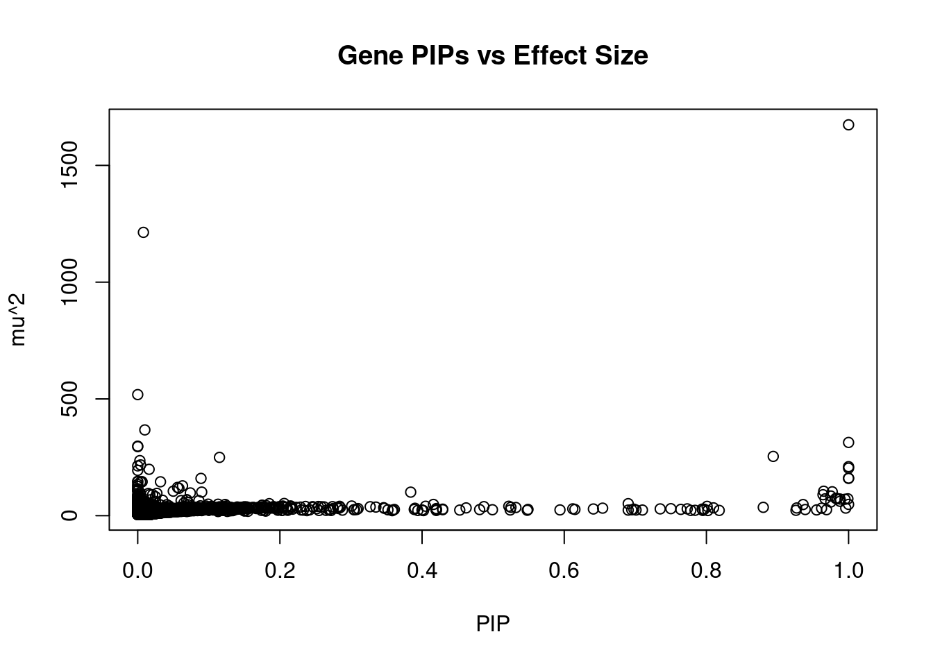
#genes with 20 largest effect sizes
head(ctwas_gene_res[order(-ctwas_gene_res$mu2),report_cols],20)
genename region_tag susie_pip mu2 PVE z
4435 PSRC1 1_67 1.000 1673.70 4.9e-03 -41.69
5436 PSMA5 1_67 0.008 1213.20 2.8e-05 -35.41
4562 SRPK2 7_65 0.000 518.50 0.0e+00 -1.46
6970 ATXN7L2 1_67 0.010 367.29 1.1e-05 -19.24
5563 ABCG8 2_27 1.000 313.63 9.1e-04 -20.29
11364 RP11-325F22.2 7_65 0.000 297.63 0.0e+00 0.97
781 PVR 19_32 0.000 295.71 0.0e+00 -10.08
6957 USP1 1_39 0.894 253.89 6.6e-04 16.26
4317 ANGPTL3 1_39 0.115 249.66 8.4e-05 16.13
11684 RP11-136O12.2 8_83 0.003 235.91 2.1e-06 14.40
3441 POLK 5_45 0.004 217.46 2.6e-06 17.52
11108 AC093901.1 2_69 0.000 213.31 0.0e+00 2.46
12008 HPR 16_38 1.000 209.85 6.1e-04 -17.24
12687 RP4-781K5.7 1_121 1.000 203.72 5.9e-04 -15.11
5431 SYPL2 1_67 0.016 198.61 9.5e-06 -14.15
5377 GEMIN7 19_32 0.000 193.98 0.0e+00 10.94
5991 FADS1 11_34 1.000 160.59 4.7e-04 12.83
3721 INSIG2 2_69 1.000 159.89 4.7e-04 -9.36
5240 NLRC5 16_31 0.089 159.69 4.1e-05 11.86
538 ZNF112 19_32 0.000 147.06 0.0e+00 10.39Genes with highest PVE
#genes with 20 highest pve
head(ctwas_gene_res[order(-ctwas_gene_res$PVE),report_cols],20)
genename region_tag susie_pip mu2 PVE z
4435 PSRC1 1_67 1.000 1673.70 0.00490 -41.69
5563 ABCG8 2_27 1.000 313.63 0.00091 -20.29
6957 USP1 1_39 0.894 253.89 0.00066 16.26
12008 HPR 16_38 1.000 209.85 0.00061 -17.24
12687 RP4-781K5.7 1_121 1.000 203.72 0.00059 -15.11
3721 INSIG2 2_69 1.000 159.89 0.00047 -9.36
5991 FADS1 11_34 1.000 160.59 0.00047 12.83
2092 SP4 7_19 0.977 102.39 0.00029 10.69
8865 FUT2 19_33 0.965 104.79 0.00029 -11.93
233 NPC1L1 7_32 0.964 89.80 0.00025 -10.76
6093 CSNK1G3 5_75 0.975 84.23 0.00024 9.12
7040 INHBB 2_70 0.982 74.05 0.00021 -8.52
10657 TRIM39 6_24 0.999 72.25 0.00021 8.85
8531 TNKS 8_12 0.984 73.77 0.00021 11.03
9390 GAS6 13_62 0.988 71.36 0.00021 -8.92
6220 PELO 5_31 0.967 72.15 0.00020 8.43
7410 ABCA1 9_53 0.995 70.37 0.00020 7.98
1597 PLTP 20_28 0.988 61.57 0.00018 -5.73
4704 DDX56 7_32 0.975 58.70 0.00017 9.45
5544 CNIH4 1_114 1.000 48.38 0.00014 6.72Genes with largest z scores
#genes with 20 largest z scores
head(ctwas_gene_res[order(-abs(ctwas_gene_res$z)),report_cols],20)
genename region_tag susie_pip mu2 PVE z
4435 PSRC1 1_67 1.000 1673.70 4.9e-03 -41.69
5436 PSMA5 1_67 0.008 1213.20 2.8e-05 -35.41
5563 ABCG8 2_27 1.000 313.63 9.1e-04 -20.29
6970 ATXN7L2 1_67 0.010 367.29 1.1e-05 -19.24
3441 POLK 5_45 0.004 217.46 2.6e-06 17.52
12008 HPR 16_38 1.000 209.85 6.1e-04 -17.24
6957 USP1 1_39 0.894 253.89 6.6e-04 16.26
4317 ANGPTL3 1_39 0.115 249.66 8.4e-05 16.13
12687 RP4-781K5.7 1_121 1.000 203.72 5.9e-04 -15.11
9978 ANKDD1B 5_45 0.004 144.63 1.7e-06 15.07
11684 RP11-136O12.2 8_83 0.003 235.91 2.1e-06 14.40
5431 SYPL2 1_67 0.016 198.61 9.5e-06 -14.15
1930 PPP1R37 19_32 0.000 125.33 0.0e+00 -12.89
5991 FADS1 11_34 1.000 160.59 4.7e-04 12.83
4507 FADS2 11_34 0.006 145.20 2.7e-06 12.07
7955 FEN1 11_34 0.006 145.20 2.7e-06 12.07
4112 YIPF2 19_9 0.000 126.57 8.1e-13 11.94
8865 FUT2 19_33 0.965 104.79 2.9e-04 -11.93
5240 NLRC5 16_31 0.089 159.69 4.1e-05 11.86
1053 APOB 2_13 0.000 62.93 3.0e-15 -11.73Comparing z scores and PIPs
#set nominal signifiance threshold for z scores
alpha <- 0.05

#bonferroni adjusted threshold for z scores
sig_thresh <- qnorm(1-(alpha/nrow(ctwas_gene_res)/2), lower=T)

#Q-Q plot for z scores
obs_z <- ctwas_gene_res$z[order(ctwas_gene_res$z)]
exp_z <- qnorm((1:nrow(ctwas_gene_res))/nrow(ctwas_gene_res))

plot(exp_z, obs_z, xlab="Expected z", ylab="Observed z", main="Gene z score Q-Q plot")
abline(a=0,b=1)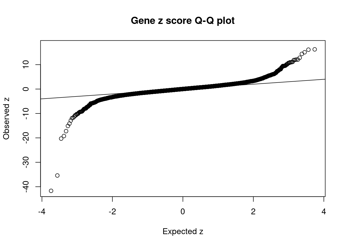
| Version | Author | Date |
|---|---|---|
| dfd2b5f | wesleycrouse | 2021-09-07 |
#plot z score vs PIP
plot(abs(ctwas_gene_res$z), ctwas_gene_res$susie_pip, xlab="abs(z)", ylab="PIP")
abline(v=sig_thresh, col="red", lty=2)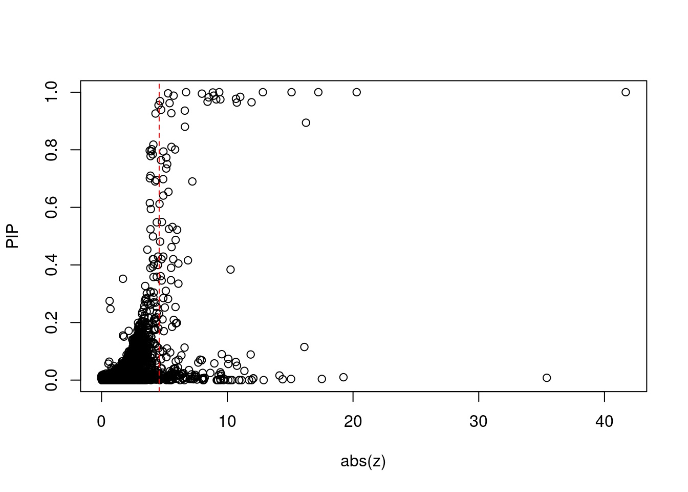
| Version | Author | Date |
|---|---|---|
| dfd2b5f | wesleycrouse | 2021-09-07 |
#proportion of significant z scores
mean(abs(ctwas_gene_res$z) > sig_thresh)
[1] 0.01972296#genes with most significant z scores
head(ctwas_gene_res[order(-abs(ctwas_gene_res$z)),report_cols],20) genename region_tag susie_pip mu2 PVE z
4435 PSRC1 1_67 1.000 1673.70 4.9e-03 -41.69
5436 PSMA5 1_67 0.008 1213.20 2.8e-05 -35.41
5563 ABCG8 2_27 1.000 313.63 9.1e-04 -20.29
6970 ATXN7L2 1_67 0.010 367.29 1.1e-05 -19.24
3441 POLK 5_45 0.004 217.46 2.6e-06 17.52
12008 HPR 16_38 1.000 209.85 6.1e-04 -17.24
6957 USP1 1_39 0.894 253.89 6.6e-04 16.26
4317 ANGPTL3 1_39 0.115 249.66 8.4e-05 16.13
12687 RP4-781K5.7 1_121 1.000 203.72 5.9e-04 -15.11
9978 ANKDD1B 5_45 0.004 144.63 1.7e-06 15.07
11684 RP11-136O12.2 8_83 0.003 235.91 2.1e-06 14.40
5431 SYPL2 1_67 0.016 198.61 9.5e-06 -14.15
1930 PPP1R37 19_32 0.000 125.33 0.0e+00 -12.89
5991 FADS1 11_34 1.000 160.59 4.7e-04 12.83
4507 FADS2 11_34 0.006 145.20 2.7e-06 12.07
7955 FEN1 11_34 0.006 145.20 2.7e-06 12.07
4112 YIPF2 19_9 0.000 126.57 8.1e-13 11.94
8865 FUT2 19_33 0.965 104.79 2.9e-04 -11.93
5240 NLRC5 16_31 0.089 159.69 4.1e-05 11.86
1053 APOB 2_13 0.000 62.93 3.0e-15 -11.73Locus plots for genes and SNPs
ctwas_gene_res_sortz <- ctwas_gene_res[order(-abs(ctwas_gene_res$z)),]

n_plots <- 5
for (region_tag_plot in head(unique(ctwas_gene_res_sortz$region_tag), n_plots)){
  ctwas_res_region <-  ctwas_res[ctwas_res$region_tag==region_tag_plot,]
  start <- min(ctwas_res_region$pos)
  end <- max(ctwas_res_region$pos)

  ctwas_res_region <- ctwas_res_region[order(ctwas_res_region$pos),]
  ctwas_res_region_gene <- ctwas_res_region[ctwas_res_region$type=="gene",]
  ctwas_res_region_snp <- ctwas_res_region[ctwas_res_region$type=="SNP",]

  #region name
  print(paste0("Region: ", region_tag_plot))

  #table of genes in region
  print(ctwas_res_region_gene[,report_cols])

  par(mfrow=c(4,1))

  #gene z scores
  plot(ctwas_res_region_gene$pos, abs(ctwas_res_region_gene$z), xlab="Position", ylab="abs(gene_z)", xlim=c(start,end),
   ylim=c(0,max(sig_thresh, abs(ctwas_res_region_gene$z))),
   main=paste0("Region: ", region_tag_plot))
  abline(h=sig_thresh,col="red",lty=2)

  #significance threshold for SNPs
  alpha_snp <- 5*10^(-8)
  sig_thresh_snp <- qnorm(1-alpha_snp/2, lower=T)

  #snp z scores
  plot(ctwas_res_region_snp$pos, abs(ctwas_res_region_snp$z), xlab="Position", ylab="abs(snp_z)",xlim=c(start,end),
   ylim=c(0,max(sig_thresh_snp, max(abs(ctwas_res_region_snp$z)))))
  abline(h=sig_thresh_snp,col="purple",lty=2)

  #gene pips
  plot(ctwas_res_region_gene$pos, ctwas_res_region_gene$susie_pip, xlab="Position", ylab="Gene PIP", xlim=c(start,end), ylim=c(0,1))
  abline(h=0.8,col="blue",lty=2)

  #snp pips
  plot(ctwas_res_region_snp$pos, ctwas_res_region_snp$susie_pip, xlab="Position", ylab="SNP PIP", xlim=c(start,end), ylim=c(0,1))
  abline(h=0.8,col="blue",lty=2)
}
[1] "Region: 1_67"
genename region_tag susie_pip mu2 PVE z
4434 VAV3 1_67 0.064 24.21 4.5e-06 -2.10
1073 SLC25A24 1_67 0.009 6.52 1.7e-07 0.92
6966 FAM102B 1_67 0.008 6.08 1.4e-07 -1.14
3009 STXBP3 1_67 0.018 18.59 9.6e-07 3.00
3438 GPSM2 1_67 0.008 9.04 2.1e-07 -1.93
3437 CLCC1 1_67 0.008 11.38 2.7e-07 2.57
10286 TAF13 1_67 0.011 9.58 3.1e-07 -1.56
10955 TMEM167B 1_67 0.013 10.96 4.2e-07 -1.53
315 SARS 1_67 0.015 95.12 4.1e-06 9.52
5431 SYPL2 1_67 0.016 198.61 9.5e-06 -14.15
5436 PSMA5 1_67 0.008 1213.20 2.8e-05 -35.41
6970 ATXN7L2 1_67 0.010 367.29 1.1e-05 -19.24
4435 PSRC1 1_67 1.000 1673.70 4.9e-03 -41.69
8615 CYB561D1 1_67 0.063 127.86 2.3e-05 10.68
9259 AMIGO1 1_67 0.019 27.96 1.5e-06 -3.96
6445 GPR61 1_67 0.008 23.02 5.3e-07 4.24
587 GNAI3 1_67 0.052 31.40 4.7e-06 -3.84
7977 GSTM4 1_67 0.015 30.94 1.3e-06 4.78
10821 GSTM2 1_67 0.009 14.30 3.6e-07 2.97
4430 GSTM1 1_67 0.019 29.06 1.6e-06 4.26
4432 GSTM5 1_67 0.014 14.94 6.3e-07 2.38
4433 GSTM3 1_67 0.008 20.94 4.8e-07 -3.95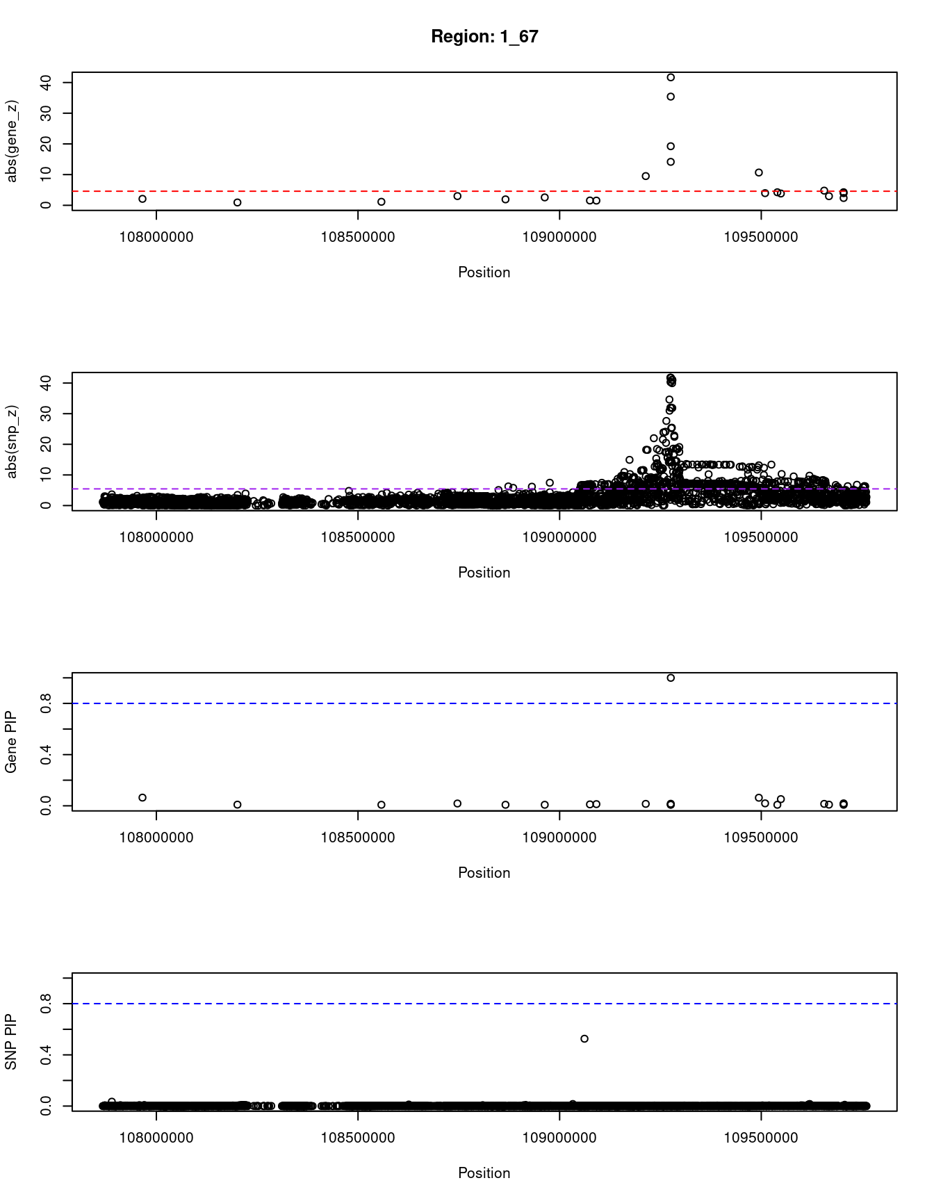
| Version | Author | Date |
|---|---|---|
| dfd2b5f | wesleycrouse | 2021-09-07 |
[1] "Region: 2_27"
        genename region_tag susie_pip    mu2     PVE      z
12661  LINC01126       2_27         0  17.79 6.8e-10   0.92
2977       THADA       2_27         0   8.19 4.2e-11  -2.35
6208     PLEKHH2       2_27         0  16.11 3.0e-10  -2.96
11022 C1GALT1C1L       2_27         0  24.31 2.8e-10   3.06
4930    DYNC2LI1       2_27         0   8.22 2.1e-11  -0.03
5563       ABCG8       2_27         1 313.63 9.1e-04 -20.29
4943      LRPPRC       2_27         0  12.55 9.3e-11  -0.92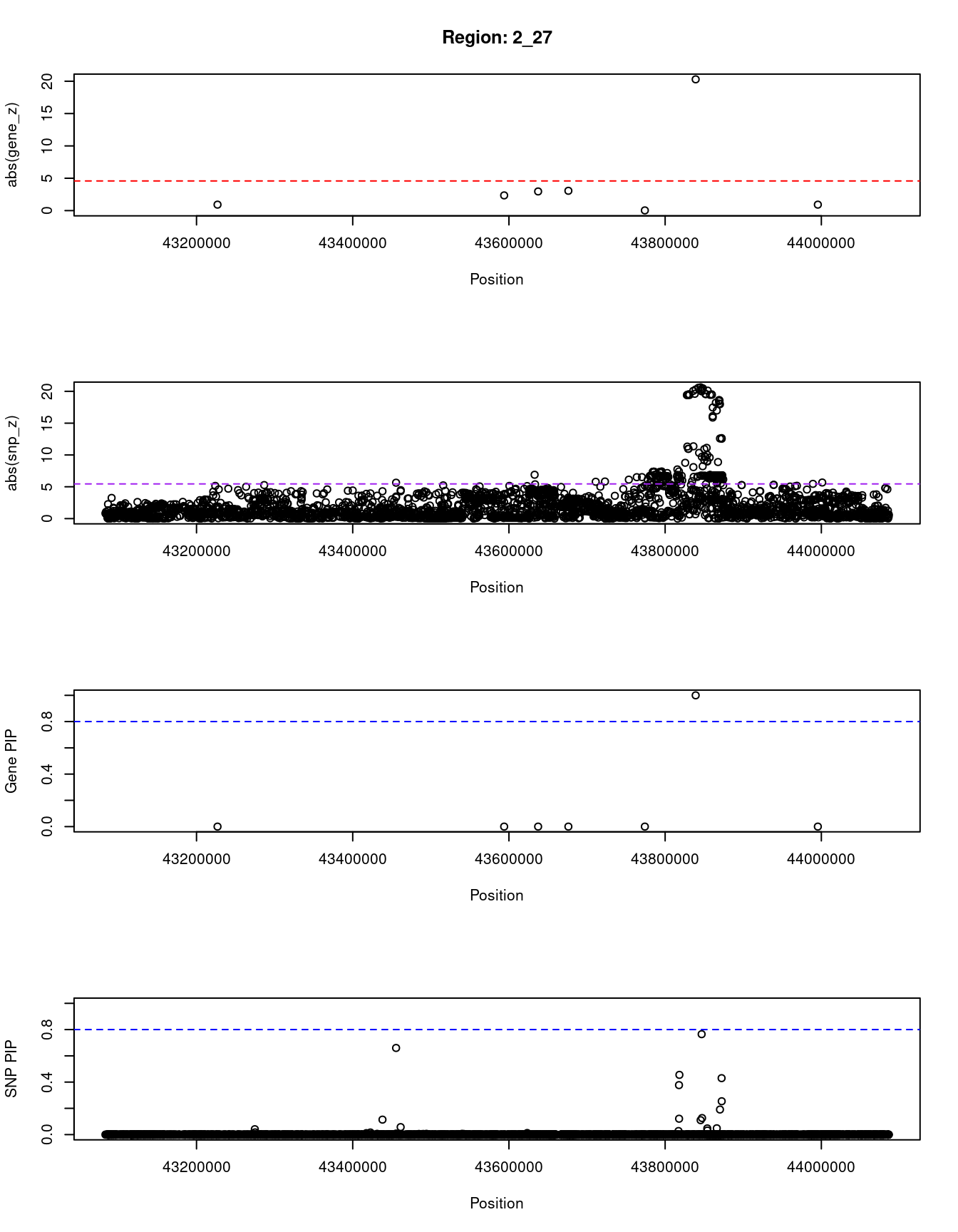
| Version | Author | Date |
|---|---|---|
| dfd2b5f | wesleycrouse | 2021-09-07 |
[1] "Region: 5_45"
          genename region_tag susie_pip    mu2     PVE      z
8340          ENC1       5_45     0.001   5.04 1.5e-08  -0.40
7307          GFM2       5_45     0.001   6.98 2.7e-08  -0.41
7306          NSA2       5_45     0.003  15.65 1.2e-07  -2.05
10458      FAM169A       5_45     0.001   6.14 2.0e-08  -0.98
3441          POLK       5_45     0.004 217.46 2.6e-06  17.52
12287 CTC-366B18.4       5_45     0.050 104.95 1.5e-05 -10.77
9978       ANKDD1B       5_45     0.004 144.63 1.7e-06  15.07
6186          POC5       5_45     0.004  49.43 5.8e-07  -7.01
11757   AC113404.1       5_45     0.002  13.68 7.1e-08   2.33
5717        IQGAP2       5_45     0.006  22.93 3.7e-07   2.57
7281         F2RL2       5_45     0.001   6.62 2.4e-08   0.59
9219           F2R       5_45     0.002  11.37 6.7e-08  -1.21
7287         F2RL1       5_45     0.011  27.62 8.9e-07   2.25
5718         CRHBP       5_45     0.001   6.62 2.4e-08  -0.63
7288         AGGF1       5_45     0.001   6.09 2.1e-08  -0.51
4314         ZBED3       5_45     0.006  21.53 3.5e-07  -1.88
2729         PDE8B       5_45     0.001   5.78 1.9e-08   0.44
7289         WDR41       5_45     0.001   5.65 1.8e-08  -0.41
4313         AP3B1       5_45     0.004  18.48 2.2e-07   1.71
| Version | Author | Date |
|---|---|---|
| dfd2b5f | wesleycrouse | 2021-09-07 |
[1] "Region: 16_38"
      genename region_tag susie_pip    mu2     PVE      z
9196     CMTR2      16_38     0.005  17.93 2.8e-07   3.14
5237     CHST4      16_38     0.002  13.04 8.5e-08   5.64
7757     ZNF23      16_38     0.003  14.10 1.1e-07  -2.84
6535     ZNF19      16_38     0.006  22.58 4.1e-07  -1.74
10432      TAT      16_38     0.002  22.40 1.6e-07   5.47
5236  MARVELD3      16_38     0.003  21.35 1.9e-07  -2.08
366     PHLPP2      16_38     0.005  51.93 7.7e-07  -7.22
11042   ATXN1L      16_38     0.002  56.93 3.8e-07  -8.13
1752    ZNF821      16_38     0.002  46.15 3.1e-07   7.59
12612   PKD1L3      16_38     0.003  99.19 9.5e-07   5.00
12008      HPR      16_38     1.000 209.85 6.1e-04 -17.24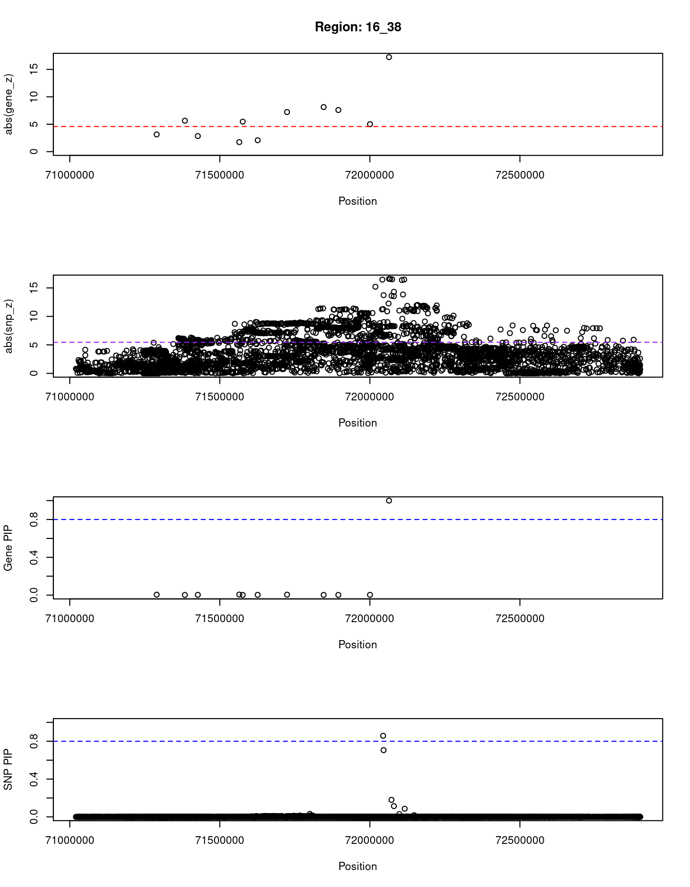
| Version | Author | Date |
|---|---|---|
| dfd2b5f | wesleycrouse | 2021-09-07 |
[1] "Region: 1_39"
     genename region_tag susie_pip    mu2     PVE     z
6956    TM2D1       1_39     0.057  23.07 3.8e-06  2.14
4316    KANK4       1_39     0.009   5.08 1.3e-07  0.51
6957     USP1       1_39     0.894 253.89 6.6e-04 16.26
4317  ANGPTL3       1_39     0.115 249.66 8.4e-05 16.13
3024    DOCK7       1_39     0.010  24.34 7.1e-07  4.46
3733    ATG4C       1_39     0.025  81.35 5.9e-06 -8.65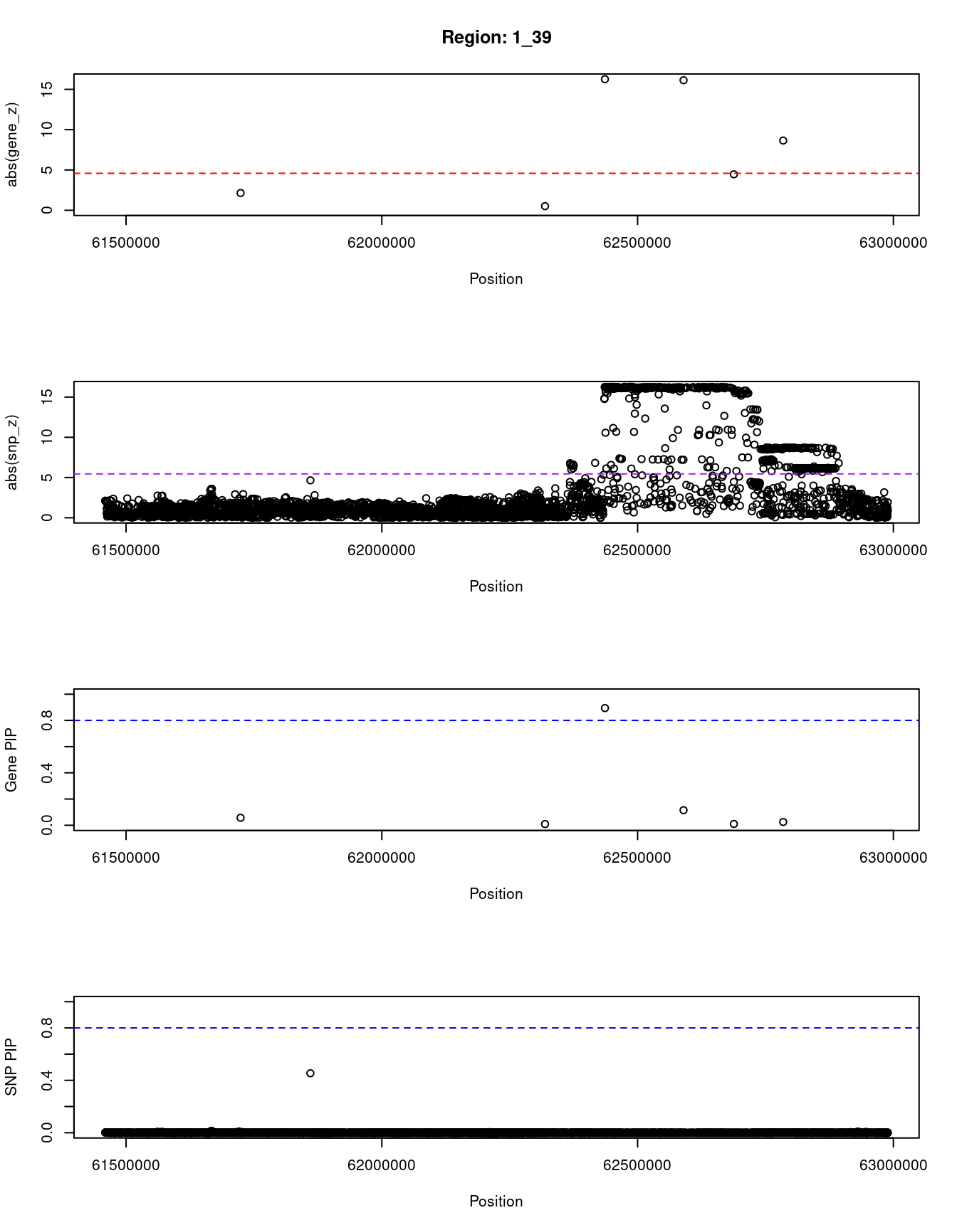
| Version | Author | Date |
|---|---|---|
| dfd2b5f | wesleycrouse | 2021-09-07 |
SNPs with highest PIPs
#snps with PIP>0.8 or 20 highest PIPs
head(ctwas_snp_res[order(-ctwas_snp_res$susie_pip),report_cols_snps],
max(sum(ctwas_snp_res$susie_pip>0.8), 20))
id region_tag susie_pip mu2 PVE z
7471 rs79598313 1_18 1.000 46.26 1.3e-04 7.02
13985 rs11580527 1_34 1.000 87.74 2.6e-04 -11.17
14015 rs2495502 1_34 1.000 283.40 8.2e-04 6.29
14026 rs10888896 1_34 1.000 131.45 3.8e-04 11.89
14033 rs471705 1_34 1.000 207.62 6.0e-04 16.26
52934 rs2807848 1_112 1.000 58.52 1.7e-04 -7.88
67958 rs11679386 2_12 1.000 127.41 3.7e-04 11.91
68007 rs1042034 2_13 1.000 233.16 6.8e-04 16.57
68013 rs934197 2_13 1.000 415.42 1.2e-03 33.06
68016 rs548145 2_13 1.000 656.38 1.9e-03 33.09
68093 rs1848922 2_13 1.000 229.86 6.7e-04 25.41
69743 rs780093 2_16 1.000 160.70 4.7e-04 -14.14
75421 rs72800939 2_28 1.000 55.14 1.6e-04 -7.85
159815 rs768688512 3_58 1.000 299.22 8.7e-04 2.62
317904 rs11376017 6_13 1.000 64.30 1.9e-04 -8.51
347121 rs9496567 6_67 1.000 38.27 1.1e-04 -6.34
365688 rs12208357 6_103 1.000 234.69 6.8e-04 12.28
365872 rs56393506 6_104 1.000 88.87 2.6e-04 14.09
402338 rs763798411 7_65 1.000 3396.95 9.9e-03 -3.27
438749 rs140753685 8_42 1.000 54.27 1.6e-04 7.80
440145 rs4738679 8_45 1.000 106.62 3.1e-04 -11.70
459808 rs13252684 8_83 1.000 216.75 6.3e-04 11.96
500347 rs115478735 9_70 1.000 302.07 8.8e-04 19.01
582983 rs4937122 11_77 1.000 77.07 2.2e-04 12.15
752772 rs1801689 17_38 1.000 79.69 2.3e-04 9.40
753688 rs113408695 17_39 1.000 143.15 4.2e-04 12.77
753714 rs8070232 17_39 1.000 144.03 4.2e-04 -8.09
787109 rs73013176 19_9 1.000 237.06 6.9e-04 -16.23
787133 rs3745677 19_9 1.000 88.65 2.6e-04 9.34
787147 rs137992968 19_9 1.000 112.56 3.3e-04 -10.75
787173 rs4804149 19_10 1.000 45.33 1.3e-04 6.52
789919 rs2285626 19_15 1.000 245.82 7.2e-04 -18.22
789944 rs3794991 19_15 1.000 212.34 6.2e-04 -21.49
796966 rs73036721 19_30 1.000 57.59 1.7e-04 -7.79
797011 rs62115478 19_30 1.000 180.20 5.2e-04 -14.33
797252 rs62117204 19_32 1.000 825.46 2.4e-03 -44.67
797270 rs111794050 19_32 1.000 763.45 2.2e-03 -33.60
797303 rs814573 19_32 1.000 2204.08 6.4e-03 55.54
797305 rs113345881 19_32 1.000 772.05 2.2e-03 -34.32
797308 rs12721109 19_32 1.000 1341.07 3.9e-03 -46.33
807581 rs6075251 20_13 1.000 51.26 1.5e-04 -2.33
807582 rs34507316 20_13 1.000 78.16 2.3e-04 -6.81
909107 rs10677712 2_69 1.000 5131.08 1.5e-02 5.35
1025628 rs964184 11_70 1.000 238.94 7.0e-04 -16.66
1097494 rs1800961 20_28 1.000 70.81 2.1e-04 -8.90
365836 rs117733303 6_104 0.999 97.23 2.8e-04 10.10
538705 rs17875416 10_71 0.999 37.11 1.1e-04 -6.27
603411 rs7397189 12_36 0.999 33.42 9.7e-05 -5.77
787138 rs1569372 19_9 0.999 268.64 7.8e-04 10.01
787226 rs322144 19_10 0.999 54.43 1.6e-04 3.95
789903 rs12981966 19_15 0.999 90.10 2.6e-04 1.82
428476 rs1495743 8_20 0.998 40.04 1.2e-04 -6.52
787130 rs147985405 19_9 0.998 2244.61 6.5e-03 -48.94
789584 rs2302209 19_14 0.997 42.18 1.2e-04 6.64
279306 rs7701166 5_45 0.996 32.17 9.3e-05 -2.48
321990 rs454182 6_22 0.996 31.79 9.2e-05 4.78
401268 rs3197597 7_61 0.995 31.94 9.2e-05 -5.05
440113 rs56386732 8_45 0.995 34.16 9.9e-05 -7.01
812535 rs76981217 20_24 0.995 35.06 1.0e-04 7.69
607777 rs148481241 12_44 0.992 26.94 7.8e-05 5.10
619997 rs653178 12_67 0.992 91.31 2.6e-04 11.05
322427 rs3130253 6_23 0.989 28.48 8.2e-05 5.64
1052623 rs12445804 16_12 0.989 33.20 9.6e-05 5.77
136567 rs709149 3_9 0.984 35.13 1.0e-04 -6.78
402349 rs4997569 7_65 0.983 3421.12 9.8e-03 -2.98
728424 rs4396539 16_37 0.982 26.84 7.7e-05 -5.23
279247 rs10062361 5_45 0.981 198.66 5.7e-04 20.32
143577 rs9834932 3_24 0.979 64.79 1.8e-04 -8.48
624087 rs11057830 12_76 0.978 25.37 7.2e-05 4.93
812486 rs6029132 20_24 0.978 38.63 1.1e-04 -6.76
812539 rs73124945 20_24 0.978 32.06 9.1e-05 -7.78
243858 rs114756490 4_100 0.964 25.76 7.2e-05 4.99
459797 rs79658059 8_83 0.961 258.88 7.2e-04 -16.02
385499 rs141379002 7_33 0.960 25.05 7.0e-05 4.90
564057 rs6591179 11_36 0.960 25.78 7.2e-05 4.89
820540 rs62219001 21_2 0.959 25.63 7.2e-05 -4.95
221128 rs1458038 4_54 0.958 51.21 1.4e-04 -7.42
475058 rs1556516 9_16 0.954 71.53 2.0e-04 -8.99
756847 rs4969183 17_44 0.953 47.80 1.3e-04 7.17
588892 rs11048034 12_9 0.949 34.77 9.6e-05 6.13
467861 rs7024888 9_3 0.944 25.76 7.1e-05 -5.06
321451 rs75080831 6_19 0.941 55.50 1.5e-04 -7.91
322398 rs28986304 6_23 0.940 41.98 1.1e-04 7.38
622952 rs1169300 12_74 0.940 66.56 1.8e-04 8.69
618090 rs1196760 12_63 0.939 25.37 6.9e-05 -4.87
68010 rs78610189 2_13 0.921 58.29 1.6e-04 -8.39
349857 rs12199109 6_73 0.919 24.38 6.5e-05 4.86
192752 rs5855544 3_120 0.918 23.52 6.3e-05 -4.59
14016 rs1887552 1_34 0.906 326.57 8.6e-04 -9.87
365682 rs9456502 6_103 0.905 32.53 8.6e-05 5.96
424153 rs117037226 8_11 0.901 23.68 6.2e-05 4.19
194539 rs36205397 4_4 0.892 37.34 9.7e-05 6.16
505297 rs10905277 10_8 0.889 27.53 7.1e-05 5.13
168571 rs189174 3_74 0.888 42.99 1.1e-04 6.77
724532 rs821840 16_31 0.888 154.65 4.0e-04 -13.48
538415 rs12244851 10_70 0.885 35.55 9.2e-05 -4.88
787214 rs322125 19_10 0.884 98.45 2.5e-04 -7.47
803227 rs74273659 20_5 0.884 24.38 6.3e-05 4.65
576700 rs201912654 11_59 0.867 39.31 9.9e-05 -6.31
196764 rs2002574 4_10 0.865 24.49 6.2e-05 -4.56
789993 rs12984303 19_15 0.864 24.55 6.2e-05 4.52
816038 rs10641149 20_32 0.863 26.80 6.7e-05 5.08
118664 rs7569317 2_120 0.862 43.77 1.1e-04 7.90
1058611 rs763665 16_38 0.858 137.84 3.4e-04 -11.29
67810 rs6531234 2_12 0.855 41.74 1.0e-04 -7.17
787183 rs58495388 19_10 0.850 33.28 8.2e-05 5.53
827783 rs2835302 21_17 0.850 25.61 6.3e-05 -4.65
801037 rs34003091 19_39 0.847 101.75 2.5e-04 -10.42
909103 rs28850371 2_69 0.845 5125.59 1.3e-02 4.97
812504 rs6102034 20_24 0.844 95.23 2.3e-04 -11.19
839871 rs145678077 22_17 0.844 24.91 6.1e-05 -4.87
483045 rs11144506 9_35 0.843 26.73 6.6e-05 5.04
356062 rs9321207 6_86 0.840 30.12 7.4e-05 5.40
582986 rs74612335 11_77 0.839 75.16 1.8e-04 11.90
279270 rs3843482 5_45 0.833 389.97 9.5e-04 25.03
811280 rs11167269 20_21 0.826 55.47 1.3e-04 -7.80
932027 rs535137438 5_31 0.822 31.28 7.5e-05 -5.07
532594 rs10882161 10_59 0.810 29.44 6.9e-05 -5.48
753699 rs9303012 17_39 0.809 135.17 3.2e-04 2.26
807562 rs78348000 20_13 0.801 29.85 7.0e-05 5.22SNPs with largest effect sizes
#plot PIP vs effect size
plot(ctwas_snp_res$susie_pip, ctwas_snp_res$mu2, xlab="PIP", ylab="mu^2", main="SNP PIPs vs Effect Size")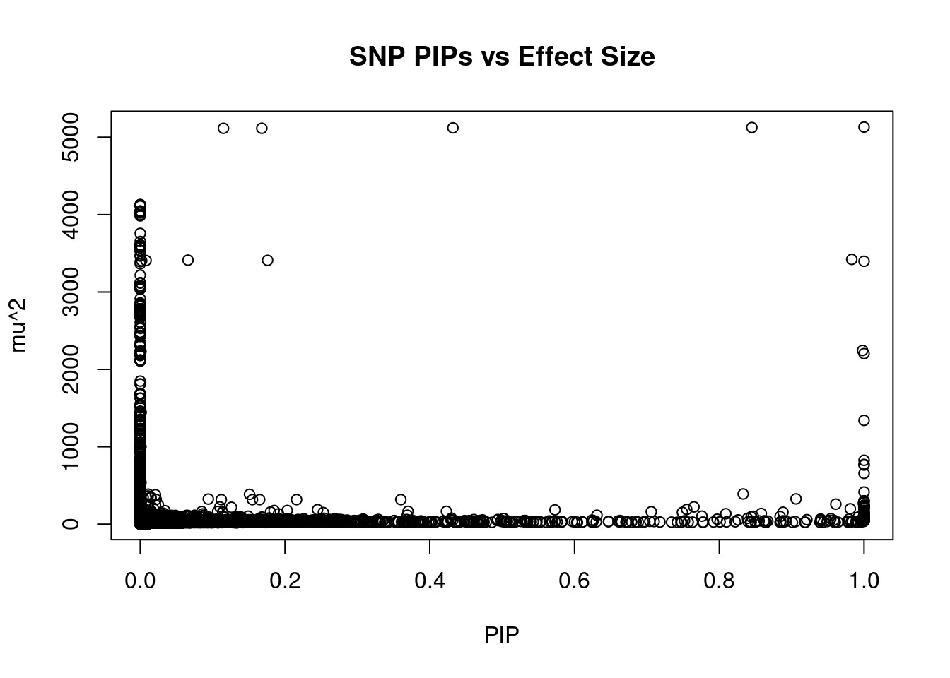
| Version | Author | Date |
|---|---|---|
| dfd2b5f | wesleycrouse | 2021-09-07 |
#SNPs with 50 largest effect sizes
head(ctwas_snp_res[order(-ctwas_snp_res$mu2),report_cols_snps],50)
id region_tag susie_pip mu2 PVE z
909107 rs10677712 2_69 1.000 5131.08 1.5e-02 5.35
909103 rs28850371 2_69 0.845 5125.59 1.3e-02 4.97
909064 rs6542385 2_69 0.432 5120.71 6.4e-03 4.99
909111 rs1546621 2_69 0.168 5115.67 2.5e-03 4.98
909116 rs1516006 2_69 0.115 5115.15 1.7e-03 4.97
909092 rs151256241 2_69 0.000 4130.93 4.5e-16 5.50
909112 rs2551674 2_69 0.000 4126.50 3.9e-16 5.48
909124 rs2245241 2_69 0.000 4124.16 3.7e-16 5.46
909127 rs2674843 2_69 0.000 4122.30 3.6e-16 5.46
909175 rs2255565 2_69 0.000 4110.59 3.5e-16 5.45
909101 rs36144266 2_69 0.000 4047.10 9.1e-14 5.33
909099 rs201120706 2_69 0.000 4046.06 8.8e-14 5.32
909109 rs7575129 2_69 0.000 4042.28 9.4e-14 5.36
909118 rs965193 2_69 0.000 4041.02 6.9e-14 5.30
909055 rs4117160 2_69 0.000 4037.74 8.2e-14 5.34
908973 rs1516009 2_69 0.000 4021.13 1.1e-13 5.39
909053 rs2551687 2_69 0.000 3997.51 2.1e-14 6.04
909047 rs2551685 2_69 0.000 3996.96 2.9e-14 6.10
908983 rs2551684 2_69 0.000 3983.78 3.3e-14 6.12
908991 rs11695801 2_69 0.000 3757.94 3.1e-14 5.24
909201 rs2551679 2_69 0.000 3652.92 2.7e-15 4.86
909144 rs2263642 2_69 0.000 3604.28 1.1e-11 5.73
909134 rs2216845 2_69 0.000 3603.77 9.5e-12 5.72
909182 rs2161843 2_69 0.000 3603.38 9.9e-12 5.73
909156 rs2244678 2_69 0.000 3603.06 9.6e-12 5.72
909183 rs2194495 2_69 0.000 3603.05 9.6e-12 5.72
909172 rs2255586 2_69 0.000 3603.03 9.5e-12 5.72
909173 rs2674847 2_69 0.000 3603.03 9.5e-12 5.72
909165 rs2674849 2_69 0.000 3603.02 9.5e-12 5.72
909169 rs2551677 2_69 0.000 3603.02 9.5e-12 5.72
909171 rs2255590 2_69 0.000 3603.02 9.5e-12 5.72
909161 rs962316 2_69 0.000 3603.01 9.5e-12 5.72
909164 rs962314 2_69 0.000 3603.01 9.5e-12 5.72
909155 rs2244681 2_69 0.000 3602.99 9.5e-12 5.72
909157 rs2244676 2_69 0.000 3602.99 9.5e-12 5.72
909160 rs2911659 2_69 0.000 3602.99 9.5e-12 5.72
909152 rs2421964 2_69 0.000 3602.77 8.2e-12 5.70
909153 rs2421965 2_69 0.000 3602.77 8.3e-12 5.70
909145 rs2674855 2_69 0.000 3602.42 8.9e-12 5.71
909147 rs2674853 2_69 0.000 3602.42 8.9e-12 5.71
909136 rs2161844 2_69 0.000 3602.41 8.9e-12 5.71
909138 rs2674857 2_69 0.000 3602.41 8.9e-12 5.71
909140 rs2263639 2_69 0.000 3602.41 8.9e-12 5.71
909142 rs2263640 2_69 0.000 3602.40 8.9e-12 5.71
909143 rs2263641 2_69 0.000 3602.40 8.9e-12 5.71
909150 rs2421963 2_69 0.000 3602.40 8.9e-12 5.71
909159 rs2244671 2_69 0.000 3601.70 1.0e-11 5.74
909158 rs2244672 2_69 0.000 3601.32 8.1e-12 5.70
909148 rs2263643 2_69 0.000 3600.05 8.2e-12 5.70
909137 rs2674858 2_69 0.000 3592.28 1.2e-11 5.76SNPs with highest PVE
#SNPs with 50 highest pve
head(ctwas_snp_res[order(-ctwas_snp_res$PVE),report_cols_snps],50)
id region_tag susie_pip mu2 PVE z
909107 rs10677712 2_69 1.000 5131.08 0.01500 5.35
909103 rs28850371 2_69 0.845 5125.59 0.01300 4.97
402338 rs763798411 7_65 1.000 3396.95 0.00990 -3.27
402349 rs4997569 7_65 0.983 3421.12 0.00980 -2.98
787130 rs147985405 19_9 0.998 2244.61 0.00650 -48.94
797303 rs814573 19_32 1.000 2204.08 0.00640 55.54
909064 rs6542385 2_69 0.432 5120.71 0.00640 4.99
797308 rs12721109 19_32 1.000 1341.07 0.00390 -46.33
909111 rs1546621 2_69 0.168 5115.67 0.00250 4.98
797252 rs62117204 19_32 1.000 825.46 0.00240 -44.67
797270 rs111794050 19_32 1.000 763.45 0.00220 -33.60
797305 rs113345881 19_32 1.000 772.05 0.00220 -34.32
68016 rs548145 2_13 1.000 656.38 0.00190 33.09
402344 rs13230660 7_65 0.176 3408.94 0.00170 -2.95
909116 rs1516006 2_69 0.115 5115.15 0.00170 4.97
68013 rs934197 2_13 1.000 415.42 0.00120 33.06
279270 rs3843482 5_45 0.833 389.97 0.00095 25.03
500347 rs115478735 9_70 1.000 302.07 0.00088 19.01
159815 rs768688512 3_58 1.000 299.22 0.00087 2.62
14016 rs1887552 1_34 0.906 326.57 0.00086 -9.87
14015 rs2495502 1_34 1.000 283.40 0.00082 6.29
787138 rs1569372 19_9 0.999 268.64 0.00078 10.01
459797 rs79658059 8_83 0.961 258.88 0.00072 -16.02
789919 rs2285626 19_15 1.000 245.82 0.00072 -18.22
1025628 rs964184 11_70 1.000 238.94 0.00070 -16.66
787109 rs73013176 19_9 1.000 237.06 0.00069 -16.23
68007 rs1042034 2_13 1.000 233.16 0.00068 16.57
365688 rs12208357 6_103 1.000 234.69 0.00068 12.28
68093 rs1848922 2_13 1.000 229.86 0.00067 25.41
402341 rs10274607 7_65 0.066 3411.59 0.00065 -2.87
459808 rs13252684 8_83 1.000 216.75 0.00063 11.96
789944 rs3794991 19_15 1.000 212.34 0.00062 -21.49
14033 rs471705 1_34 1.000 207.62 0.00060 16.26
279247 rs10062361 5_45 0.981 198.66 0.00057 20.32
797011 rs62115478 19_30 1.000 180.20 0.00052 -14.33
907894 rs6544713 2_27 0.765 223.21 0.00050 -20.38
69743 rs780093 2_16 1.000 160.70 0.00047 -14.14
365702 rs3818678 6_103 0.755 190.33 0.00042 -9.95
753688 rs113408695 17_39 1.000 143.15 0.00042 12.77
753714 rs8070232 17_39 1.000 144.03 0.00042 -8.09
724532 rs821840 16_31 0.888 154.65 0.00040 -13.48
14026 rs10888896 1_34 1.000 131.45 0.00038 11.89
67958 rs11679386 2_12 1.000 127.41 0.00037 11.91
1058611 rs763665 16_38 0.858 137.84 0.00034 -11.29
159811 rs73141241 3_58 0.360 317.03 0.00033 2.80
304153 rs12657266 5_92 0.749 153.04 0.00033 13.89
787147 rs137992968 19_9 1.000 112.56 0.00033 -10.75
1058618 rs77303550 16_38 0.706 160.91 0.00033 -13.73
753699 rs9303012 17_39 0.809 135.17 0.00032 2.26
440145 rs4738679 8_45 1.000 106.62 0.00031 -11.70SNPs with largest z scores
#SNPs with 50 largest z scores
head(ctwas_snp_res[order(-abs(ctwas_snp_res$z)),report_cols_snps],50)
id region_tag susie_pip mu2 PVE z
797303 rs814573 19_32 1.000 2204.08 6.4e-03 55.54
787130 rs147985405 19_9 0.998 2244.61 6.5e-03 -48.94
787125 rs73015020 19_9 0.001 2232.73 5.8e-06 -48.80
787123 rs138175288 19_9 0.000 2230.92 2.7e-06 -48.78
787124 rs138294113 19_9 0.000 2226.92 6.8e-07 -48.75
787126 rs77140532 19_9 0.000 2227.54 4.1e-07 -48.74
787127 rs112552009 19_9 0.000 2223.23 2.0e-07 -48.71
787128 rs10412048 19_9 0.000 2224.26 8.5e-08 -48.70
787122 rs55997232 19_9 0.000 2203.75 1.1e-10 -48.52
797308 rs12721109 19_32 1.000 1341.07 3.9e-03 -46.33
797252 rs62117204 19_32 1.000 825.46 2.4e-03 -44.67
797239 rs1551891 19_32 0.000 505.03 0.0e+00 -42.27
874870 rs12740374 1_67 0.001 1447.11 2.2e-06 -41.79
874866 rs7528419 1_67 0.001 1443.10 2.2e-06 -41.74
874877 rs646776 1_67 0.000 1441.92 1.9e-06 41.73
874876 rs629301 1_67 0.000 1438.27 1.8e-06 41.69
874888 rs583104 1_67 0.000 1398.08 1.9e-06 41.09
874891 rs4970836 1_67 0.000 1395.22 1.8e-06 41.05
874893 rs1277930 1_67 0.000 1390.56 1.9e-06 40.98
874894 rs599839 1_67 0.000 1389.62 1.9e-06 40.96
787131 rs17248769 19_9 0.000 1690.84 7.6e-09 -40.84
787132 rs2228671 19_9 0.000 1679.78 5.2e-09 -40.70
874874 rs3832016 1_67 0.000 1351.22 1.3e-06 40.40
874871 rs660240 1_67 0.000 1344.09 1.3e-06 40.29
874889 rs602633 1_67 0.000 1323.03 1.4e-06 39.96
787121 rs9305020 19_9 0.000 1277.38 1.7e-16 -34.84
797299 rs405509 19_32 0.000 976.81 0.0e+00 -34.64
874857 rs4970834 1_67 0.001 999.83 2.1e-06 -34.62
797305 rs113345881 19_32 1.000 772.05 2.2e-03 -34.32
797223 rs62120566 19_32 0.000 1321.05 0.0e+00 -33.74
797270 rs111794050 19_32 1.000 763.45 2.2e-03 -33.60
68016 rs548145 2_13 1.000 656.38 1.9e-03 33.09
797276 rs4802238 19_32 0.000 977.73 0.0e+00 33.08
68013 rs934197 2_13 1.000 415.42 1.2e-03 33.06
797217 rs188099946 19_32 0.000 1266.33 0.0e+00 -33.04
797287 rs2972559 19_32 0.000 1298.67 0.0e+00 32.29
797211 rs201314191 19_32 0.000 1174.47 0.0e+00 -32.07
874878 rs3902354 1_67 0.000 853.26 9.4e-07 32.00
874867 rs11102967 1_67 0.000 849.66 9.4e-07 31.94
874892 rs4970837 1_67 0.000 846.20 1.1e-06 31.86
797278 rs56394238 19_32 0.000 968.79 0.0e+00 31.55
797255 rs2965169 19_32 0.000 367.34 0.0e+00 -31.38
797279 rs3021439 19_32 0.000 864.36 0.0e+00 31.05
874862 rs611917 1_67 0.000 800.71 8.4e-07 -30.98
68043 rs12997242 2_13 0.000 384.12 6.4e-14 30.82
797286 rs12162222 19_32 0.000 1112.90 0.0e+00 30.50
68017 rs478588 2_13 0.000 604.36 2.6e-13 30.49
797216 rs62119327 19_32 0.000 1034.69 0.0e+00 -30.42
68018 rs56350433 2_13 0.000 351.24 6.1e-15 30.23
68023 rs56079819 2_13 0.000 350.44 6.1e-15 30.19Gene set enrichment for genes with PIP>0.8
#GO enrichment analysis
library(enrichR)
Welcome to enrichR
Checking connection ... Enrichr ... Connection is Live!
FlyEnrichr ... Connection is available!
WormEnrichr ... Connection is available!
YeastEnrichr ... Connection is available!
FishEnrichr ... Connection is available!dbs <- c("GO_Biological_Process_2021", "GO_Cellular_Component_2021", "GO_Molecular_Function_2021")
genes <- ctwas_gene_res$genename[ctwas_gene_res$susie_pip>0.8]
#number of genes for gene set enrichment
length(genes)[1] 33if (length(genes)>0){
GO_enrichment <- enrichr(genes, dbs)
for (db in dbs){
print(db)
df <- GO_enrichment[[db]]
df <- df[df$Adjusted.P.value<0.05,c("Term", "Overlap", "Adjusted.P.value", "Genes")]
print(df)
}
#DisGeNET enrichment
# devtools::install_bitbucket("ibi_group/disgenet2r")
library(disgenet2r)
disgenet_api_key <- get_disgenet_api_key(
email = "wesleycrouse@gmail.com",
password = "uchicago1" )
Sys.setenv(DISGENET_API_KEY= disgenet_api_key)
res_enrich <-disease_enrichment(entities=genes, vocabulary = "HGNC",
database = "CURATED" )
df <- res_enrich@qresult[1:10, c("Description", "FDR", "Ratio", "BgRatio")]
print(df)
#WebGestalt enrichment
library(WebGestaltR)
background <- ctwas_gene_res$genename
#listGeneSet()
databases <- c("pathway_KEGG", "disease_GLAD4U", "disease_OMIM")
enrichResult <- WebGestaltR(enrichMethod="ORA", organism="hsapiens",
interestGene=genes, referenceGene=background,
enrichDatabase=databases, interestGeneType="genesymbol",
referenceGeneType="genesymbol", isOutput=F)
print(enrichResult[,c("description", "size", "overlap", "FDR", "database", "userId")])
}Uploading data to Enrichr... Done.
Querying GO_Biological_Process_2021... Done.
Querying GO_Cellular_Component_2021... Done.
Querying GO_Molecular_Function_2021... Done.
Parsing results... Done.
[1] "GO_Biological_Process_2021"
Term Overlap
1 peptidyl-serine phosphorylation (GO:0018105) 5/156
2 peptidyl-serine modification (GO:0018209) 5/169
3 lipid transport (GO:0006869) 4/109
4 cholesterol transport (GO:0030301) 3/51
5 intestinal cholesterol absorption (GO:0030299) 2/9
6 cellular response to sterol depletion (GO:0071501) 2/9
7 negative regulation of cholesterol storage (GO:0010887) 2/10
8 protein phosphorylation (GO:0006468) 6/496
9 intestinal lipid absorption (GO:0098856) 2/11
10 cholesterol homeostasis (GO:0042632) 3/71
11 sterol homeostasis (GO:0055092) 3/72
12 cholesterol metabolic process (GO:0008203) 3/77
13 regulation of cholesterol storage (GO:0010885) 2/16
14 activin receptor signaling pathway (GO:0032924) 2/19
15 negative regulation of lipid storage (GO:0010888) 2/20
16 sterol transport (GO:0015918) 2/21
17 cholesterol efflux (GO:0033344) 2/24
18 regulation of DNA biosynthetic process (GO:2000278) 2/29
19 cellular protein modification process (GO:0006464) 7/1025
20 regulation of cholesterol efflux (GO:0010874) 2/33
21 secondary alcohol biosynthetic process (GO:1902653) 2/34
22 organic substance transport (GO:0071702) 3/136
23 cholesterol biosynthetic process (GO:0006695) 2/35
24 sterol biosynthetic process (GO:0016126) 2/38
Adjusted.P.value Genes
1 0.001778112 CSNK1G3;TNKS;PKN3;PRKD2;GAS6
2 0.001778112 CSNK1G3;TNKS;PKN3;PRKD2;GAS6
3 0.004505375 ABCA1;ABCG8;NPC1L1;PLTP
4 0.007029494 ABCA1;ABCG8;NPC1L1
5 0.007029494 ABCG8;NPC1L1
6 0.007029494 INSIG2;NPC1L1
7 0.007144915 ABCA1;TTC39B
8 0.007144915 CSNK1G3;ACVR1C;TNKS;PKN3;PRKD2;GAS6
9 0.007144915 ABCG8;NPC1L1
10 0.009177895 ABCA1;ABCG8;TTC39B
11 0.009177895 ABCA1;ABCG8;TTC39B
12 0.010261090 ABCA1;INSIG2;NPC1L1
13 0.010736790 ABCA1;TTC39B
14 0.014163171 ACVR1C;INHBB
15 0.014672589 ABCA1;TTC39B
16 0.015187830 ABCG8;NPC1L1
17 0.018728919 ABCA1;ABCG8
18 0.025886117 TNKS;PRKD2
19 0.028304765 CSNK1G3;ACVR1C;TNKS;PKN3;PRKD2;FUT2;GAS6
20 0.029365079 PLTP;TTC39B
21 0.029365079 INSIG2;NPC1L1
22 0.029365079 ABCA1;ABCG8;PLTP
23 0.029506425 INSIG2;NPC1L1
24 0.033306505 INSIG2;NPC1L1
[1] "GO_Cellular_Component_2021"
Term Overlap Adjusted.P.value
1 high-density lipoprotein particle (GO:0034364) 2/19 0.01641280
2 endoplasmic reticulum membrane (GO:0005789) 6/712 0.01794926
Genes
1 HPR;PLTP
2 ABCA1;CYP2A6;INSIG2;KDSR;FADS1;CNIH4
[1] "GO_Molecular_Function_2021"
Term Overlap
1 cholesterol transfer activity (GO:0120020) 3/18
2 sterol transfer activity (GO:0120015) 3/19
3 phosphatidylcholine transporter activity (GO:0008525) 2/18
Adjusted.P.value Genes
1 0.0001655238 ABCA1;ABCG8;PLTP
2 0.0001655238 ABCA1;ABCG8;PLTP
3 0.0112569839 ABCA1;PLTPPELO gene(s) from the input list not found in DisGeNET CURATEDSPTY2D1 gene(s) from the input list not found in DisGeNET CURATEDRP4-781K5.7 gene(s) from the input list not found in DisGeNET CURATEDC10orf88 gene(s) from the input list not found in DisGeNET CURATEDTRIM39 gene(s) from the input list not found in DisGeNET CURATEDACP6 gene(s) from the input list not found in DisGeNET CURATEDDDX56 gene(s) from the input list not found in DisGeNET CURATEDCRACR2B gene(s) from the input list not found in DisGeNET CURATEDTTC39B gene(s) from the input list not found in DisGeNET CURATEDPSRC1 gene(s) from the input list not found in DisGeNET CURATEDCSNK1G3 gene(s) from the input list not found in DisGeNET CURATEDUSP1 gene(s) from the input list not found in DisGeNET CURATEDTNKS gene(s) from the input list not found in DisGeNET CURATEDHPR gene(s) from the input list not found in DisGeNET CURATEDPOP7 gene(s) from the input list not found in DisGeNET CURATEDPKN3 gene(s) from the input list not found in DisGeNET CURATEDNPC1L1 gene(s) from the input list not found in DisGeNET CURATEDCNIH4 gene(s) from the input list not found in DisGeNET CURATED Description FDR Ratio BgRatio
5 Blood Platelet Disorders 0.01214043 2/15 16/9703
21 Hypercholesterolemia 0.01214043 2/15 39/9703
22 Hypercholesterolemia, Familial 0.01214043 2/15 18/9703
36 Opisthorchiasis 0.01214043 1/15 1/9703
43 Tangier Disease 0.01214043 1/15 1/9703
57 Caliciviridae Infections 0.01214043 1/15 1/9703
63 Infections, Calicivirus 0.01214043 1/15 1/9703
77 Opisthorchis felineus Infection 0.01214043 1/15 1/9703
78 Opisthorchis viverrini Infection 0.01214043 1/15 1/9703
89 Hypoalphalipoproteinemias 0.01214043 1/15 1/9703******************************************
* *
* Welcome to WebGestaltR ! *
* *
******************************************Loading the functional categories...
Loading the ID list...
Loading the reference list...
Performing the enrichment analysis...
description size overlap FDR database
1 Coronary Artery Disease 153 10 1.274177e-07 disease_GLAD4U
2 Dyslipidaemia 84 8 3.535758e-07 disease_GLAD4U
3 Coronary Disease 171 9 3.202353e-06 disease_GLAD4U
4 Arteriosclerosis 173 8 5.579161e-05 disease_GLAD4U
5 Myocardial Ischemia 181 8 6.337034e-05 disease_GLAD4U
6 Arterial Occlusive Diseases 174 7 5.907884e-04 disease_GLAD4U
7 Hypercholesterolemia 60 5 5.907884e-04 disease_GLAD4U
8 Heart Diseases 227 7 2.988516e-03 disease_GLAD4U
9 Cardiovascular Diseases 282 7 1.082847e-02 disease_GLAD4U
10 Fat digestion and absorption 23 3 1.407039e-02 pathway_KEGG
11 Hyperlipidemias 64 4 1.407039e-02 disease_GLAD4U
12 Vascular Diseases 234 6 2.609523e-02 disease_GLAD4U
13 Cholesterol metabolism 31 3 2.854433e-02 pathway_KEGG
14 Obesity 172 5 4.854820e-02 disease_GLAD4U
userId
1 PSRC1;ABCG8;INSIG2;NPC1L1;TTC39B;ABCA1;SPTY2D1;FADS1;FUT2;PLTP
2 PSRC1;ABCG8;INSIG2;NPC1L1;TTC39B;ABCA1;FADS1;PLTP
3 PSRC1;ABCG8;INSIG2;NPC1L1;TTC39B;ABCA1;FADS1;FUT2;PLTP
4 PSRC1;ABCG8;NPC1L1;TTC39B;ABCA1;FADS1;HPR;PLTP
5 PSRC1;ABCG8;INSIG2;NPC1L1;TTC39B;ABCA1;FADS1;PLTP
6 PSRC1;ABCG8;NPC1L1;TTC39B;ABCA1;FADS1;PLTP
7 ABCG8;INSIG2;NPC1L1;ABCA1;PLTP
8 PSRC1;ABCG8;NPC1L1;TTC39B;ABCA1;FADS1;PLTP
9 PSRC1;ABCG8;TTC39B;ABCA1;FADS1;GAS6;PLTP
10 ABCG8;NPC1L1;ABCA1
11 ABCG8;NPC1L1;ABCA1;PLTP
12 PSRC1;ABCG8;NPC1L1;ABCA1;GAS6;PLTP
13 ABCG8;ABCA1;PLTP
14 INSIG2;TTC39B;ABCA1;FADS1;PLTP
sessionInfo()R version 3.6.1 (2019-07-05)
Platform: x86_64-pc-linux-gnu (64-bit)
Running under: Scientific Linux 7.4 (Nitrogen)
Matrix products: default
BLAS/LAPACK: /software/openblas-0.2.19-el7-x86_64/lib/libopenblas_haswellp-r0.2.19.so
locale:
[1] LC_CTYPE=en_US.UTF-8 LC_NUMERIC=C
[3] LC_TIME=en_US.UTF-8 LC_COLLATE=en_US.UTF-8
[5] LC_MONETARY=en_US.UTF-8 LC_MESSAGES=en_US.UTF-8
[7] LC_PAPER=en_US.UTF-8 LC_NAME=C
[9] LC_ADDRESS=C LC_TELEPHONE=C
[11] LC_MEASUREMENT=en_US.UTF-8 LC_IDENTIFICATION=C
attached base packages:
[1] stats graphics grDevices utils datasets methods base
other attached packages:
[1] WebGestaltR_0.4.4 disgenet2r_0.99.2 enrichR_3.0 cowplot_1.0.0
[5] ggplot2_3.3.3
loaded via a namespace (and not attached):
[1] bitops_1.0-6 matrixStats_0.57.0
[3] fs_1.3.1 bit64_4.0.5
[5] doParallel_1.0.16 progress_1.2.2
[7] httr_1.4.1 rprojroot_2.0.2
[9] GenomeInfoDb_1.20.0 doRNG_1.8.2
[11] tools_3.6.1 utf8_1.2.1
[13] R6_2.5.0 DBI_1.1.1
[15] BiocGenerics_0.30.0 colorspace_1.4-1
[17] withr_2.4.1 tidyselect_1.1.0
[19] prettyunits_1.0.2 bit_4.0.4
[21] curl_3.3 compiler_3.6.1
[23] git2r_0.26.1 Biobase_2.44.0
[25] DelayedArray_0.10.0 rtracklayer_1.44.0
[27] labeling_0.3 scales_1.1.0
[29] readr_1.4.0 apcluster_1.4.8
[31] stringr_1.4.0 digest_0.6.20
[33] Rsamtools_2.0.0 svglite_1.2.2
[35] rmarkdown_1.13 XVector_0.24.0
[37] pkgconfig_2.0.3 htmltools_0.3.6
[39] fastmap_1.1.0 BSgenome_1.52.0
[41] rlang_0.4.11 RSQLite_2.2.7
[43] generics_0.0.2 farver_2.1.0
[45] jsonlite_1.6 BiocParallel_1.18.0
[47] dplyr_1.0.7 VariantAnnotation_1.30.1
[49] RCurl_1.98-1.1 magrittr_2.0.1
[51] GenomeInfoDbData_1.2.1 Matrix_1.2-18
[53] Rcpp_1.0.6 munsell_0.5.0
[55] S4Vectors_0.22.1 fansi_0.5.0
[57] gdtools_0.1.9 lifecycle_1.0.0
[59] stringi_1.4.3 whisker_0.3-2
[61] yaml_2.2.0 SummarizedExperiment_1.14.1
[63] zlibbioc_1.30.0 plyr_1.8.4
[65] grid_3.6.1 blob_1.2.1
[67] parallel_3.6.1 promises_1.0.1
[69] crayon_1.4.1 lattice_0.20-38
[71] Biostrings_2.52.0 GenomicFeatures_1.36.3
[73] hms_1.1.0 knitr_1.23
[75] pillar_1.6.1 igraph_1.2.4.1
[77] GenomicRanges_1.36.0 rjson_0.2.20
[79] rngtools_1.5 codetools_0.2-16
[81] reshape2_1.4.3 biomaRt_2.40.1
[83] stats4_3.6.1 XML_3.98-1.20
[85] glue_1.4.2 evaluate_0.14
[87] data.table_1.14.0 foreach_1.5.1
[89] vctrs_0.3.8 httpuv_1.5.1
[91] gtable_0.3.0 purrr_0.3.4
[93] assertthat_0.2.1 cachem_1.0.5
[95] xfun_0.8 later_0.8.0
[97] tibble_3.1.2 iterators_1.0.13
[99] GenomicAlignments_1.20.1 AnnotationDbi_1.46.0
[101] memoise_2.0.0 IRanges_2.18.1
[103] workflowr_1.6.2 ellipsis_0.3.2