Glucose - Pancreas
wesleycrouse
2021-09-7
Last updated: 2021-09-13
Checks: 7 0
Knit directory: ctwas_applied/
This reproducible R Markdown analysis was created with workflowr (version 1.6.2). The Checks tab describes the reproducibility checks that were applied when the results were created. The Past versions tab lists the development history.
Great! Since the R Markdown file has been committed to the Git repository, you know the exact version of the code that produced these results.
Great job! The global environment was empty. Objects defined in the global environment can affect the analysis in your R Markdown file in unknown ways. For reproduciblity it’s best to always run the code in an empty environment.
The command set.seed(20210726) was run prior to running the code in the R Markdown file. Setting a seed ensures that any results that rely on randomness, e.g. subsampling or permutations, are reproducible.
Great job! Recording the operating system, R version, and package versions is critical for reproducibility.
Nice! There were no cached chunks for this analysis, so you can be confident that you successfully produced the results during this run.
Great job! Using relative paths to the files within your workflowr project makes it easier to run your code on other machines.
Great! You are using Git for version control. Tracking code development and connecting the code version to the results is critical for reproducibility.
The results in this page were generated with repository version 72c8ef7. See the Past versions tab to see a history of the changes made to the R Markdown and HTML files.
Note that you need to be careful to ensure that all relevant files for the analysis have been committed to Git prior to generating the results (you can use wflow_publish or wflow_git_commit). workflowr only checks the R Markdown file, but you know if there are other scripts or data files that it depends on. Below is the status of the Git repository when the results were generated:
working directory clean
Note that any generated files, e.g. HTML, png, CSS, etc., are not included in this status report because it is ok for generated content to have uncommitted changes.
These are the previous versions of the repository in which changes were made to the R Markdown (analysis/ukb-d-30740_irnt_Pancreas_known.Rmd) and HTML (docs/ukb-d-30740_irnt_Pancreas_known.html) files. If you’ve configured a remote Git repository (see ?wflow_git_remote), click on the hyperlinks in the table below to view the files as they were in that past version.
| File | Version | Author | Date | Message |
|---|---|---|---|---|
| Rmd | 72c8ef7 | wesleycrouse | 2021-09-13 | changing mart for biomart |
| Rmd | a49c40e | wesleycrouse | 2021-09-13 | updating with bystander analysis |
| html | 7e22565 | wesleycrouse | 2021-09-13 | updating reports |
| html | 0c9ef1c | wesleycrouse | 2021-09-08 | adding first two reports |
| Rmd | cbf7408 | wesleycrouse | 2021-09-08 | adding enrichment to reports |
Overview
These are the results of a ctwas analysis of the UK Biobank trait Glucose using Pancreas gene weights.
The GWAS was conducted by the Neale Lab, and the biomarker traits we analyzed are discussed here. Summary statistics were obtained from IEU OpenGWAS using GWAS ID: ukb-d-30740_irnt. Results were obtained from from IEU rather than Neale Lab because they are in a standardard format (GWAS VCF). Note that 3 of the 34 biomarker traits were not available from IEU and were excluded from analysis.
The weights are mashr GTEx v8 models on Pancreas eQTL obtained from PredictDB. We performed a full harmonization of the variants, including recovering strand ambiguous variants. This procedure is discussed in a separate document. (TO-DO: add report that describes harmonization)
LD matrices were computed from a 10% subset of Neale lab subjects. Subjects were matched using the plate and well information from genotyping. We included only biallelic variants with MAF>0.01 in the original Neale Lab GWAS. (TO-DO: add more details [number of subjects, variants, etc])
Weight QC
TO-DO: add enhanced QC reporting (total number of weights, why each variant was missing for all genes)
qclist_all <- list()

qc_files <- paste0(results_dir, "/", list.files(results_dir, pattern="exprqc.Rd"))

for (i in 1:length(qc_files)){
  load(qc_files[i])
  chr <- unlist(strsplit(rev(unlist(strsplit(qc_files[i], "_")))[1], "[.]"))[1]
  qclist_all[[chr]] <- cbind(do.call(rbind, lapply(qclist,unlist)), as.numeric(substring(chr,4)))
}

qclist_all <- data.frame(do.call(rbind, qclist_all))
colnames(qclist_all)[ncol(qclist_all)] <- "chr"

rm(qclist, wgtlist, z_gene_chr)

#number of imputed weights
nrow(qclist_all)
[1] 11855#number of imputed weights by chromosome
table(qclist_all$chr)
   1    2    3    4    5    6    7    8    9   10   11   12   13   14   15
1153  845  676  460  544  661  589  418  452  468  737  686  225  381  411
  16   17   18   19   20   21   22
 551  734  171  912  359  121  301
#proportion of imputed weights without missing variants
mean(qclist_all$nmiss==0)[1] 0.7999156Load ctwas results
#load ctwas results
ctwas_res <- data.table::fread(paste0(results_dir, "/", analysis_id, "_ctwas.susieIrss.txt"))

#make unique identifier for regions
ctwas_res$region_tag <- paste(ctwas_res$region_tag1, ctwas_res$region_tag2, sep="_")

#load z scores for SNPs and collect sample size
load(paste0(results_dir, "/", analysis_id, "_expr_z_snp.Rd"))

sample_size <- z_snp$ss
sample_size <- as.numeric(names(which.max(table(sample_size))))

#compute PVE for each gene/SNP
ctwas_res$PVE = ctwas_res$susie_pip*ctwas_res$mu2/sample_size

#separate gene and SNP results
ctwas_gene_res <- ctwas_res[ctwas_res$type == "gene", ]
ctwas_gene_res <- data.frame(ctwas_gene_res)
ctwas_snp_res <- ctwas_res[ctwas_res$type == "SNP", ]
ctwas_snp_res <- data.frame(ctwas_snp_res)

#add gene information to results
sqlite <- RSQLite::dbDriver("SQLite")
db = RSQLite::dbConnect(sqlite, paste0("/project2/compbio/predictdb/mashr_models/mashr_", weight, ".db"))
query <- function(...) RSQLite::dbGetQuery(db, ...)
gene_info <- query("select gene, genename from extra")
gene_info <- query("select gene, genename, gene_type from extra")
RSQLite::dbDisconnect(db)

ctwas_gene_res <- cbind(ctwas_gene_res, gene_info[sapply(ctwas_gene_res$id, match, gene_info$gene), c("genename", "gene_type")])

#add z scores to results
load(paste0(results_dir, "/", analysis_id, "_expr_z_gene.Rd"))
ctwas_gene_res$z <- z_gene[ctwas_gene_res$id,]$z

z_snp <- z_snp[z_snp$id %in% ctwas_snp_res$id,]
ctwas_snp_res$z <- z_snp$z[match(ctwas_snp_res$id, z_snp$id)]

#formatting and rounding for tables
ctwas_gene_res$z <- round(ctwas_gene_res$z,2)
ctwas_snp_res$z <- round(ctwas_snp_res$z,2)
ctwas_gene_res$susie_pip <- round(ctwas_gene_res$susie_pip,3)
ctwas_snp_res$susie_pip <- round(ctwas_snp_res$susie_pip,3)
ctwas_gene_res$mu2 <- round(ctwas_gene_res$mu2,2)
ctwas_snp_res$mu2 <- round(ctwas_snp_res$mu2,2)
ctwas_gene_res$PVE <- signif(ctwas_gene_res$PVE, 2)
ctwas_snp_res$PVE <- signif(ctwas_snp_res$PVE, 2)

#merge gene and snp results with added information
ctwas_snp_res$genename=NA
ctwas_snp_res$gene_type=NA

ctwas_res <- rbind(ctwas_gene_res,
                   ctwas_snp_res[,colnames(ctwas_gene_res)])

#store columns to report
report_cols <- colnames(ctwas_gene_res)[!(colnames(ctwas_gene_res) %in% c("type", "region_tag1", "region_tag2", "cs_index", "gene_type", "z_flag", "id", "chrom", "pos"))]
first_cols <- c("genename", "region_tag")
report_cols <- c(first_cols, report_cols[!(report_cols %in% first_cols)])

report_cols_snps <- c("id", report_cols[-1])

#get number of SNPs from s1 results; adjust for thin
ctwas_res_s1 <- data.table::fread(paste0(results_dir, "/", analysis_id, "_ctwas.s1.susieIrss.txt"))
n_snps <- sum(ctwas_res_s1$type=="SNP")/thin
rm(ctwas_res_s1)
Check convergence of parameters
library(ggplot2)
library(cowplot)
********************************************************Note: As of version 1.0.0, cowplot does not change the default ggplot2 theme anymore. To recover the previous behavior, execute:
theme_set(theme_cowplot())********************************************************load(paste0(results_dir, "/", analysis_id, "_ctwas.s2.susieIrssres.Rd"))
df <- data.frame(niter = rep(1:ncol(group_prior_rec), 2),
value = c(group_prior_rec[1,], group_prior_rec[2,]),
group = rep(c("Gene", "SNP"), each = ncol(group_prior_rec)))
df$group <- as.factor(df$group)
df$value[df$group=="SNP"] <- df$value[df$group=="SNP"]*thin #adjust parameter to account for thin argument
p_pi <- ggplot(df, aes(x=niter, y=value, group=group)) +
geom_line(aes(color=group)) +
geom_point(aes(color=group)) +
xlab("Iteration") + ylab(bquote(pi)) +
ggtitle("Prior mean") +
theme_cowplot()
df <- data.frame(niter = rep(1:ncol(group_prior_var_rec), 2),
value = c(group_prior_var_rec[1,], group_prior_var_rec[2,]),
group = rep(c("Gene", "SNP"), each = ncol(group_prior_var_rec)))
df$group <- as.factor(df$group)
p_sigma2 <- ggplot(df, aes(x=niter, y=value, group=group)) +
geom_line(aes(color=group)) +
geom_point(aes(color=group)) +
xlab("Iteration") + ylab(bquote(sigma^2)) +
ggtitle("Prior variance") +
theme_cowplot()
plot_grid(p_pi, p_sigma2)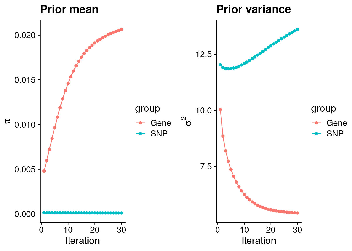
| Version | Author | Date |
|---|---|---|
| 0c9ef1c | wesleycrouse | 2021-09-08 |
#estimated group prior
estimated_group_prior <- group_prior_rec[,ncol(group_prior_rec)]
names(estimated_group_prior) <- c("gene", "snp")
estimated_group_prior["snp"] <- estimated_group_prior["snp"]*thin #adjust parameter to account for thin argument
print(estimated_group_prior)
gene snp
0.0206363187 0.0001156436 #estimated group prior variance
estimated_group_prior_var <- group_prior_var_rec[,ncol(group_prior_var_rec)]
names(estimated_group_prior_var) <- c("gene", "snp")
print(estimated_group_prior_var) gene snp
5.425788 13.611713 #report sample size
print(sample_size)[1] 314916#report group size
group_size <- c(nrow(ctwas_gene_res), n_snps)
print(group_size)[1] 11855 8696600#estimated group PVE
estimated_group_pve <- estimated_group_prior_var*estimated_group_prior*group_size/sample_size #check PVE calculation
names(estimated_group_pve) <- c("gene", "snp")
print(estimated_group_pve) gene snp
0.004215041 0.043469952 #compare sum(PIP*mu2/sample_size) with above PVE calculation
c(sum(ctwas_gene_res$PVE),sum(ctwas_snp_res$PVE))[1] 0.03346152 0.24849702Genes with highest PIPs
#distribution of PIPs
hist(ctwas_gene_res$susie_pip, xlim=c(0,1), main="Distribution of Gene PIPs")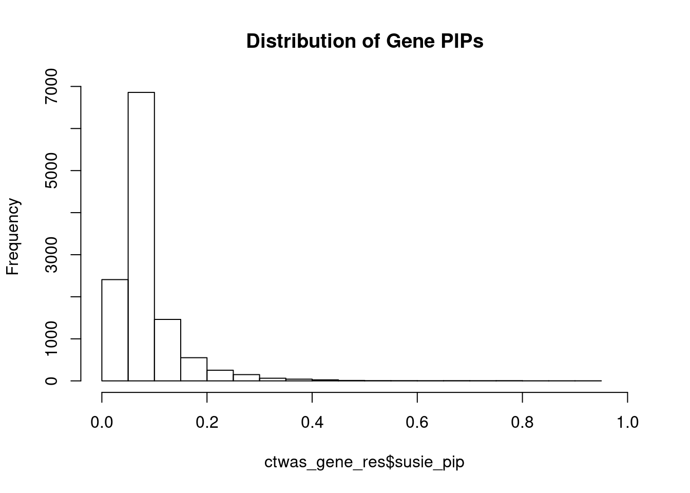
| Version | Author | Date |
|---|---|---|
| 0c9ef1c | wesleycrouse | 2021-09-08 |
#genes with PIP>0.8 or 20 highest PIPs
head(ctwas_gene_res[order(-ctwas_gene_res$susie_pip),report_cols], max(sum(ctwas_gene_res$susie_pip>0.8), 20))
genename region_tag susie_pip mu2 PVE z
13108 SMIM22 16_4 0.913 18.54 5.4e-05 4.21
2726 PTGES3 12_35 0.909 18.45 5.3e-05 4.17
3493 CTNNAL1 9_55 0.878 33.21 9.3e-05 -6.10
342 IKZF2 2_126 0.864 21.03 5.8e-05 4.67
10780 C15orf52 15_14 0.848 21.20 5.7e-05 -4.58
1451 CWF19L1 10_64 0.832 18.41 4.9e-05 -4.12
9996 TMEM45A 3_63 0.794 28.22 7.1e-05 5.77
1480 SIRT1 10_44 0.772 27.03 6.6e-05 5.61
7230 ACE 17_37 0.769 19.95 4.9e-05 4.42
3874 SLC12A5 20_28 0.766 20.75 5.0e-05 -4.10
8621 CTRB2 16_40 0.754 18.40 4.4e-05 4.13
10731 AGRN 1_1 0.744 19.44 4.6e-05 3.85
10565 FAM228A 2_14 0.733 18.87 4.4e-05 -3.94
1794 EEF1A2 20_38 0.714 22.61 5.1e-05 -4.89
2263 CFAP69 7_55 0.704 23.61 5.3e-05 -5.25
5331 THUMPD2 2_25 0.684 18.82 4.1e-05 -3.90
8955 LURAP1 1_28 0.672 20.14 4.3e-05 3.66
8999 LKAAEAR1 20_38 0.671 19.58 4.2e-05 -4.15
3953 RREB1 6_7 0.667 50.00 1.1e-04 6.80
6822 DNAAF1 16_48 0.651 19.39 4.0e-05 -4.07Genes with largest effect sizes
#plot PIP vs effect size
plot(ctwas_gene_res$susie_pip, ctwas_gene_res$mu2, xlab="PIP", ylab="mu^2", main="Gene PIPs vs Effect Size")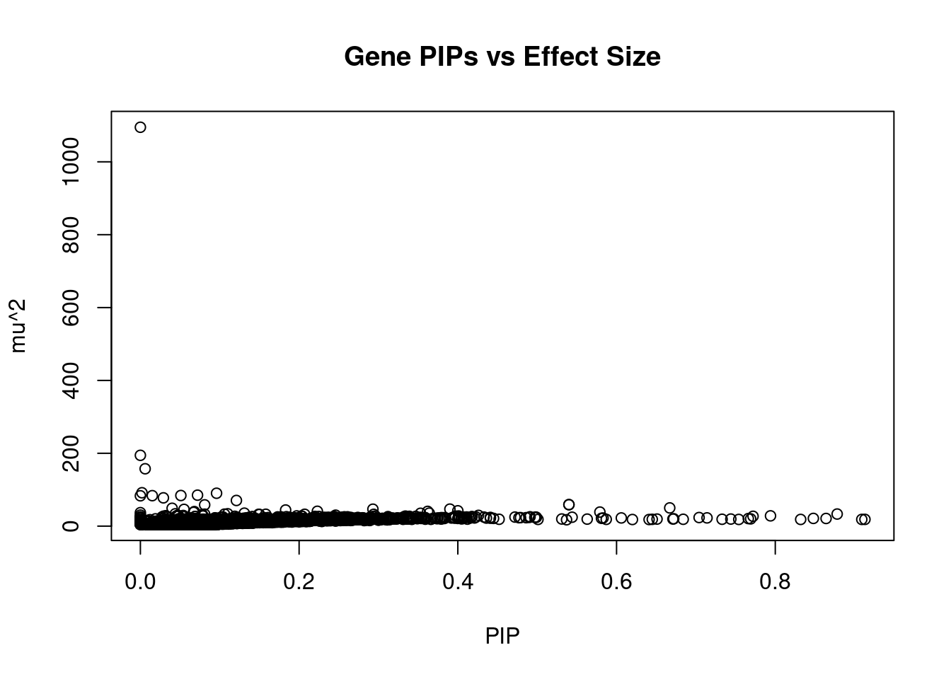
| Version | Author | Date |
|---|---|---|
| 0c9ef1c | wesleycrouse | 2021-09-08 |
#genes with 20 largest effect sizes
head(ctwas_gene_res[order(-ctwas_gene_res$mu2),report_cols],20)
genename region_tag susie_pip mu2 PVE z
6679 G6PC2 2_102 0.000 1094.97 2.7e-12 -37.05
7603 NOSTRIN 2_102 0.000 194.38 7.9e-13 12.79
13656 LINC00506 3_57 0.006 157.46 3.0e-06 -1.94
2366 YKT6 7_32 0.002 91.62 4.9e-07 11.82
3128 NRBP1 2_16 0.096 90.27 2.8e-05 -10.47
3134 PPM1G 2_16 0.072 85.02 1.9e-05 -10.23
487 FOXN3 14_45 0.051 84.06 1.4e-05 10.50
4348 INS-IGF2 11_2 0.015 83.64 3.9e-06 8.52
6678 SPC25 2_102 0.000 83.27 1.3e-11 5.41
7690 SLC2A2 3_104 0.029 77.64 7.0e-06 14.53
13639 LINC01126 2_27 0.121 70.48 2.7e-05 -9.57
11982 AC012354.6 2_28 0.540 58.96 1.0e-04 -8.52
12277 SIX3-AS1 2_28 0.540 58.96 1.0e-04 -8.52
12855 LINC00261 20_16 0.081 58.37 1.5e-05 8.50
3953 RREB1 6_7 0.667 50.00 1.1e-04 6.80
4036 FOXA2 20_16 0.040 49.02 6.3e-06 -7.98
684 SPI1 11_29 0.390 46.72 5.8e-05 8.09
9232 PEAK1 15_36 0.293 46.51 4.3e-05 7.25
12801 RP11-944C7.1 14_45 0.055 46.00 8.1e-06 7.47
6471 FADS1 11_34 0.183 44.24 2.6e-05 7.17Genes with highest PVE
#genes with 20 highest pve
head(ctwas_gene_res[order(-ctwas_gene_res$PVE),report_cols],20)
genename region_tag susie_pip mu2 PVE z
3953 RREB1 6_7 0.667 50.00 1.1e-04 6.80
11982 AC012354.6 2_28 0.540 58.96 1.0e-04 -8.52
12277 SIX3-AS1 2_28 0.540 58.96 1.0e-04 -8.52
3493 CTNNAL1 9_55 0.878 33.21 9.3e-05 -6.10
8288 YWHAB 20_28 0.579 38.59 7.1e-05 6.78
9996 TMEM45A 3_63 0.794 28.22 7.1e-05 5.77
1480 SIRT1 10_44 0.772 27.03 6.6e-05 5.61
684 SPI1 11_29 0.390 46.72 5.8e-05 8.09
342 IKZF2 2_126 0.864 21.03 5.8e-05 4.67
10780 C15orf52 15_14 0.848 21.20 5.7e-05 -4.58
13108 SMIM22 16_4 0.913 18.54 5.4e-05 4.21
2263 CFAP69 7_55 0.704 23.61 5.3e-05 -5.25
11300 C2CD4A 15_29 0.400 42.06 5.3e-05 6.90
2726 PTGES3 12_35 0.909 18.45 5.3e-05 4.17
1794 EEF1A2 20_38 0.714 22.61 5.1e-05 -4.89
3874 SLC12A5 20_28 0.766 20.75 5.0e-05 -4.10
7230 ACE 17_37 0.769 19.95 4.9e-05 4.42
1451 CWF19L1 10_64 0.832 18.41 4.9e-05 -4.12
5132 GAD2 10_19 0.362 40.50 4.7e-05 -6.75
10731 AGRN 1_1 0.744 19.44 4.6e-05 3.85Genes with largest z scores
#genes with 20 largest z scores
head(ctwas_gene_res[order(-abs(ctwas_gene_res$z)),report_cols],20)
genename region_tag susie_pip mu2 PVE z
6679 G6PC2 2_102 0.000 1094.97 2.7e-12 -37.05
7690 SLC2A2 3_104 0.029 77.64 7.0e-06 14.53
7603 NOSTRIN 2_102 0.000 194.38 7.9e-13 12.79
2366 YKT6 7_32 0.002 91.62 4.9e-07 11.82
487 FOXN3 14_45 0.051 84.06 1.4e-05 10.50
3128 NRBP1 2_16 0.096 90.27 2.8e-05 -10.47
3134 PPM1G 2_16 0.072 85.02 1.9e-05 -10.23
13639 LINC01126 2_27 0.121 70.48 2.7e-05 -9.57
11982 AC012354.6 2_28 0.540 58.96 1.0e-04 -8.52
12277 SIX3-AS1 2_28 0.540 58.96 1.0e-04 -8.52
4348 INS-IGF2 11_2 0.015 83.64 3.9e-06 8.52
12855 LINC00261 20_16 0.081 58.37 1.5e-05 8.50
684 SPI1 11_29 0.390 46.72 5.8e-05 8.09
4036 FOXA2 20_16 0.040 49.02 6.3e-06 -7.98
12801 RP11-944C7.1 14_45 0.055 46.00 8.1e-06 7.47
4844 ACP2 11_29 0.048 28.26 4.3e-06 -7.38
9232 PEAK1 15_36 0.293 46.51 4.3e-05 7.25
6471 FADS1 11_34 0.183 44.24 2.6e-05 7.17
132 LUC7L 16_1 0.223 40.80 2.9e-05 7.14
3830 KBTBD4 11_29 0.054 29.20 5.0e-06 -7.05Comparing z scores and PIPs
#set nominal signifiance threshold for z scores
alpha <- 0.05

#bonferroni adjusted threshold for z scores
sig_thresh <- qnorm(1-(alpha/nrow(ctwas_gene_res)/2), lower=T)

#Q-Q plot for z scores
obs_z <- ctwas_gene_res$z[order(ctwas_gene_res$z)]
exp_z <- qnorm((1:nrow(ctwas_gene_res))/nrow(ctwas_gene_res))

plot(exp_z, obs_z, xlab="Expected z", ylab="Observed z", main="Gene z score Q-Q plot")
abline(a=0,b=1)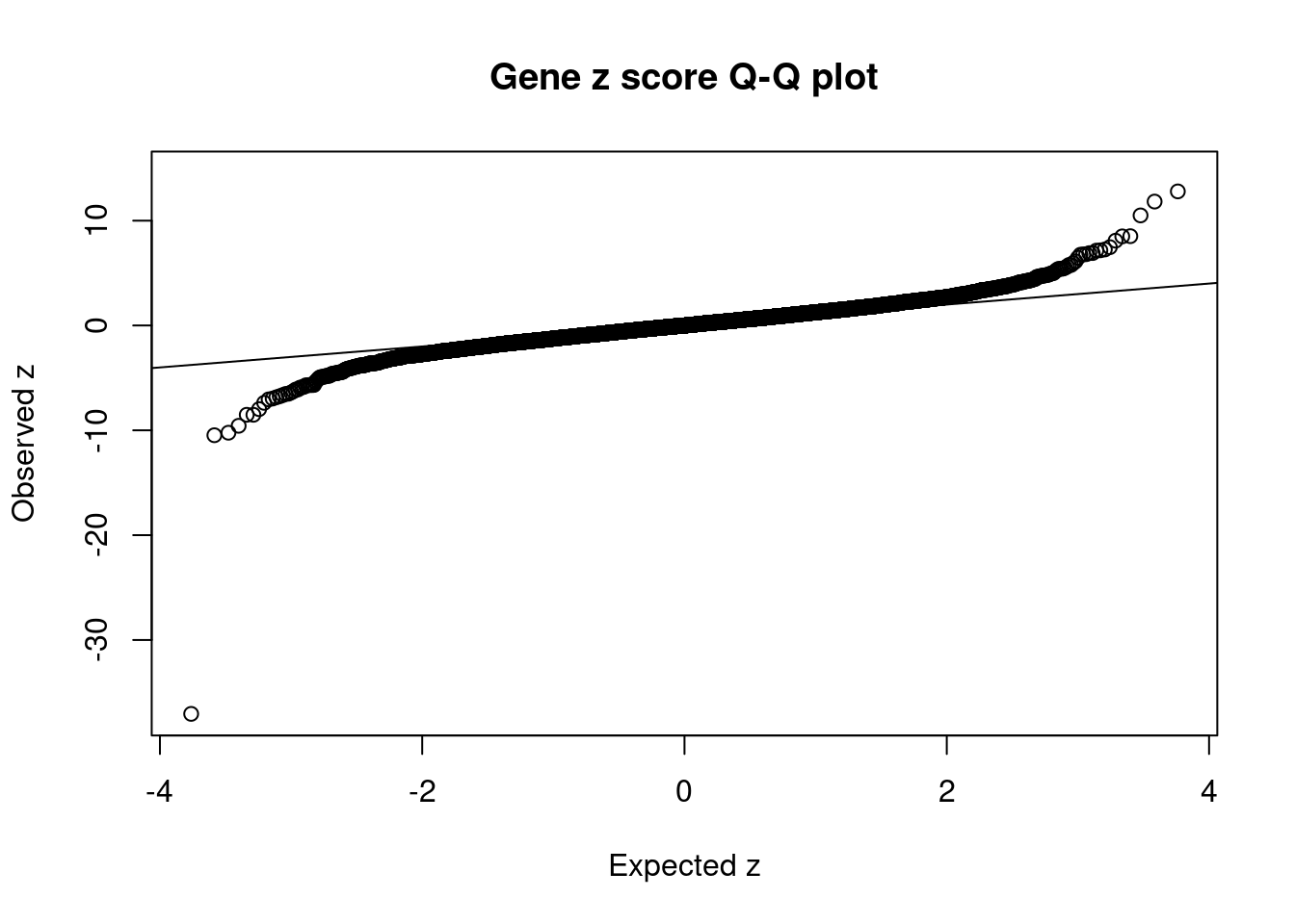
| Version | Author | Date |
|---|---|---|
| 0c9ef1c | wesleycrouse | 2021-09-08 |
#plot z score vs PIP
plot(abs(ctwas_gene_res$z), ctwas_gene_res$susie_pip, xlab="abs(z)", ylab="PIP")
abline(v=sig_thresh, col="red", lty=2)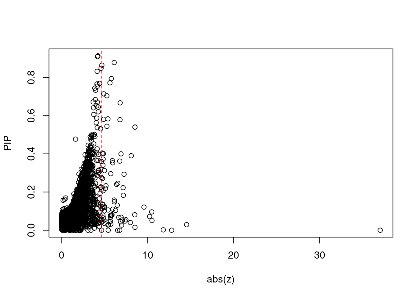
| Version | Author | Date |
|---|---|---|
| 0c9ef1c | wesleycrouse | 2021-09-08 |
#proportion of significant z scores
mean(abs(ctwas_gene_res$z) > sig_thresh)
[1] 0.007338676#genes with most significant z scores
head(ctwas_gene_res[order(-abs(ctwas_gene_res$z)),report_cols],20) genename region_tag susie_pip mu2 PVE z
6679 G6PC2 2_102 0.000 1094.97 2.7e-12 -37.05
7690 SLC2A2 3_104 0.029 77.64 7.0e-06 14.53
7603 NOSTRIN 2_102 0.000 194.38 7.9e-13 12.79
2366 YKT6 7_32 0.002 91.62 4.9e-07 11.82
487 FOXN3 14_45 0.051 84.06 1.4e-05 10.50
3128 NRBP1 2_16 0.096 90.27 2.8e-05 -10.47
3134 PPM1G 2_16 0.072 85.02 1.9e-05 -10.23
13639 LINC01126 2_27 0.121 70.48 2.7e-05 -9.57
11982 AC012354.6 2_28 0.540 58.96 1.0e-04 -8.52
12277 SIX3-AS1 2_28 0.540 58.96 1.0e-04 -8.52
4348 INS-IGF2 11_2 0.015 83.64 3.9e-06 8.52
12855 LINC00261 20_16 0.081 58.37 1.5e-05 8.50
684 SPI1 11_29 0.390 46.72 5.8e-05 8.09
4036 FOXA2 20_16 0.040 49.02 6.3e-06 -7.98
12801 RP11-944C7.1 14_45 0.055 46.00 8.1e-06 7.47
4844 ACP2 11_29 0.048 28.26 4.3e-06 -7.38
9232 PEAK1 15_36 0.293 46.51 4.3e-05 7.25
6471 FADS1 11_34 0.183 44.24 2.6e-05 7.17
132 LUC7L 16_1 0.223 40.80 2.9e-05 7.14
3830 KBTBD4 11_29 0.054 29.20 5.0e-06 -7.05Locus plots for genes and SNPs
ctwas_gene_res_sortz <- ctwas_gene_res[order(-abs(ctwas_gene_res$z)),]

n_plots <- 5
for (region_tag_plot in head(unique(ctwas_gene_res_sortz$region_tag), n_plots)){
  ctwas_res_region <-  ctwas_res[ctwas_res$region_tag==region_tag_plot,]
  start <- min(ctwas_res_region$pos)
  end <- max(ctwas_res_region$pos)

  ctwas_res_region <- ctwas_res_region[order(ctwas_res_region$pos),]
  ctwas_res_region_gene <- ctwas_res_region[ctwas_res_region$type=="gene",]
  ctwas_res_region_snp <- ctwas_res_region[ctwas_res_region$type=="SNP",]

  #region name
  print(paste0("Region: ", region_tag_plot))

  #table of genes in region
  print(ctwas_res_region_gene[,report_cols])

  par(mfrow=c(4,1))

  #gene z scores
  plot(ctwas_res_region_gene$pos, abs(ctwas_res_region_gene$z), xlab="Position", ylab="abs(gene_z)", xlim=c(start,end),
   ylim=c(0,max(sig_thresh, abs(ctwas_res_region_gene$z))),
   main=paste0("Region: ", region_tag_plot))
  abline(h=sig_thresh,col="red",lty=2)

  #significance threshold for SNPs
  alpha_snp <- 5*10^(-8)
  sig_thresh_snp <- qnorm(1-alpha_snp/2, lower=T)

  #snp z scores
  plot(ctwas_res_region_snp$pos, abs(ctwas_res_region_snp$z), xlab="Position", ylab="abs(snp_z)",xlim=c(start,end),
   ylim=c(0,max(sig_thresh_snp, max(abs(ctwas_res_region_snp$z)))))
  abline(h=sig_thresh_snp,col="purple",lty=2)

  #gene pips
  plot(ctwas_res_region_gene$pos, ctwas_res_region_gene$susie_pip, xlab="Position", ylab="Gene PIP", xlim=c(start,end), ylim=c(0,1))
  abline(h=0.8,col="blue",lty=2)

  #snp pips
  plot(ctwas_res_region_snp$pos, ctwas_res_region_snp$susie_pip, xlab="Position", ylab="SNP PIP", xlim=c(start,end), ylim=c(0,1))
  abline(h=0.8,col="blue",lty=2)
}
[1] "Region: 2_102"
genename region_tag susie_pip mu2 PVE z
11322 STK39 2_102 0 7.58 1.8e-14 1.38
9081 CERS6 2_102 0 5.51 1.2e-14 -0.09
7603 NOSTRIN 2_102 0 194.38 7.9e-13 12.79
6678 SPC25 2_102 0 83.27 1.3e-11 5.41
6679 G6PC2 2_102 0 1094.97 2.7e-12 -37.05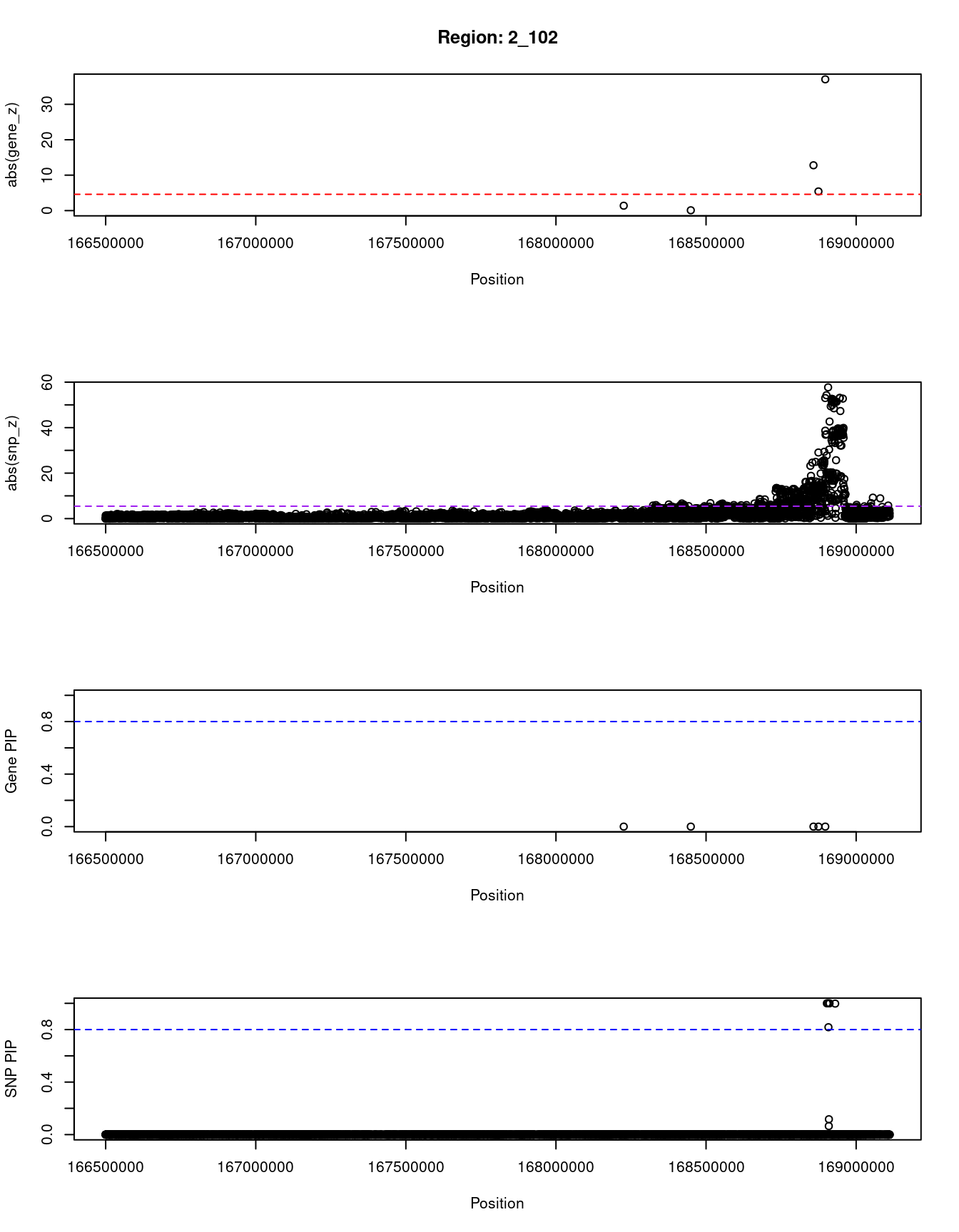
| Version | Author | Date |
|---|---|---|
| 0c9ef1c | wesleycrouse | 2021-09-08 |
[1] "Region: 3_104"
       genename region_tag susie_pip   mu2     PVE     z
12400 LINC02082      3_104     0.037  8.03 9.4e-07  1.08
10300    ACTRT3      3_104     0.024  5.19 3.9e-07 -1.27
9007     LRRC34      3_104     0.035  7.59 8.5e-07 -0.85
1170      MECOM      3_104     0.218 22.13 1.5e-05  2.61
165       SEC62      3_104     0.038  7.79 9.3e-07  0.70
9276     GPR160      3_104     0.025  4.73 3.7e-07 -0.23
9275       PHC3      3_104     0.038  8.32 9.9e-07 -1.29
7683      PRKCI      3_104     0.023  5.57 4.1e-07 -1.46
5117       SKIL      3_104     0.027  5.88 5.0e-07  0.94
230     SLC7A14      3_104     0.036  7.05 8.1e-07  0.12
7689     EIF5A2      3_104     0.027 20.53 1.7e-06 -6.97
7690     SLC2A2      3_104     0.029 77.64 7.0e-06 14.53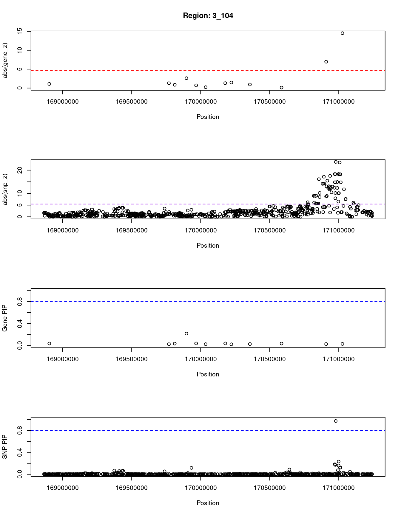
| Version | Author | Date |
|---|---|---|
| 0c9ef1c | wesleycrouse | 2021-09-08 |
[1] "Region: 7_32"
       genename region_tag susie_pip   mu2     PVE     z
2356      BLVRA       7_32     0.000  5.59 2.3e-11 -0.96
7904     STK17A       7_32     0.000 14.12 1.4e-10 -2.06
2355       COA1       7_32     0.000 30.26 1.6e-09 -3.41
589      MRPS24       7_32     0.000  9.69 1.4e-10  0.07
2357      URGCP       7_32     0.000  8.09 4.7e-11  3.05
1021     UBE2D4       7_32     0.000 36.98 2.1e-10 -6.51
12252 LINC00957       7_32     0.000 16.85 1.1e-10  4.64
5086       DBNL       7_32     0.000 14.05 9.5e-11  1.97
3767       POLM       7_32     0.000  8.33 6.2e-11 -1.04
2361      AEBP1       7_32     0.000 24.87 1.4e-10  6.75
2362      POLD2       7_32     0.000 13.00 1.3e-09  1.98
2366       YKT6       7_32     0.002 91.62 4.9e-07 11.82
547      CAMK2B       7_32     0.000 23.68 1.8e-09  1.65
258      NPC1L1       7_32     0.000  7.20 3.0e-11  1.71
5083      DDX56       7_32     0.000 10.65 9.4e-11 -1.61
7150      TMED4       7_32     0.000  7.57 3.1e-11 -1.02
2281       OGDH       7_32     0.000 22.66 1.3e-09 -2.16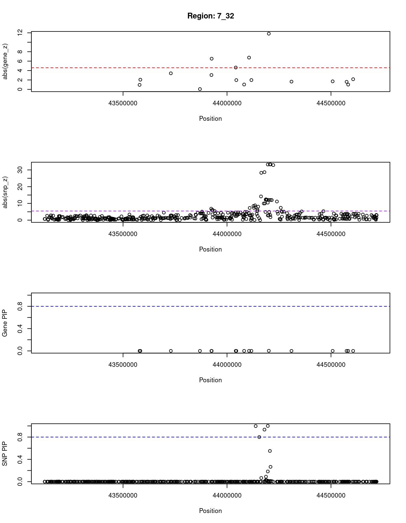
| Version | Author | Date |
|---|---|---|
| 0c9ef1c | wesleycrouse | 2021-09-08 |
[1] "Region: 14_45"
           genename region_tag susie_pip   mu2     PVE     z
12801  RP11-944C7.1      14_45     0.055 46.00 8.1e-06  7.47
487           FOXN3      14_45     0.051 84.06 1.4e-05 10.50
410            TDP1      14_45     0.076 10.28 2.5e-06 -1.89
5578        EFCAB11      14_45     0.048  4.78 7.4e-07  0.25
6685         KCNK13      14_45     0.099 10.52 3.3e-06  1.27
1726          PSMC1      14_45     0.055  6.01 1.1e-06  0.90
13496 RP11-471B22.3      14_45     0.048  4.67 7.1e-07 -0.23
11325         CALM1      14_45     0.122 12.81 5.0e-06  1.79
8113          TTC7B      14_45     0.057  6.23 1.1e-06 -0.77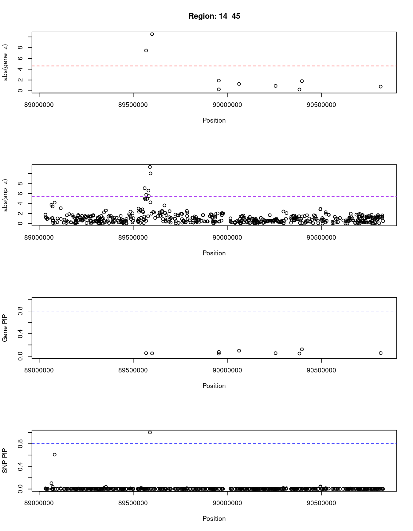
| Version | Author | Date |
|---|---|---|
| 0c9ef1c | wesleycrouse | 2021-09-08 |
[1] "Region: 2_16"
      genename region_tag susie_pip   mu2     PVE      z
8947     KCNK3       2_16     0.047  5.00 7.5e-07   0.01
7094      CIB4       2_16     0.048  5.45 8.4e-07   0.26
11762  SLC35F6       2_16     0.071  6.94 1.6e-06  -0.93
1164    MAPRE3       2_16     0.193 16.63 1.0e-05   4.46
3542   TMEM214       2_16     0.076 13.61 3.3e-06  -3.75
5339   EMILIN1       2_16     0.059  7.44 1.4e-06   2.83
5327       KHK       2_16     0.054 11.61 2.0e-06   3.39
5325    CGREF1       2_16     0.046  9.40 1.4e-06   2.31
6016     ABHD1       2_16     0.045  9.87 1.4e-06   3.80
5335      PREB       2_16     0.082 13.68 3.5e-06   2.51
5341    ATRAID       2_16     0.048 19.99 3.0e-06   4.77
5336    SLC5A6       2_16     0.043  9.58 1.3e-06  -2.97
1165       CAD       2_16     0.057 14.84 2.7e-06   3.50
5344    TRIM54       2_16     0.051 21.21 3.4e-06  -4.48
7740       UCN       2_16     0.045  8.10 1.1e-06   2.74
3132     SNX17       2_16     0.044  8.58 1.2e-06   2.78
3134     PPM1G       2_16     0.072 85.02 1.9e-05 -10.23
3128     NRBP1       2_16     0.096 90.27 2.8e-05 -10.47
7101   KRTCAP3       2_16     0.058 13.47 2.5e-06  -3.56
11298     GPN1       2_16     0.047 12.51 1.9e-06  -2.81
9562   CCDC121       2_16     0.085  8.25 2.2e-06   0.35
7106       BRE       2_16     0.044  6.09 8.5e-07  -1.65
8928      RBKS       2_16     0.044 33.84 4.7e-06  -6.85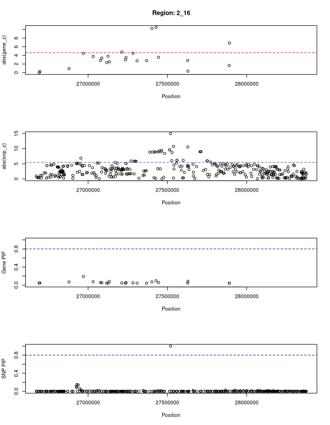
| Version | Author | Date |
|---|---|---|
| 0c9ef1c | wesleycrouse | 2021-09-08 |
SNPs with highest PIPs
#snps with PIP>0.8 or 20 highest PIPs
head(ctwas_snp_res[order(-ctwas_snp_res$susie_pip),report_cols_snps],
max(sum(ctwas_snp_res$susie_pip>0.8), 20))
id region_tag susie_pip mu2 PVE z
54769 rs79687284 1_108 1.000 113.61 3.6e-04 -12.08
75841 rs780093 2_16 1.000 194.86 6.2e-04 -14.95
114967 rs12692596 2_96 1.000 47.30 1.5e-04 -7.24
166279 rs148685409 3_57 1.000 1172.25 3.7e-03 2.99
176111 rs72964564 3_76 1.000 246.73 7.8e-04 16.88
196158 rs4234603 3_115 1.000 40.95 1.3e-04 -5.05
385952 rs10225316 7_15 1.000 46.39 1.5e-04 -7.51
396189 rs138917529 7_32 1.000 76.48 2.4e-04 10.45
435966 rs7012814 8_12 1.000 63.79 2.0e-04 9.18
531556 rs61856594 10_33 1.000 39.31 1.2e-04 6.23
550756 rs12244851 10_70 1.000 303.38 9.6e-04 -16.46
573941 rs2596407 11_29 1.000 72.48 2.3e-04 -9.98
648484 rs576674 13_10 1.000 107.51 3.4e-04 10.82
697477 rs35889227 14_45 1.000 118.99 3.8e-04 11.34
871531 rs2232318 2_102 1.000 134.27 4.3e-04 -2.07
871537 rs560887 2_102 1.000 2891.53 9.2e-03 -57.71
871547 rs71397670 2_102 1.000 851.49 2.7e-03 -42.67
287543 rs12189028 5_45 0.999 36.68 1.2e-04 5.08
480498 rs10758593 9_4 0.999 73.13 2.3e-04 -8.64
559062 rs3842727 11_2 0.999 104.42 3.3e-04 8.57
897929 rs2168101 11_6 0.999 69.48 2.2e-04 8.60
54778 rs3754140 1_108 0.998 59.17 1.9e-04 10.01
235214 rs11728350 4_69 0.998 43.88 1.4e-04 -6.68
871618 rs56100844 2_102 0.998 159.91 5.1e-04 17.86
396169 rs17769733 7_32 0.997 176.30 5.6e-04 7.76
562709 rs34718245 11_9 0.997 32.87 1.0e-04 5.37
758800 rs28489441 17_15 0.997 33.77 1.1e-04 5.83
513302 rs115478735 9_71 0.996 84.06 2.7e-04 -9.52
663129 rs1327315 13_40 0.995 36.75 1.2e-04 7.02
323022 rs55792466 6_7 0.994 100.29 3.2e-04 9.67
487738 rs572168822 9_16 0.994 42.16 1.3e-04 6.61
815325 rs34783010 19_32 0.993 35.23 1.1e-04 6.40
639602 rs4765221 12_76 0.990 34.68 1.1e-04 -5.80
550208 rs11195508 10_70 0.987 61.70 1.9e-04 10.76
559067 rs10743152 11_2 0.986 42.41 1.3e-04 -1.91
413168 rs4729755 7_63 0.978 26.99 8.4e-05 -4.96
487733 rs1333045 9_16 0.977 41.66 1.3e-04 -6.62
191001 rs10653660 3_104 0.971 360.84 1.1e-03 23.54
755 rs60330317 1_2 0.969 37.90 1.2e-04 6.18
469203 rs4433184 8_78 0.969 55.62 1.7e-04 -4.78
646794 rs60353775 13_7 0.969 84.48 2.6e-04 -9.78
707721 rs12912777 15_13 0.969 25.96 8.0e-05 -3.77
631101 rs6538805 12_58 0.967 32.57 1.0e-04 6.74
478456 rs4977218 8_94 0.964 30.86 9.4e-05 5.34
174145 rs9875598 3_73 0.962 27.90 8.5e-05 5.10
573841 rs7111517 11_28 0.955 39.53 1.2e-04 6.64
514592 rs28624681 9_73 0.946 53.45 1.6e-04 -7.55
704198 rs35767992 15_4 0.946 24.97 7.5e-05 -4.72
675057 rs80081165 13_62 0.943 25.89 7.8e-05 -4.82
396181 rs10259649 7_32 0.934 410.04 1.2e-03 -28.65
573644 rs117396352 11_28 0.934 27.94 8.3e-05 -4.93
760309 rs543720569 17_18 0.930 45.39 1.3e-04 7.03
336714 rs62396405 6_30 0.916 25.91 7.5e-05 4.78
456808 rs10957704 8_54 0.912 25.30 7.3e-05 -4.68
642634 rs1882297 12_82 0.909 40.60 1.2e-04 -6.47
575545 rs182512331 11_31 0.902 28.19 8.1e-05 5.05
154708 rs3172494 3_34 0.899 26.97 7.7e-05 5.09
837659 rs6026545 20_34 0.896 32.57 9.3e-05 -5.72
563641 rs117720468 11_11 0.895 45.26 1.3e-04 -6.82
801634 rs10410896 19_4 0.879 28.13 7.9e-05 -5.04
34659 rs893230 1_72 0.878 41.13 1.1e-04 7.56
359234 rs118126621 6_73 0.872 25.88 7.2e-05 -4.67
575127 rs139913257 11_30 0.864 32.42 8.9e-05 5.63
798417 rs41404946 18_44 0.855 25.17 6.8e-05 -4.56
365712 rs112388031 6_87 0.854 25.75 7.0e-05 4.65
257349 rs62332172 4_113 0.832 25.28 6.7e-05 -4.54
398525 rs11763778 7_36 0.830 45.69 1.2e-04 7.61
19026 rs6699568 1_42 0.826 28.09 7.4e-05 -5.02
578656 rs7941126 11_36 0.826 32.53 8.5e-05 5.63
871539 rs492594 2_102 0.818 926.56 2.4e-03 -17.82
663480 rs79317015 13_40 0.808 25.64 6.6e-05 -4.40
195698 rs73185688 3_114 0.803 25.85 6.6e-05 -4.69
580686 rs11603349 11_41 0.803 45.41 1.2e-04 6.78
609282 rs12582270 12_17 0.803 26.58 6.8e-05 4.72SNPs with largest effect sizes
#plot PIP vs effect size
plot(ctwas_snp_res$susie_pip, ctwas_snp_res$mu2, xlab="PIP", ylab="mu^2", main="SNP PIPs vs Effect Size")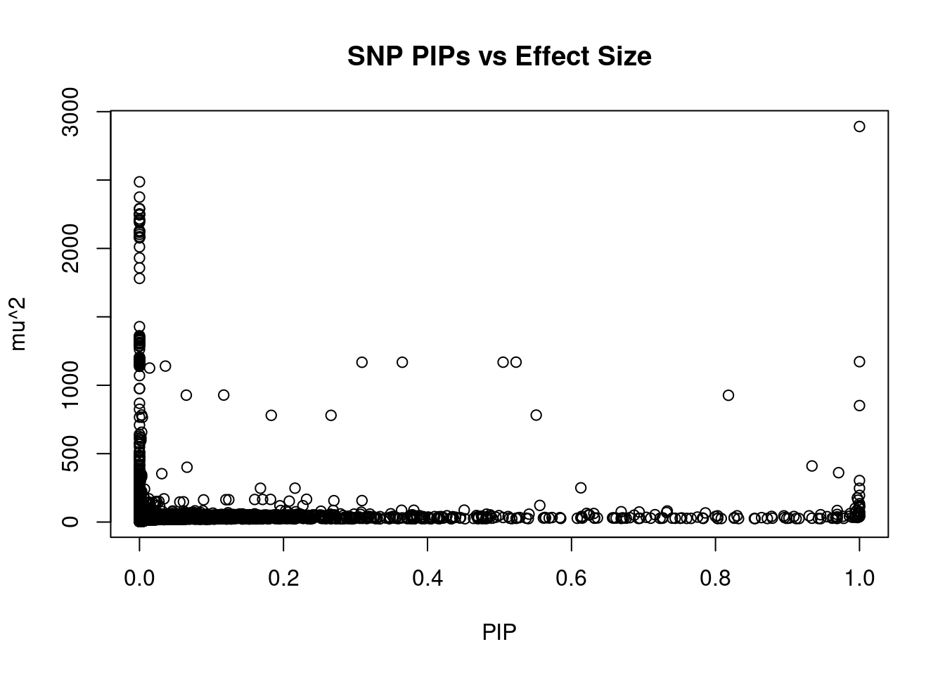
| Version | Author | Date |
|---|---|---|
| 0c9ef1c | wesleycrouse | 2021-09-08 |
#SNPs with 50 largest effect sizes
head(ctwas_snp_res[order(-ctwas_snp_res$mu2),report_cols_snps],50)
id region_tag susie_pip mu2 PVE z
871537 rs560887 2_102 1 2891.53 9.2e-03 -57.71
871526 rs573225 2_102 0 2487.13 6.5e-12 -54.23
871514 rs13431652 2_102 0 2375.41 1.2e-11 53.00
871671 rs853787 2_102 0 2291.40 5.2e-07 -53.06
871668 rs853789 2_102 0 2288.31 4.7e-07 -53.04
871563 rs537183 2_102 0 2252.17 1.4e-10 -52.66
871698 rs853777 2_102 0 2251.00 2.8e-07 -52.75
871561 rs563694 2_102 0 2246.54 1.4e-10 -52.60
871586 rs557462 2_102 0 2246.40 1.3e-10 -52.60
871565 rs502570 2_102 0 2215.18 1.1e-10 -52.14
871579 rs475612 2_102 0 2204.14 5.6e-11 -52.14
871582 rs518598 2_102 0 2203.57 5.5e-11 -52.13
871575 rs578763 2_102 0 2200.84 6.8e-11 -52.08
871570 rs580670 2_102 0 2188.97 6.1e-11 -51.95
871614 rs508506 2_102 0 2129.36 2.6e-10 -51.54
871605 rs569829 2_102 0 2126.47 2.3e-10 -51.52
871626 rs494874 2_102 0 2125.89 3.0e-10 -51.48
871572 rs580613 2_102 0 2124.83 5.2e-11 -51.23
871633 rs552976 2_102 0 2117.73 3.0e-10 -51.36
871571 rs580639 2_102 0 2102.86 1.3e-10 -51.53
871601 rs486981 2_102 0 2086.01 1.1e-10 -51.05
871602 rs485094 2_102 0 2084.58 1.0e-10 -51.04
871608 rs566879 2_102 0 2083.38 1.0e-10 -51.03
871607 rs579060 2_102 0 2081.26 1.0e-10 -51.00
871606 rs569805 2_102 0 2077.34 1.1e-10 -50.95
871584 rs796703396 2_102 0 2011.75 1.3e-12 -49.98
871559 rs504979 2_102 0 1931.18 1.2e-12 -49.37
871603 rs484066 2_102 0 1858.06 8.7e-13 -48.49
871677 rs71397677 2_102 0 1781.15 1.6e-11 -47.29
871516 rs12475700 2_102 0 1428.38 1.6e-14 -38.64
871646 rs2544360 2_102 0 1362.03 1.8e-12 -39.60
871642 rs508743 2_102 0 1359.01 1.2e-12 39.58
871673 rs862662 2_102 0 1350.59 1.2e-12 -39.50
871645 rs79933700 2_102 0 1349.57 1.1e-12 39.46
871692 rs1101532 2_102 0 1342.83 1.3e-12 -39.54
871652 rs2685807 2_102 0 1335.53 9.9e-13 -39.24
871666 rs853791 2_102 0 1331.93 8.6e-13 -39.21
871663 rs2250677 2_102 0 1326.14 7.7e-13 -39.12
871624 rs531772 2_102 0 1313.44 1.5e-13 -38.74
871597 rs575671 2_102 0 1309.13 1.4e-13 -38.66
871701 rs853775 2_102 0 1307.72 6.8e-13 -39.04
871638 rs567074 2_102 0 1303.38 3.4e-13 38.66
871595 rs473351 2_102 0 1303.02 1.2e-13 -38.57
871577 rs500432 2_102 0 1289.60 3.5e-14 -37.99
871682 rs853781 2_102 0 1287.52 3.7e-13 -38.77
871681 rs853782 2_102 0 1285.16 3.4e-13 -38.75
871703 rs853773 2_102 0 1262.44 4.3e-12 -39.87
871670 rs853788 2_102 0 1204.98 4.4e-14 -37.47
871674 rs853785 2_102 0 1203.07 4.2e-14 -37.45
871691 rs35351007 2_102 0 1196.79 8.4e-14 -37.70SNPs with highest PVE
#SNPs with 50 highest pve
head(ctwas_snp_res[order(-ctwas_snp_res$PVE),report_cols_snps],50)
id region_tag susie_pip mu2 PVE z
871537 rs560887 2_102 1.000 2891.53 0.00920 -57.71
166279 rs148685409 3_57 1.000 1172.25 0.00370 2.99
871547 rs71397670 2_102 1.000 851.49 0.00270 -42.67
871539 rs492594 2_102 0.818 926.56 0.00240 -17.82
166281 rs1436648 3_57 0.505 1168.51 0.00190 3.09
166282 rs7619398 3_57 0.523 1168.85 0.00190 3.08
166283 rs2256473 3_57 0.365 1168.10 0.00140 3.06
396194 rs917793 7_32 0.551 781.75 0.00140 -33.28
396181 rs10259649 7_32 0.934 410.04 0.00120 -28.65
166280 rs2575789 3_57 0.309 1167.97 0.00110 3.06
191001 rs10653660 3_104 0.971 360.84 0.00110 23.54
550756 rs12244851 10_70 1.000 303.38 0.00096 -16.46
176111 rs72964564 3_76 1.000 246.73 0.00078 16.88
396198 rs2908282 7_32 0.266 779.97 0.00066 -33.26
75841 rs780093 2_16 1.000 194.86 0.00062 -14.95
396169 rs17769733 7_32 0.997 176.30 0.00056 7.76
871618 rs56100844 2_102 0.998 159.91 0.00051 17.86
386012 rs1974619 7_15 0.613 250.08 0.00049 -16.89
396188 rs4607517 7_32 0.183 780.12 0.00045 -33.23
871531 rs2232318 2_102 1.000 134.27 0.00043 -2.07
697477 rs35889227 14_45 1.000 118.99 0.00038 11.34
54769 rs79687284 1_108 1.000 113.61 0.00036 -12.08
648484 rs576674 13_10 1.000 107.51 0.00034 10.82
871543 rs567243 2_102 0.117 928.24 0.00034 -17.95
559062 rs3842727 11_2 0.999 104.42 0.00033 8.57
323022 rs55792466 6_7 0.994 100.29 0.00032 9.67
513302 rs115478735 9_71 0.996 84.06 0.00027 -9.52
646794 rs60353775 13_7 0.969 84.48 0.00026 -9.78
396189 rs138917529 7_32 1.000 76.48 0.00024 10.45
480498 rs10758593 9_4 0.999 73.13 0.00023 -8.64
573941 rs2596407 11_29 1.000 72.48 0.00023 -9.98
897929 rs2168101 11_6 0.999 69.48 0.00022 8.60
292807 rs17085655 5_56 0.556 121.58 0.00021 11.48
435966 rs7012814 8_12 1.000 63.79 0.00020 9.18
54778 rs3754140 1_108 0.998 59.17 0.00019 10.01
550208 rs11195508 10_70 0.987 61.70 0.00019 10.76
550750 rs117764423 10_70 0.733 80.91 0.00019 5.24
871542 rs570876 2_102 0.065 927.59 0.00019 -18.01
327614 rs2206734 6_15 0.786 66.67 0.00017 -8.26
386010 rs10228796 7_15 0.216 247.61 0.00017 -16.82
469203 rs4433184 8_78 0.969 55.62 0.00017 -4.78
261433 rs12499544 4_119 0.732 70.29 0.00016 8.39
469227 rs28529793 8_78 0.694 73.68 0.00016 6.80
514592 rs28624681 9_73 0.946 53.45 0.00016 -7.55
828221 rs111405491 20_16 0.669 75.51 0.00016 8.97
114967 rs12692596 2_96 1.000 47.30 0.00015 -7.24
166269 rs138788521 3_57 0.309 156.77 0.00015 -3.55
385952 rs10225316 7_15 1.000 46.39 0.00015 -7.51
235214 rs11728350 4_69 0.998 43.88 0.00014 -6.68
166264 rs192265655 3_57 0.270 156.24 0.00013 -3.52SNPs with largest z scores
#SNPs with 50 largest z scores
head(ctwas_snp_res[order(-abs(ctwas_snp_res$z)),report_cols_snps],50)
id region_tag susie_pip mu2 PVE z
871537 rs560887 2_102 1 2891.53 9.2e-03 -57.71
871526 rs573225 2_102 0 2487.13 6.5e-12 -54.23
871671 rs853787 2_102 0 2291.40 5.2e-07 -53.06
871668 rs853789 2_102 0 2288.31 4.7e-07 -53.04
871514 rs13431652 2_102 0 2375.41 1.2e-11 53.00
871698 rs853777 2_102 0 2251.00 2.8e-07 -52.75
871563 rs537183 2_102 0 2252.17 1.4e-10 -52.66
871561 rs563694 2_102 0 2246.54 1.4e-10 -52.60
871586 rs557462 2_102 0 2246.40 1.3e-10 -52.60
871565 rs502570 2_102 0 2215.18 1.1e-10 -52.14
871579 rs475612 2_102 0 2204.14 5.6e-11 -52.14
871582 rs518598 2_102 0 2203.57 5.5e-11 -52.13
871575 rs578763 2_102 0 2200.84 6.8e-11 -52.08
871570 rs580670 2_102 0 2188.97 6.1e-11 -51.95
871614 rs508506 2_102 0 2129.36 2.6e-10 -51.54
871571 rs580639 2_102 0 2102.86 1.3e-10 -51.53
871605 rs569829 2_102 0 2126.47 2.3e-10 -51.52
871626 rs494874 2_102 0 2125.89 3.0e-10 -51.48
871633 rs552976 2_102 0 2117.73 3.0e-10 -51.36
871572 rs580613 2_102 0 2124.83 5.2e-11 -51.23
871601 rs486981 2_102 0 2086.01 1.1e-10 -51.05
871602 rs485094 2_102 0 2084.58 1.0e-10 -51.04
871608 rs566879 2_102 0 2083.38 1.0e-10 -51.03
871607 rs579060 2_102 0 2081.26 1.0e-10 -51.00
871606 rs569805 2_102 0 2077.34 1.1e-10 -50.95
871584 rs796703396 2_102 0 2011.75 1.3e-12 -49.98
871559 rs504979 2_102 0 1931.18 1.2e-12 -49.37
871603 rs484066 2_102 0 1858.06 8.7e-13 -48.49
871677 rs71397677 2_102 0 1781.15 1.6e-11 -47.29
871547 rs71397670 2_102 1 851.49 2.7e-03 -42.67
871703 rs853773 2_102 0 1262.44 4.3e-12 -39.87
871646 rs2544360 2_102 0 1362.03 1.8e-12 -39.60
871642 rs508743 2_102 0 1359.01 1.2e-12 39.58
871692 rs1101532 2_102 0 1342.83 1.3e-12 -39.54
871673 rs862662 2_102 0 1350.59 1.2e-12 -39.50
871645 rs79933700 2_102 0 1349.57 1.1e-12 39.46
871652 rs2685807 2_102 0 1335.53 9.9e-13 -39.24
871666 rs853791 2_102 0 1331.93 8.6e-13 -39.21
871663 rs2250677 2_102 0 1326.14 7.7e-13 -39.12
871701 rs853775 2_102 0 1307.72 6.8e-13 -39.04
871682 rs853781 2_102 0 1287.52 3.7e-13 -38.77
871681 rs853782 2_102 0 1285.16 3.4e-13 -38.75
871624 rs531772 2_102 0 1313.44 1.5e-13 -38.74
871597 rs575671 2_102 0 1309.13 1.4e-13 -38.66
871638 rs567074 2_102 0 1303.38 3.4e-13 38.66
871516 rs12475700 2_102 0 1428.38 1.6e-14 -38.64
871595 rs473351 2_102 0 1303.02 1.2e-13 -38.57
871577 rs500432 2_102 0 1289.60 3.5e-14 -37.99
871691 rs35351007 2_102 0 1196.79 8.4e-14 -37.70
871694 rs853778 2_102 0 1193.20 3.6e-14 -37.54Gene set enrichment for genes with PIP>0.8
#GO enrichment analysis
library(enrichR)
Welcome to enrichR
Checking connection ... Enrichr ... Connection is Live!
FlyEnrichr ... Connection is available!
WormEnrichr ... Connection is available!
YeastEnrichr ... Connection is available!
FishEnrichr ... Connection is available!dbs <- c("GO_Biological_Process_2021", "GO_Cellular_Component_2021", "GO_Molecular_Function_2021")
genes <- ctwas_gene_res$genename[ctwas_gene_res$susie_pip>0.8]
#number of genes for gene set enrichment
length(genes)[1] 6if (length(genes)>0){
GO_enrichment <- enrichr(genes, dbs)
for (db in dbs){
print(db)
df <- GO_enrichment[[db]]
df <- df[df$Adjusted.P.value<0.05,c("Term", "Overlap", "Adjusted.P.value", "Genes")]
print(df)
}
#DisGeNET enrichment
# devtools::install_bitbucket("ibi_group/disgenet2r")
library(disgenet2r)
disgenet_api_key <- get_disgenet_api_key(
email = "wesleycrouse@gmail.com",
password = "uchicago1" )
Sys.setenv(DISGENET_API_KEY= disgenet_api_key)
res_enrich <-disease_enrichment(entities=genes, vocabulary = "HGNC",
database = "CURATED" )
df <- res_enrich@qresult[1:10, c("Description", "FDR", "Ratio", "BgRatio")]
print(df)
#WebGestalt enrichment
library(WebGestaltR)
background <- ctwas_gene_res$genename
#listGeneSet()
databases <- c("pathway_KEGG", "disease_GLAD4U", "disease_OMIM")
enrichResult <- WebGestaltR(enrichMethod="ORA", organism="hsapiens",
interestGene=genes, referenceGene=background,
enrichDatabase=databases, interestGeneType="genesymbol",
referenceGeneType="genesymbol", isOutput=F)
print(enrichResult[,c("description", "size", "overlap", "FDR", "database", "userId")])
}Uploading data to Enrichr... Done.
Querying GO_Biological_Process_2021... Done.
Querying GO_Cellular_Component_2021... Done.
Querying GO_Molecular_Function_2021... Done.
Parsing results... Done.
[1] "GO_Biological_Process_2021"
Term Overlap
1 lipid droplet formation (GO:0140042) 1/10
2 cyclooxygenase pathway (GO:0019371) 1/11
3 prostanoid biosynthetic process (GO:0046457) 1/15
4 prostaglandin biosynthetic process (GO:0001516) 1/19
5 chaperone-mediated protein complex assembly (GO:0051131) 1/22
6 lipid droplet organization (GO:0034389) 1/22
7 chaperone cofactor-dependent protein refolding (GO:0051085) 1/26
8 telomere maintenance via telomerase (GO:0007004) 1/29
9 positive regulation of phosphate metabolic process (GO:0045937) 1/30
10 RNA-dependent DNA biosynthetic process (GO:0006278) 1/30
11 'de novo' posttranslational protein folding (GO:0051084) 1/31
12 prostaglandin metabolic process (GO:0006693) 1/31
13 positive regulation of telomerase activity (GO:0051973) 1/34
14 telomere maintenance via telomere lengthening (GO:0010833) 1/36
15 regulation of telomerase activity (GO:0051972) 1/46
16 telomere organization (GO:0032200) 1/47
17 telomere maintenance (GO:0000723) 1/56
18 Rho protein signal transduction (GO:0007266) 1/56
19 arachidonic acid metabolic process (GO:0019369) 1/57
20 positive regulation of DNA biosynthetic process (GO:2000573) 1/61
21 regulation of actin filament-based process (GO:0032970) 1/73
22 regulation of cellular response to heat (GO:1900034) 1/79
Adjusted.P.value Genes
1 0.03379435 SMIM22
2 0.03379435 PTGES3
3 0.03379435 PTGES3
4 0.03379435 PTGES3
5 0.03379435 PTGES3
6 0.03379435 SMIM22
7 0.03379435 PTGES3
8 0.03379435 PTGES3
9 0.03379435 PTGES3
10 0.03379435 PTGES3
11 0.03379435 PTGES3
12 0.03379435 PTGES3
13 0.03379435 PTGES3
14 0.03379435 PTGES3
15 0.03855236 PTGES3
16 0.03855236 PTGES3
17 0.03932348 PTGES3
18 0.03932348 CTNNAL1
19 0.03932348 PTGES3
20 0.03995890 PTGES3
21 0.04547434 SMIM22
22 0.04693986 PTGES3
[1] "GO_Cellular_Component_2021"
Term Overlap
1 post-mRNA release spliceosomal complex (GO:0071014) 1/11
Adjusted.P.value Genes
1 0.009887477 CWF19L1
[1] "GO_Molecular_Function_2021"
Term Overlap
1 RNA-directed DNA polymerase activity (GO:0003964) 1/6
2 telomerase activity (GO:0003720) 1/6
3 DNA polymerase binding (GO:0070182) 1/18
4 Hsp90 protein binding (GO:0051879) 1/35
Adjusted.P.value Genes
1 0.006295943 PTGES3
2 0.006295943 PTGES3
3 0.012573087 PTGES3
4 0.018296889 PTGES3C15orf52 gene(s) from the input list not found in DisGeNET CURATEDCTNNAL1 gene(s) from the input list not found in DisGeNET CURATEDSMIM22 gene(s) from the input list not found in DisGeNET CURATED Description FDR Ratio
15 SPINOCEREBELLAR ATAXIA, AUTOSOMAL RECESSIVE 17 0.004638219 1/3
3 Adult T-Cell Lymphoma/Leukemia 0.013480779 1/3
4 Ataxia, Spinocerebellar 0.013480779 1/3
5 Encephalopathy, Toxic 0.013480779 1/3
6 Toxic Encephalitis 0.013480779 1/3
7 Neurotoxicity Syndromes 0.013480779 1/3
8 Spinocerebellar Ataxia Type 1 0.013480779 1/3
9 Spinocerebellar Ataxia Type 2 0.013480779 1/3
10 Spinocerebellar Ataxia Type 4 0.013480779 1/3
11 Spinocerebellar Ataxia Type 5 0.013480779 1/3
BgRatio
15 1/9703
3 31/9703
4 34/9703
5 29/9703
6 29/9703
7 29/9703
8 34/9703
9 34/9703
10 35/9703
11 34/9703******************************************
* *
* Welcome to WebGestaltR ! *
* *
******************************************Loading the functional categories...
Loading the ID list...
Loading the reference list...
Performing the enrichment analysis...Warning in oraEnrichment(interestGeneList, referenceGeneList, geneSet,
minNum = minNum, : No significant gene set is identified based on FDR 0.05!NULLSensitivity, specificity and precision for silver standard genes
library("readxl")

known_annotations <- read_xlsx("data/summary_known_genes_annotations.xlsx", sheet="Glucose")
known_annotations <- unique(known_annotations$`Gene Symbol`)

unrelated_genes <- ctwas_gene_res$genename[!(ctwas_gene_res$genename %in% known_annotations)]

#number of genes in known annotations
print(length(known_annotations))
[1] 87#number of genes in known annotations with imputed expression
print(sum(known_annotations %in% ctwas_gene_res$genename))[1] 46#assign ctwas, TWAS, and bystander genes
ctwas_genes <- ctwas_gene_res$genename[ctwas_gene_res$susie_pip>0.8]
twas_genes <- ctwas_gene_res$genename[abs(ctwas_gene_res$z)>sig_thresh]
novel_genes <- ctwas_genes[!(ctwas_genes %in% twas_genes)]
#significance threshold for TWAS
print(sig_thresh)[1] 4.600359#number of ctwas genes
length(ctwas_genes)[1] 6#number of TWAS genes
length(twas_genes)[1] 87#show novel genes (ctwas genes with not in TWAS genes)
ctwas_gene_res[ctwas_gene_res$genename %in% novel_genes,report_cols] genename region_tag susie_pip mu2 PVE z
1451 CWF19L1 10_64 0.832 18.41 4.9e-05 -4.12
2726 PTGES3 12_35 0.909 18.45 5.3e-05 4.17
10780 C15orf52 15_14 0.848 21.20 5.7e-05 -4.58
13108 SMIM22 16_4 0.913 18.54 5.4e-05 4.21#sensitivity / recall
sensitivity <- rep(NA,2)
names(sensitivity) <- c("ctwas", "TWAS")
sensitivity["ctwas"] <- sum(ctwas_genes %in% known_annotations)/length(known_annotations)
sensitivity["TWAS"] <- sum(twas_genes %in% known_annotations)/length(known_annotations)
sensitivity ctwas TWAS
0.00000000 0.02298851 #specificity
specificity <- rep(NA,2)
names(specificity) <- c("ctwas", "TWAS")
specificity["ctwas"] <- sum(!(unrelated_genes %in% ctwas_genes))/length(unrelated_genes)
specificity["TWAS"] <- sum(!(unrelated_genes %in% twas_genes))/length(unrelated_genes)
specificity ctwas TWAS
0.9994919 0.9928021 #precision / PPV
precision <- rep(NA,2)
names(precision) <- c("ctwas", "TWAS")
precision["ctwas"] <- sum(ctwas_genes %in% known_annotations)/length(ctwas_genes)
precision["TWAS"] <- sum(twas_genes %in% known_annotations)/length(twas_genes)
precision ctwas TWAS
0.00000000 0.02298851 #ROC curves
pip_range <- (0:1000)/1000
sensitivity <- rep(NA, length(pip_range))
specificity <- rep(NA, length(pip_range))
for (index in 1:length(pip_range)){
pip <- pip_range[index]
ctwas_genes <- ctwas_gene_res$genename[ctwas_gene_res$susie_pip>=pip]
sensitivity[index] <- sum(ctwas_genes %in% known_annotations)/length(known_annotations)
specificity[index] <- sum(!(unrelated_genes %in% ctwas_genes))/length(unrelated_genes)
}
plot(1-specificity, sensitivity, type="l", xlim=c(0,1), ylim=c(0,1))
sig_thresh_range <- seq(from=0, to=max(abs(ctwas_gene_res$z)), length.out=length(pip_range))
for (index in 1:length(sig_thresh_range)){
sig_thresh_plot <- sig_thresh_range[index]
twas_genes <- ctwas_gene_res$genename[abs(ctwas_gene_res$z)>=sig_thresh_plot]
sensitivity[index] <- sum(twas_genes %in% known_annotations)/length(known_annotations)
specificity[index] <- sum(!(unrelated_genes %in% twas_genes))/length(unrelated_genes)
}
lines(1-specificity, sensitivity, xlim=c(0,1), ylim=c(0,1), col="red", lty=2)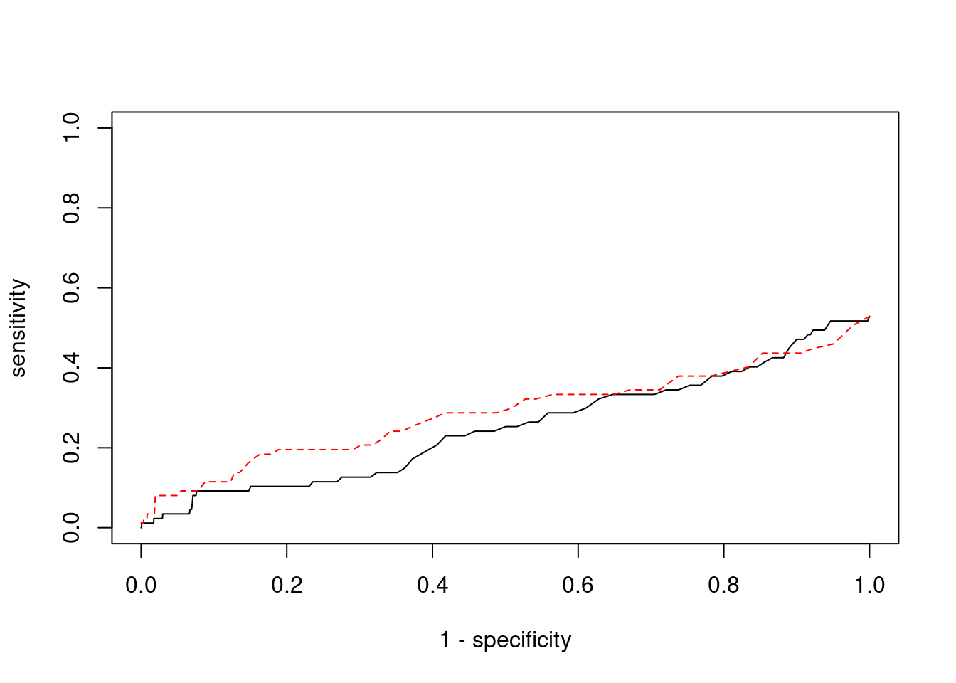
| Version | Author | Date |
|---|---|---|
| 0c9ef1c | wesleycrouse | 2021-09-08 |
Sensitivity, specificity and precision for silver standard genes - bystanders only
This section first uses all silver standard genes to identify bystander genes within 1Mb. The silver standard and bystander gene lists are then subset to only genes with imputed expression in this analysis. Then, the ctwas and TWAS gene lists from this analysis are subset to only genes that are in the (subset) silver standard and bystander genes. These gene lists are then used to compute sensitivity, specificity and precision for ctwas and TWAS.
library(biomaRt)
library(GenomicRanges)Loading required package: stats4Loading required package: BiocGenericsLoading required package: parallel
Attaching package: 'BiocGenerics'The following objects are masked from 'package:parallel':
clusterApply, clusterApplyLB, clusterCall, clusterEvalQ,
clusterExport, clusterMap, parApply, parCapply, parLapply,
parLapplyLB, parRapply, parSapply, parSapplyLBThe following objects are masked from 'package:stats':
IQR, mad, sd, var, xtabsThe following objects are masked from 'package:base':
anyDuplicated, append, as.data.frame, basename, cbind,
colnames, dirname, do.call, duplicated, eval, evalq, Filter,
Find, get, grep, grepl, intersect, is.unsorted, lapply, Map,
mapply, match, mget, order, paste, pmax, pmax.int, pmin,
pmin.int, Position, rank, rbind, Reduce, rownames, sapply,
setdiff, sort, table, tapply, union, unique, unsplit, which,
which.max, which.minLoading required package: S4Vectors
Attaching package: 'S4Vectors'The following object is masked from 'package:base':
expand.gridLoading required package: IRangesLoading required package: GenomeInfoDbensembl <- useEnsembl(biomart="ENSEMBL_MART_ENSEMBL", dataset="hsapiens_gene_ensembl")
G_list <- getBM(filters= "chromosome_name", attributes= c("hgnc_symbol","chromosome_name","start_position","end_position","gene_biotype"), values=1:22, mart=ensembl)
G_list <- G_list[G_list$hgnc_symbol!="",]
G_list <- G_list[G_list$gene_biotype %in% c("protein_coding","lncRNA"),]
G_list$start <- G_list$start_position
G_list$end <- G_list$end_position
G_list_granges <- makeGRangesFromDataFrame(G_list, keep.extra.columns=T)
known_annotations_positions <- G_list[G_list$hgnc_symbol %in% known_annotations,]
half_window <- 1000000
known_annotations_positions$start <- known_annotations_positions$start_position - half_window
known_annotations_positions$end <- known_annotations_positions$end_position + half_window
known_annotations_positions$start[known_annotations_positions$start<1] <- 1
known_annotations_granges <- makeGRangesFromDataFrame(known_annotations_positions, keep.extra.columns=T)
bystanders <- findOverlaps(known_annotations_granges,G_list_granges)
bystanders <- unique(subjectHits(bystanders))
bystanders <- G_list$hgnc_symbol[bystanders]
bystanders <- bystanders[!(bystanders %in% known_annotations)]
unrelated_genes <- bystanders
#number of genes in known annotations
print(length(known_annotations))[1] 87#number of genes in known annotations with imputed expression
print(sum(known_annotations %in% ctwas_gene_res$genename))[1] 46#number of bystander genes
print(length(unrelated_genes))[1] 1944#number of bystander genes with imputed expression
print(sum(unrelated_genes %in% ctwas_gene_res$genename))[1] 1016#remove genes without imputed expression from gene lists
known_annotations <- known_annotations[known_annotations %in% ctwas_gene_res$genename]
unrelated_genes <- unrelated_genes[unrelated_genes %in% ctwas_gene_res$genename]
#assign ctwas and TWAS genes
ctwas_genes <- ctwas_gene_res$genename[ctwas_gene_res$susie_pip>0.8]
twas_genes <- ctwas_gene_res$genename[abs(ctwas_gene_res$z)>sig_thresh]
#significance threshold for TWAS
print(sig_thresh)[1] 4.600359#number of ctwas genes
length(ctwas_genes)[1] 6#number of ctwas genes in known annotations or bystanders
sum(ctwas_genes %in% c(known_annotations, unrelated_genes))[1] 0#number of ctwas genes
length(twas_genes)[1] 87#number of TWAS genes
sum(twas_genes %in% c(known_annotations, unrelated_genes))[1] 21#remove genes not in known or bystander lists from results
ctwas_genes <- ctwas_genes[ctwas_genes %in% c(known_annotations, unrelated_genes)]
twas_genes <- twas_genes[twas_genes %in% c(known_annotations, unrelated_genes)]
#sensitivity / recall
sensitivity <- rep(NA,2)
names(sensitivity) <- c("ctwas", "TWAS")
sensitivity["ctwas"] <- sum(ctwas_genes %in% known_annotations)/length(known_annotations)
sensitivity["TWAS"] <- sum(twas_genes %in% known_annotations)/length(known_annotations)
sensitivity
ctwas TWAS
0.00000000 0.04347826 #specificity
specificity <- rep(NA,2)
names(specificity) <- c("ctwas", "TWAS")
specificity["ctwas"] <- sum(!(unrelated_genes %in% ctwas_genes))/length(unrelated_genes)
specificity["TWAS"] <- sum(!(unrelated_genes %in% twas_genes))/length(unrelated_genes)
specificity ctwas TWAS
1.0000000 0.9812992 #precision / PPV
precision <- rep(NA,2)
names(precision) <- c("ctwas", "TWAS")
precision["ctwas"] <- sum(ctwas_genes %in% known_annotations)/length(ctwas_genes)
precision["TWAS"] <- sum(twas_genes %in% known_annotations)/length(twas_genes)
precision ctwas TWAS
NaN 0.0952381
sessionInfo()R version 3.6.1 (2019-07-05)
Platform: x86_64-pc-linux-gnu (64-bit)
Running under: Scientific Linux 7.4 (Nitrogen)
Matrix products: default
BLAS/LAPACK: /software/openblas-0.2.19-el7-x86_64/lib/libopenblas_haswellp-r0.2.19.so
locale:
[1] LC_CTYPE=en_US.UTF-8 LC_NUMERIC=C
[3] LC_TIME=en_US.UTF-8 LC_COLLATE=en_US.UTF-8
[5] LC_MONETARY=en_US.UTF-8 LC_MESSAGES=en_US.UTF-8
[7] LC_PAPER=en_US.UTF-8 LC_NAME=C
[9] LC_ADDRESS=C LC_TELEPHONE=C
[11] LC_MEASUREMENT=en_US.UTF-8 LC_IDENTIFICATION=C
attached base packages:
[1] parallel stats4 stats graphics grDevices utils datasets
[8] methods base
other attached packages:
[1] GenomicRanges_1.36.0 GenomeInfoDb_1.20.0 IRanges_2.18.1
[4] S4Vectors_0.22.1 BiocGenerics_0.30.0 biomaRt_2.40.1
[7] readxl_1.3.1 WebGestaltR_0.4.4 disgenet2r_0.99.2
[10] enrichR_3.0 cowplot_1.0.0 ggplot2_3.3.3
loaded via a namespace (and not attached):
[1] bitops_1.0-6 fs_1.3.1 bit64_4.0.5
[4] doParallel_1.0.16 progress_1.2.2 httr_1.4.1
[7] rprojroot_2.0.2 tools_3.6.1 doRNG_1.8.2
[10] utf8_1.2.1 R6_2.5.0 DBI_1.1.1
[13] colorspace_1.4-1 withr_2.4.1 tidyselect_1.1.0
[16] prettyunits_1.0.2 bit_4.0.4 curl_3.3
[19] compiler_3.6.1 git2r_0.26.1 Biobase_2.44.0
[22] labeling_0.3 scales_1.1.0 readr_1.4.0
[25] stringr_1.4.0 apcluster_1.4.8 digest_0.6.20
[28] rmarkdown_1.13 svglite_1.2.2 XVector_0.24.0
[31] pkgconfig_2.0.3 htmltools_0.3.6 fastmap_1.1.0
[34] rlang_0.4.11 RSQLite_2.2.7 farver_2.1.0
[37] generics_0.0.2 jsonlite_1.6 dplyr_1.0.7
[40] RCurl_1.98-1.1 magrittr_2.0.1 GenomeInfoDbData_1.2.1
[43] Matrix_1.2-18 Rcpp_1.0.6 munsell_0.5.0
[46] fansi_0.5.0 gdtools_0.1.9 lifecycle_1.0.0
[49] stringi_1.4.3 whisker_0.3-2 yaml_2.2.0
[52] zlibbioc_1.30.0 plyr_1.8.4 grid_3.6.1
[55] blob_1.2.1 promises_1.0.1 crayon_1.4.1
[58] lattice_0.20-38 hms_1.1.0 knitr_1.23
[61] pillar_1.6.1 igraph_1.2.4.1 rjson_0.2.20
[64] rngtools_1.5 reshape2_1.4.3 codetools_0.2-16
[67] XML_3.98-1.20 glue_1.4.2 evaluate_0.14
[70] data.table_1.14.0 vctrs_0.3.8 httpuv_1.5.1
[73] foreach_1.5.1 cellranger_1.1.0 gtable_0.3.0
[76] purrr_0.3.4 assertthat_0.2.1 cachem_1.0.5
[79] xfun_0.8 later_0.8.0 tibble_3.1.2
[82] iterators_1.0.13 AnnotationDbi_1.46.0 memoise_2.0.0
[85] workflowr_1.6.2 ellipsis_0.3.2