Glucose - Adipose_Visceral_Omentum
wesleycrouse
2021-09-7
Last updated: 2021-09-13
Checks: 7 0
Knit directory: ctwas_applied/
This reproducible R Markdown analysis was created with workflowr (version 1.6.2). The Checks tab describes the reproducibility checks that were applied when the results were created. The Past versions tab lists the development history.
Great! Since the R Markdown file has been committed to the Git repository, you know the exact version of the code that produced these results.
Great job! The global environment was empty. Objects defined in the global environment can affect the analysis in your R Markdown file in unknown ways. For reproduciblity it’s best to always run the code in an empty environment.
The command set.seed(20210726) was run prior to running the code in the R Markdown file. Setting a seed ensures that any results that rely on randomness, e.g. subsampling or permutations, are reproducible.
Great job! Recording the operating system, R version, and package versions is critical for reproducibility.
Nice! There were no cached chunks for this analysis, so you can be confident that you successfully produced the results during this run.
Great job! Using relative paths to the files within your workflowr project makes it easier to run your code on other machines.
Great! You are using Git for version control. Tracking code development and connecting the code version to the results is critical for reproducibility.
The results in this page were generated with repository version 72c8ef7. See the Past versions tab to see a history of the changes made to the R Markdown and HTML files.
Note that you need to be careful to ensure that all relevant files for the analysis have been committed to Git prior to generating the results (you can use wflow_publish or wflow_git_commit). workflowr only checks the R Markdown file, but you know if there are other scripts or data files that it depends on. Below is the status of the Git repository when the results were generated:
working directory clean
Note that any generated files, e.g. HTML, png, CSS, etc., are not included in this status report because it is ok for generated content to have uncommitted changes.
These are the previous versions of the repository in which changes were made to the R Markdown (analysis/ukb-d-30740_irnt_Adipose_Visceral_Omentum_known.Rmd) and HTML (docs/ukb-d-30740_irnt_Adipose_Visceral_Omentum_known.html) files. If you’ve configured a remote Git repository (see ?wflow_git_remote), click on the hyperlinks in the table below to view the files as they were in that past version.
| File | Version | Author | Date | Message |
|---|---|---|---|---|
| Rmd | 72c8ef7 | wesleycrouse | 2021-09-13 | changing mart for biomart |
| Rmd | a49c40e | wesleycrouse | 2021-09-13 | updating with bystander analysis |
| Rmd | 3a7fbc1 | wesleycrouse | 2021-09-08 | generating reports for known annotations |
| html | 3a7fbc1 | wesleycrouse | 2021-09-08 | generating reports for known annotations |
| Rmd | cbf7408 | wesleycrouse | 2021-09-08 | adding enrichment to reports |
Overview
These are the results of a ctwas analysis of the UK Biobank trait Glucose using Adipose_Visceral_Omentum gene weights.
The GWAS was conducted by the Neale Lab, and the biomarker traits we analyzed are discussed here. Summary statistics were obtained from IEU OpenGWAS using GWAS ID: ukb-d-30740_irnt. Results were obtained from from IEU rather than Neale Lab because they are in a standardard format (GWAS VCF). Note that 3 of the 34 biomarker traits were not available from IEU and were excluded from analysis.
The weights are mashr GTEx v8 models on Adipose_Visceral_Omentum eQTL obtained from PredictDB. We performed a full harmonization of the variants, including recovering strand ambiguous variants. This procedure is discussed in a separate document. (TO-DO: add report that describes harmonization)
LD matrices were computed from a 10% subset of Neale lab subjects. Subjects were matched using the plate and well information from genotyping. We included only biallelic variants with MAF>0.01 in the original Neale Lab GWAS. (TO-DO: add more details [number of subjects, variants, etc])
Weight QC
TO-DO: add enhanced QC reporting (total number of weights, why each variant was missing for all genes)
qclist_all <- list()

qc_files <- paste0(results_dir, "/", list.files(results_dir, pattern="exprqc.Rd"))

for (i in 1:length(qc_files)){
  load(qc_files[i])
  chr <- unlist(strsplit(rev(unlist(strsplit(qc_files[i], "_")))[1], "[.]"))[1]
  qclist_all[[chr]] <- cbind(do.call(rbind, lapply(qclist,unlist)), as.numeric(substring(chr,4)))
}

qclist_all <- data.frame(do.call(rbind, qclist_all))
colnames(qclist_all)[ncol(qclist_all)] <- "chr"

rm(qclist, wgtlist, z_gene_chr)

#number of imputed weights
nrow(qclist_all)
[1] 12810#number of imputed weights by chromosome
table(qclist_all$chr)
   1    2    3    4    5    6    7    8    9   10   11   12   13   14   15
1254  879  741  489  607  727  644  458  473  519  787  751  243  420  418
  16   17   18   19   20   21   22
 587  800  198  989  370  144  312
#proportion of imputed weights without missing variants
mean(qclist_all$nmiss==0)[1] 0.7874317Load ctwas results
#load ctwas results
ctwas_res <- data.table::fread(paste0(results_dir, "/", analysis_id, "_ctwas.susieIrss.txt"))

#make unique identifier for regions
ctwas_res$region_tag <- paste(ctwas_res$region_tag1, ctwas_res$region_tag2, sep="_")

#load z scores for SNPs and collect sample size
load(paste0(results_dir, "/", analysis_id, "_expr_z_snp.Rd"))

sample_size <- z_snp$ss
sample_size <- as.numeric(names(which.max(table(sample_size))))

#compute PVE for each gene/SNP
ctwas_res$PVE = ctwas_res$susie_pip*ctwas_res$mu2/sample_size

#separate gene and SNP results
ctwas_gene_res <- ctwas_res[ctwas_res$type == "gene", ]
ctwas_gene_res <- data.frame(ctwas_gene_res)
ctwas_snp_res <- ctwas_res[ctwas_res$type == "SNP", ]
ctwas_snp_res <- data.frame(ctwas_snp_res)

#add gene information to results
sqlite <- RSQLite::dbDriver("SQLite")
db = RSQLite::dbConnect(sqlite, paste0("/project2/compbio/predictdb/mashr_models/mashr_", weight, ".db"))
query <- function(...) RSQLite::dbGetQuery(db, ...)
gene_info <- query("select gene, genename from extra")
gene_info <- query("select gene, genename, gene_type from extra")
RSQLite::dbDisconnect(db)

ctwas_gene_res <- cbind(ctwas_gene_res, gene_info[sapply(ctwas_gene_res$id, match, gene_info$gene), c("genename", "gene_type")])

#add z scores to results
load(paste0(results_dir, "/", analysis_id, "_expr_z_gene.Rd"))
ctwas_gene_res$z <- z_gene[ctwas_gene_res$id,]$z

z_snp <- z_snp[z_snp$id %in% ctwas_snp_res$id,]
ctwas_snp_res$z <- z_snp$z[match(ctwas_snp_res$id, z_snp$id)]

#formatting and rounding for tables
ctwas_gene_res$z <- round(ctwas_gene_res$z,2)
ctwas_snp_res$z <- round(ctwas_snp_res$z,2)
ctwas_gene_res$susie_pip <- round(ctwas_gene_res$susie_pip,3)
ctwas_snp_res$susie_pip <- round(ctwas_snp_res$susie_pip,3)
ctwas_gene_res$mu2 <- round(ctwas_gene_res$mu2,2)
ctwas_snp_res$mu2 <- round(ctwas_snp_res$mu2,2)
ctwas_gene_res$PVE <- signif(ctwas_gene_res$PVE, 2)
ctwas_snp_res$PVE <- signif(ctwas_snp_res$PVE, 2)

#merge gene and snp results with added information
ctwas_snp_res$genename=NA
ctwas_snp_res$gene_type=NA

ctwas_res <- rbind(ctwas_gene_res,
                   ctwas_snp_res[,colnames(ctwas_gene_res)])

#store columns to report
report_cols <- colnames(ctwas_gene_res)[!(colnames(ctwas_gene_res) %in% c("type", "region_tag1", "region_tag2", "cs_index", "gene_type", "z_flag", "id", "chrom", "pos"))]
first_cols <- c("genename", "region_tag")
report_cols <- c(first_cols, report_cols[!(report_cols %in% first_cols)])

report_cols_snps <- c("id", report_cols[-1])

#get number of SNPs from s1 results; adjust for thin
ctwas_res_s1 <- data.table::fread(paste0(results_dir, "/", analysis_id, "_ctwas.s1.susieIrss.txt"))
n_snps <- sum(ctwas_res_s1$type=="SNP")/thin
rm(ctwas_res_s1)
Check convergence of parameters
library(ggplot2)
library(cowplot)
********************************************************Note: As of version 1.0.0, cowplot does not change the default ggplot2 theme anymore. To recover the previous behavior, execute:
theme_set(theme_cowplot())********************************************************load(paste0(results_dir, "/", analysis_id, "_ctwas.s2.susieIrssres.Rd"))
df <- data.frame(niter = rep(1:ncol(group_prior_rec), 2),
value = c(group_prior_rec[1,], group_prior_rec[2,]),
group = rep(c("Gene", "SNP"), each = ncol(group_prior_rec)))
df$group <- as.factor(df$group)
df$value[df$group=="SNP"] <- df$value[df$group=="SNP"]*thin #adjust parameter to account for thin argument
p_pi <- ggplot(df, aes(x=niter, y=value, group=group)) +
geom_line(aes(color=group)) +
geom_point(aes(color=group)) +
xlab("Iteration") + ylab(bquote(pi)) +
ggtitle("Prior mean") +
theme_cowplot()
df <- data.frame(niter = rep(1:ncol(group_prior_var_rec), 2),
value = c(group_prior_var_rec[1,], group_prior_var_rec[2,]),
group = rep(c("Gene", "SNP"), each = ncol(group_prior_var_rec)))
df$group <- as.factor(df$group)
p_sigma2 <- ggplot(df, aes(x=niter, y=value, group=group)) +
geom_line(aes(color=group)) +
geom_point(aes(color=group)) +
xlab("Iteration") + ylab(bquote(sigma^2)) +
ggtitle("Prior variance") +
theme_cowplot()
plot_grid(p_pi, p_sigma2)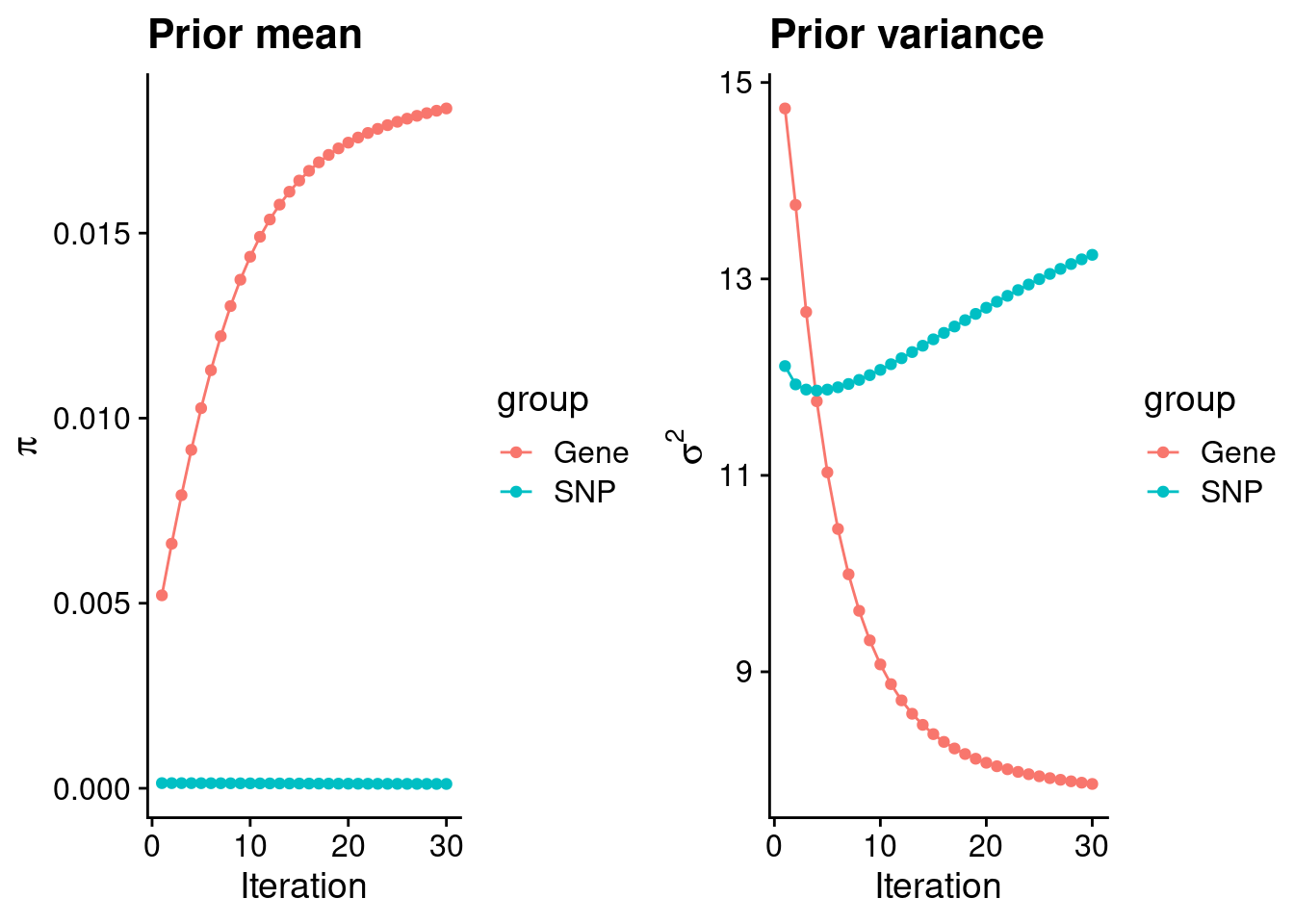
| Version | Author | Date |
|---|---|---|
| 3a7fbc1 | wesleycrouse | 2021-09-08 |
#estimated group prior
estimated_group_prior <- group_prior_rec[,ncol(group_prior_rec)]
names(estimated_group_prior) <- c("gene", "snp")
estimated_group_prior["snp"] <- estimated_group_prior["snp"]*thin #adjust parameter to account for thin argument
print(estimated_group_prior)
gene snp
0.0183686482 0.0001173307 #estimated group prior variance
estimated_group_prior_var <- group_prior_var_rec[,ncol(group_prior_var_rec)]
names(estimated_group_prior_var) <- c("gene", "snp")
print(estimated_group_prior_var) gene snp
7.858137 13.245400 #report sample size
print(sample_size)[1] 314916#report group size
group_size <- c(nrow(ctwas_gene_res), n_snps)
print(group_size)[1] 12810 8696600#estimated group PVE
estimated_group_pve <- estimated_group_prior_var*estimated_group_prior*group_size/sample_size #check PVE calculation
names(estimated_group_pve) <- c("gene", "snp")
print(estimated_group_pve) gene snp
0.005871529 0.042917199 #compare sum(PIP*mu2/sample_size) with above PVE calculation
c(sum(ctwas_gene_res$PVE),sum(ctwas_snp_res$PVE))[1] 0.0335362 0.2442329Genes with highest PIPs
#distribution of PIPs
hist(ctwas_gene_res$susie_pip, xlim=c(0,1), main="Distribution of Gene PIPs")
| Version | Author | Date |
|---|---|---|
| 3a7fbc1 | wesleycrouse | 2021-09-08 |
#genes with PIP>0.8 or 20 highest PIPs
head(ctwas_gene_res[order(-ctwas_gene_res$susie_pip),report_cols], max(sum(ctwas_gene_res$susie_pip>0.8), 20))
genename region_tag susie_pip mu2 PVE z
1230 CPNE3 8_62 0.993 27.52 8.7e-05 5.31
9162 USP47 11_9 0.989 31.59 9.9e-05 -5.37
13975 FBXO17 19_26 0.982 27.98 8.7e-05 5.23
11636 ELANE 19_2 0.965 20.66 6.3e-05 -4.38
4207 PPDPF 20_37 0.962 22.56 6.9e-05 -4.67
7232 NAT2 8_21 0.946 22.86 6.9e-05 -4.74
3645 CCND2 12_4 0.926 111.37 3.3e-04 -11.04
4035 ACVR1C 2_94 0.902 31.01 8.9e-05 -5.75
25 DBNDD1 16_54 0.864 19.98 5.5e-05 -4.47
4576 APOC1 19_31 0.864 18.87 5.2e-05 3.94
8942 WFDC13 20_28 0.864 21.31 5.9e-05 4.48
10806 SNN 16_13 0.861 19.35 5.3e-05 -4.18
677 BCAS1 20_32 0.820 19.73 5.1e-05 4.01
9614 TNFRSF10C 8_24 0.805 20.45 5.2e-05 4.03
11264 C15orf52 15_14 0.794 21.47 5.4e-05 4.53
5844 USP3 15_29 0.789 18.74 4.7e-05 4.09
6135 PRCC 1_77 0.787 23.59 5.9e-05 4.88
14031 RP11-105N14.1 2_126 0.784 20.88 5.2e-05 4.44
4811 FIGNL1 7_36 0.781 21.58 5.4e-05 -5.00
3080 NNT 5_28 0.777 19.38 4.8e-05 -4.04Genes with largest effect sizes
#plot PIP vs effect size
plot(ctwas_gene_res$susie_pip, ctwas_gene_res$mu2, xlab="PIP", ylab="mu^2", main="Gene PIPs vs Effect Size")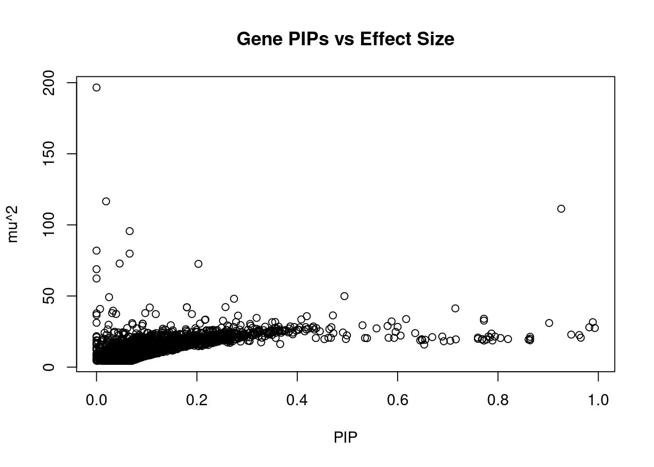
| Version | Author | Date |
|---|---|---|
| 3a7fbc1 | wesleycrouse | 2021-09-08 |
#genes with 20 largest effect sizes
head(ctwas_gene_res[order(-ctwas_gene_res$mu2),report_cols],20)
genename region_tag susie_pip mu2 PVE z
14585 LINC00506 3_57 0.000 196.59 0.0e+00 -1.09
6931 G6PC2 2_102 0.019 116.54 7.1e-06 -23.74
3645 CCND2 12_4 0.926 111.37 3.3e-04 -11.04
3273 NRBP1 2_16 0.066 95.63 2.0e-05 -10.35
2461 GCK 7_32 0.000 81.90 1.9e-10 13.60
3277 SNX17 2_16 0.066 79.79 1.7e-05 -9.16
3279 PPM1G 2_16 0.046 72.84 1.1e-05 -8.87
14565 LINC01126 2_27 0.203 72.60 4.7e-05 -8.98
590 CAMK2B 7_32 0.000 68.87 9.2e-08 5.10
6930 SPC25 2_102 0.000 62.33 2.3e-10 4.76
9611 PEAK1 15_36 0.494 49.91 7.8e-05 -7.25
3379 THADA 2_27 0.025 49.19 3.8e-06 7.95
6712 FADS1 11_34 0.274 48.06 4.2e-05 6.47
2811 MADD 11_29 0.257 42.20 3.4e-05 5.83
328 NR1H3 11_29 0.180 42.06 2.4e-05 7.38
5053 ACP2 11_29 0.180 42.06 2.4e-05 -7.38
8071 DNAJC5G 2_16 0.106 41.90 1.4e-05 5.92
11815 C2CD4A 15_28 0.715 41.29 9.4e-05 6.90
2463 YKT6 7_32 0.007 40.90 8.7e-07 11.82
4021 KBTBD4 11_29 0.033 39.65 4.2e-06 -7.05Genes with highest PVE
#genes with 20 highest pve
head(ctwas_gene_res[order(-ctwas_gene_res$PVE),report_cols],20)
genename region_tag susie_pip mu2 PVE z
3645 CCND2 12_4 0.926 111.37 3.3e-04 -11.04
9162 USP47 11_9 0.989 31.59 9.9e-05 -5.37
11815 C2CD4A 15_28 0.715 41.29 9.4e-05 6.90
4035 ACVR1C 2_94 0.902 31.01 8.9e-05 -5.75
1230 CPNE3 8_62 0.993 27.52 8.7e-05 5.31
13975 FBXO17 19_26 0.982 27.98 8.7e-05 5.23
3660 CTNNAL1 9_55 0.772 34.01 8.3e-05 -5.94
135 LUC7L 16_1 0.772 32.69 8.0e-05 7.44
9611 PEAK1 15_36 0.494 49.91 7.8e-05 -7.25
7232 NAT2 8_21 0.946 22.86 6.9e-05 -4.74
4207 PPDPF 20_37 0.962 22.56 6.9e-05 -4.67
12024 RNF5 6_26 0.617 33.79 6.6e-05 -6.52
11636 ELANE 19_2 0.965 20.66 6.3e-05 -4.38
7493 UBE2Z 17_28 0.588 32.14 6.0e-05 -5.77
6135 PRCC 1_77 0.787 23.59 5.9e-05 4.88
8942 WFDC13 20_28 0.864 21.31 5.9e-05 4.48
25 DBNDD1 16_54 0.864 19.98 5.5e-05 -4.47
5226 ABCB10 1_117 0.600 28.30 5.4e-05 5.41
2722 WFS1 4_7 0.471 36.35 5.4e-05 6.28
4811 FIGNL1 7_36 0.781 21.58 5.4e-05 -5.00Genes with largest z scores
#genes with 20 largest z scores
head(ctwas_gene_res[order(-abs(ctwas_gene_res$z)),report_cols],20)
genename region_tag susie_pip mu2 PVE z
6931 G6PC2 2_102 0.019 116.54 7.1e-06 -23.74
2461 GCK 7_32 0.000 81.90 1.9e-10 13.60
2463 YKT6 7_32 0.007 40.90 8.7e-07 11.82
3645 CCND2 12_4 0.926 111.37 3.3e-04 -11.04
3273 NRBP1 2_16 0.066 95.63 2.0e-05 -10.35
3277 SNX17 2_16 0.066 79.79 1.7e-05 -9.16
14565 LINC01126 2_27 0.203 72.60 4.7e-05 -8.98
3279 PPM1G 2_16 0.046 72.84 1.1e-05 -8.87
3379 THADA 2_27 0.025 49.19 3.8e-06 7.95
8825 FAM234A 16_1 0.419 35.82 4.8e-05 7.82
8019 EIF5A2 3_104 0.031 37.98 3.7e-06 7.76
135 LUC7L 16_1 0.772 32.69 8.0e-05 7.44
328 NR1H3 11_29 0.180 42.06 2.4e-05 7.38
5053 ACP2 11_29 0.180 42.06 2.4e-05 -7.38
9611 PEAK1 15_36 0.494 49.91 7.8e-05 -7.25
4021 KBTBD4 11_29 0.033 39.65 4.2e-06 -7.05
11815 C2CD4A 15_28 0.715 41.29 9.4e-05 6.90
1072 UBE2D4 7_32 0.000 37.80 5.3e-11 -6.85
9297 RBKS 2_16 0.097 37.98 1.2e-05 -6.54
12024 RNF5 6_26 0.617 33.79 6.6e-05 -6.52Comparing z scores and PIPs
#set nominal signifiance threshold for z scores
alpha <- 0.05

#bonferroni adjusted threshold for z scores
sig_thresh <- qnorm(1-(alpha/nrow(ctwas_gene_res)/2), lower=T)

#Q-Q plot for z scores
obs_z <- ctwas_gene_res$z[order(ctwas_gene_res$z)]
exp_z <- qnorm((1:nrow(ctwas_gene_res))/nrow(ctwas_gene_res))

plot(exp_z, obs_z, xlab="Expected z", ylab="Observed z", main="Gene z score Q-Q plot")
abline(a=0,b=1)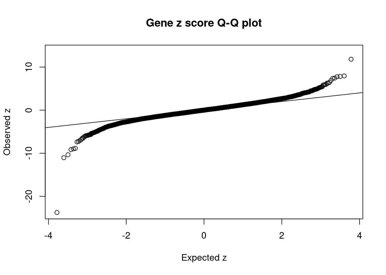
| Version | Author | Date |
|---|---|---|
| 3a7fbc1 | wesleycrouse | 2021-09-08 |
#plot z score vs PIP
plot(abs(ctwas_gene_res$z), ctwas_gene_res$susie_pip, xlab="abs(z)", ylab="PIP")
abline(v=sig_thresh, col="red", lty=2)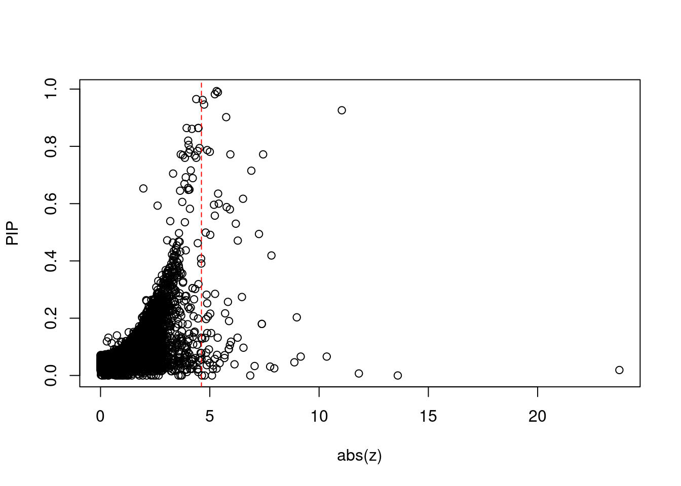
| Version | Author | Date |
|---|---|---|
| 3a7fbc1 | wesleycrouse | 2021-09-08 |
#proportion of significant z scores
mean(abs(ctwas_gene_res$z) > sig_thresh)
[1] 0.006010929#genes with most significant z scores
head(ctwas_gene_res[order(-abs(ctwas_gene_res$z)),report_cols],20) genename region_tag susie_pip mu2 PVE z
6931 G6PC2 2_102 0.019 116.54 7.1e-06 -23.74
2461 GCK 7_32 0.000 81.90 1.9e-10 13.60
2463 YKT6 7_32 0.007 40.90 8.7e-07 11.82
3645 CCND2 12_4 0.926 111.37 3.3e-04 -11.04
3273 NRBP1 2_16 0.066 95.63 2.0e-05 -10.35
3277 SNX17 2_16 0.066 79.79 1.7e-05 -9.16
14565 LINC01126 2_27 0.203 72.60 4.7e-05 -8.98
3279 PPM1G 2_16 0.046 72.84 1.1e-05 -8.87
3379 THADA 2_27 0.025 49.19 3.8e-06 7.95
8825 FAM234A 16_1 0.419 35.82 4.8e-05 7.82
8019 EIF5A2 3_104 0.031 37.98 3.7e-06 7.76
135 LUC7L 16_1 0.772 32.69 8.0e-05 7.44
328 NR1H3 11_29 0.180 42.06 2.4e-05 7.38
5053 ACP2 11_29 0.180 42.06 2.4e-05 -7.38
9611 PEAK1 15_36 0.494 49.91 7.8e-05 -7.25
4021 KBTBD4 11_29 0.033 39.65 4.2e-06 -7.05
11815 C2CD4A 15_28 0.715 41.29 9.4e-05 6.90
1072 UBE2D4 7_32 0.000 37.80 5.3e-11 -6.85
9297 RBKS 2_16 0.097 37.98 1.2e-05 -6.54
12024 RNF5 6_26 0.617 33.79 6.6e-05 -6.52Locus plots for genes and SNPs
ctwas_gene_res_sortz <- ctwas_gene_res[order(-abs(ctwas_gene_res$z)),]

n_plots <- 5
for (region_tag_plot in head(unique(ctwas_gene_res_sortz$region_tag), n_plots)){
  ctwas_res_region <-  ctwas_res[ctwas_res$region_tag==region_tag_plot,]
  start <- min(ctwas_res_region$pos)
  end <- max(ctwas_res_region$pos)

  ctwas_res_region <- ctwas_res_region[order(ctwas_res_region$pos),]
  ctwas_res_region_gene <- ctwas_res_region[ctwas_res_region$type=="gene",]
  ctwas_res_region_snp <- ctwas_res_region[ctwas_res_region$type=="SNP",]

  #region name
  print(paste0("Region: ", region_tag_plot))

  #table of genes in region
  print(ctwas_res_region_gene[,report_cols])

  par(mfrow=c(4,1))

  #gene z scores
  plot(ctwas_res_region_gene$pos, abs(ctwas_res_region_gene$z), xlab="Position", ylab="abs(gene_z)", xlim=c(start,end),
   ylim=c(0,max(sig_thresh, abs(ctwas_res_region_gene$z))),
   main=paste0("Region: ", region_tag_plot))
  abline(h=sig_thresh,col="red",lty=2)

  #significance threshold for SNPs
  alpha_snp <- 5*10^(-8)
  sig_thresh_snp <- qnorm(1-alpha_snp/2, lower=T)

  #snp z scores
  plot(ctwas_res_region_snp$pos, abs(ctwas_res_region_snp$z), xlab="Position", ylab="abs(snp_z)",xlim=c(start,end),
   ylim=c(0,max(sig_thresh_snp, max(abs(ctwas_res_region_snp$z)))))
  abline(h=sig_thresh_snp,col="purple",lty=2)

  #gene pips
  plot(ctwas_res_region_gene$pos, ctwas_res_region_gene$susie_pip, xlab="Position", ylab="Gene PIP", xlim=c(start,end), ylim=c(0,1))
  abline(h=0.8,col="blue",lty=2)

  #snp pips
  plot(ctwas_res_region_snp$pos, ctwas_res_region_snp$susie_pip, xlab="Position", ylab="SNP PIP", xlim=c(start,end), ylim=c(0,1))
  abline(h=0.8,col="blue",lty=2)
}
[1] "Region: 2_102"
genename region_tag susie_pip mu2 PVE z
7925 XIRP2 2_102 0.000 5.94 7.4e-12 -0.72
9457 CERS6 2_102 0.000 5.02 5.6e-12 -2.11
7922 NOSTRIN 2_102 0.000 36.57 4.1e-11 -2.31
6930 SPC25 2_102 0.000 62.33 2.3e-10 4.76
6931 G6PC2 2_102 0.019 116.54 7.1e-06 -23.74
920 ABCB11 2_102 0.000 18.90 1.9e-10 -1.01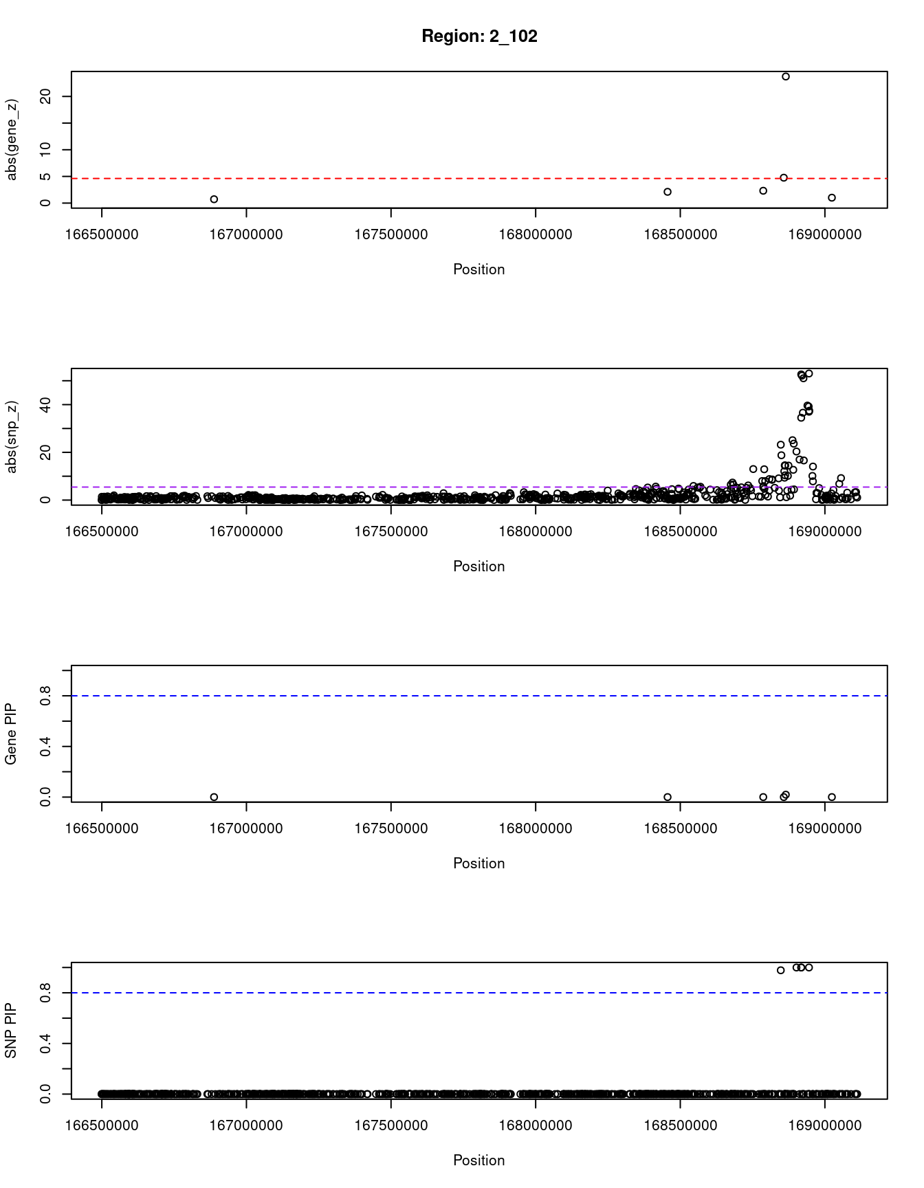
| Version | Author | Date |
|---|---|---|
| 3a7fbc1 | wesleycrouse | 2021-09-08 |
[1] "Region: 7_32"
        genename region_tag susie_pip   mu2     PVE     z
18         HECW1       7_32     0.000  6.92 1.1e-11  2.53
8238      STK17A       7_32     0.000  8.22 1.5e-11  0.69
2452        COA1       7_32     0.000 17.10 1.3e-10 -1.93
2453       BLVRA       7_32     0.000  5.56 7.9e-12 -1.22
636       MRPS24       7_32     0.000 11.92 4.7e-11  0.07
1072      UBE2D4       7_32     0.000 37.80 5.3e-11 -6.85
12678 AC004951.6       7_32     0.000  8.74 1.3e-11 -0.37
12901  LINC00957       7_32     0.000 16.03 4.6e-11  4.64
5305        DBNL       7_32     0.000 16.27 3.4e-11  2.66
3955        POLM       7_32     0.000  9.28 2.2e-11 -0.75
2458       AEBP1       7_32     0.000 21.02 3.0e-11  3.57
2461         GCK       7_32     0.000 81.90 1.9e-10 13.60
2463        YKT6       7_32     0.007 40.90 8.7e-07 11.82
590       CAMK2B       7_32     0.000 68.87 9.2e-08  5.10
266       NPC1L1       7_32     0.000 13.06 3.1e-11 -0.90
5303       DDX56       7_32     0.000 16.95 3.1e-11 -3.66
7444       TMED4       7_32     0.000 15.81 9.1e-11  1.43
2371        OGDH       7_32     0.000  9.38 1.9e-11  1.20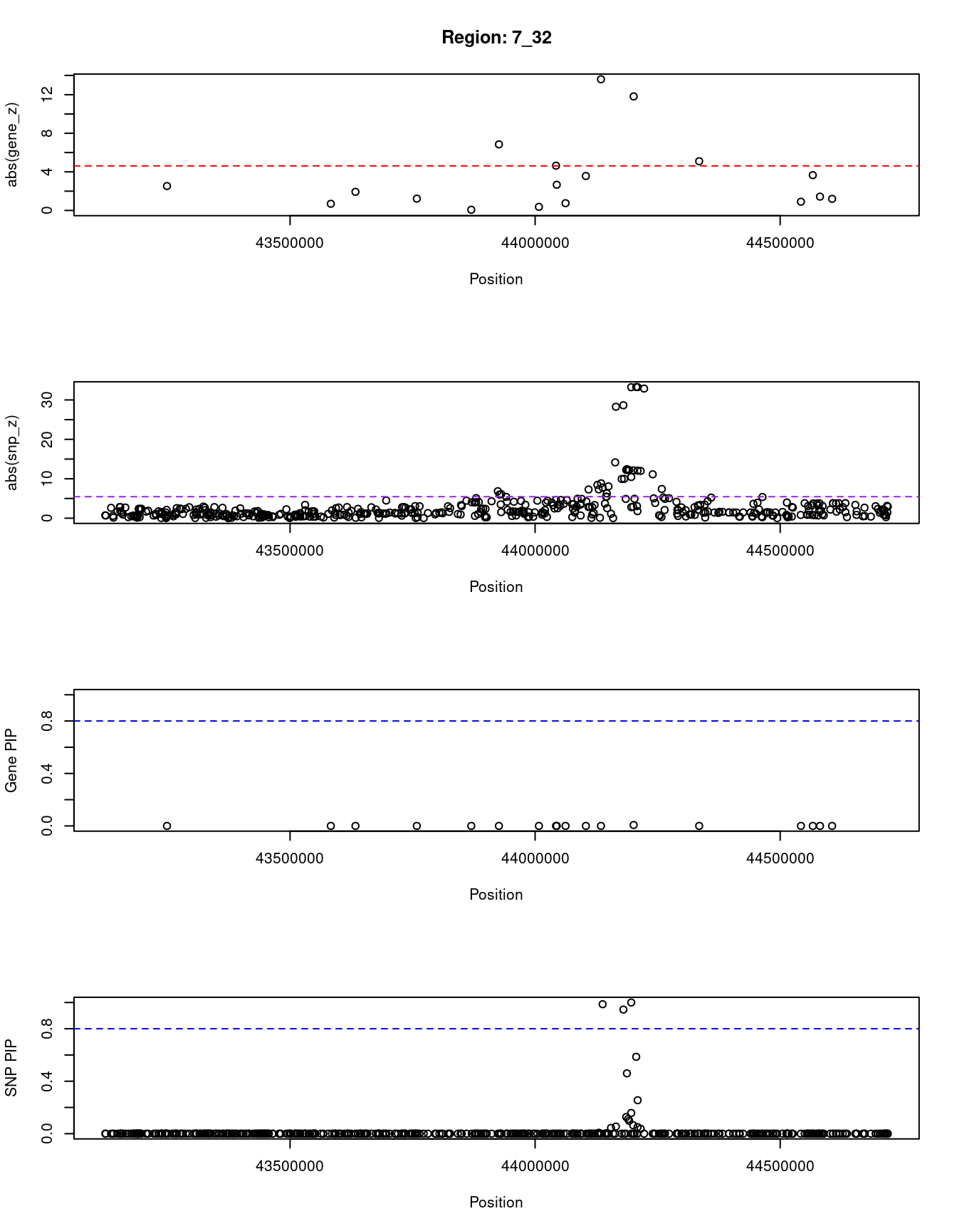
| Version | Author | Date |
|---|---|---|
| 3a7fbc1 | wesleycrouse | 2021-09-08 |
[1] "Region: 12_4"
     genename region_tag susie_pip    mu2     PVE      z
4564  CRACR2A       12_4     0.015   6.93 3.3e-07   1.01
2869   PARP11       12_4     0.013   5.07 2.1e-07   0.47
3645    CCND2       12_4     0.926 111.37 3.3e-04 -11.04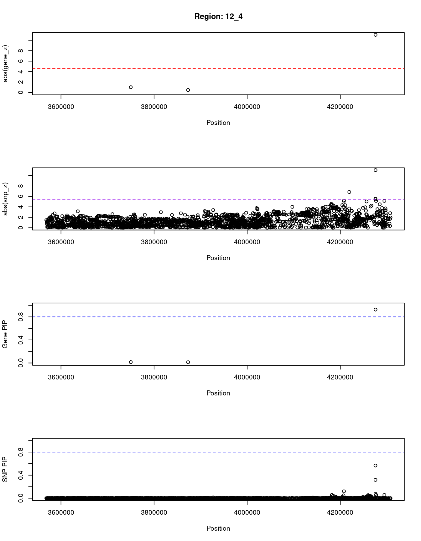
| Version | Author | Date |
|---|---|---|
| 3a7fbc1 | wesleycrouse | 2021-09-08 |
[1] "Region: 2_16"
       genename region_tag susie_pip   mu2     PVE      z
9315      KCNK3       2_16     0.037  5.49 6.5e-07   0.23
12312   SLC35F6       2_16     0.062 17.75 3.5e-06  -4.54
3267      CENPA       2_16     0.038  8.78 1.1e-06  -2.56
1209     MAPRE3       2_16     0.199 17.82 1.1e-05   4.46
5567    EMILIN1       2_16     0.045 10.09 1.5e-06   3.04
5552        KHK       2_16     0.054 14.33 2.4e-06   3.79
5550     CGREF1       2_16     0.035  6.54 7.2e-07   0.84
6260      ABHD1       2_16     0.035 10.56 1.2e-06   3.80
5562       PREB       2_16     0.045  9.13 1.3e-06   0.81
5568     ATRAID       2_16     0.039 19.19 2.4e-06   4.21
5563     SLC5A6       2_16     0.035 24.10 2.7e-06  -5.16
1210        CAD       2_16     0.035  4.65 5.1e-07   0.52
8071    DNAJC5G       2_16     0.106 41.90 1.4e-05   5.92
3271    SLC30A3       2_16     0.036 24.90 2.9e-06   4.86
8072        UCN       2_16     0.035  8.88 9.8e-07  -2.74
3277      SNX17       2_16     0.066 79.79 1.7e-05  -9.16
8073     ZNF513       2_16     0.035 13.98 1.6e-06  -3.39
3279      PPM1G       2_16     0.046 72.84 1.1e-05  -8.87
3273      NRBP1       2_16     0.066 95.63 2.0e-05 -10.35
7393    KRTCAP3       2_16     0.047 15.00 2.2e-06  -3.56
11814      GPN1       2_16     0.068  8.82 1.9e-06   0.32
9963    CCDC121       2_16     0.066  8.61 1.8e-06   0.35
8074   SLC4A1AP       2_16     0.036 12.29 1.4e-06   2.27
12161 LINC01460       2_16     0.058 24.08 4.4e-06  -5.23
7398        BRE       2_16     0.064 17.49 3.6e-06  -3.59
9297       RBKS       2_16     0.097 37.98 1.2e-05  -6.54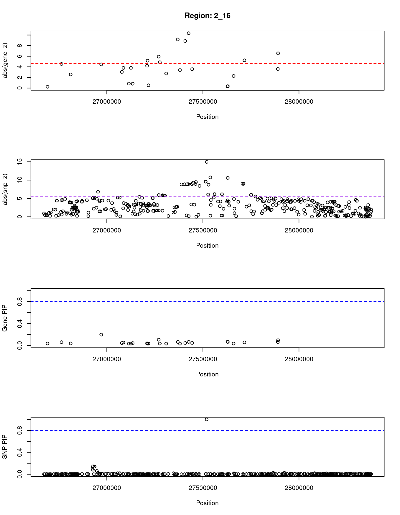
| Version | Author | Date |
|---|---|---|
| 3a7fbc1 | wesleycrouse | 2021-09-08 |
[1] "Region: 2_27"
        genename region_tag susie_pip   mu2     PVE     z
14565  LINC01126       2_27     0.203 72.60 4.7e-05 -8.98
3379       THADA       2_27     0.025 49.19 3.8e-06  7.95
12512 C1GALT1C1L       2_27     0.034  7.18 7.8e-07  0.80
6962     PLEKHH2       2_27     0.031  6.66 6.6e-07  0.60
5556    DYNC2LI1       2_27     0.060 14.04 2.7e-06 -2.02
6249       ABCG8       2_27     0.105 20.68 6.9e-06  3.16
5564       ABCG5       2_27     0.045 10.14 1.4e-06  1.21
5570      LRPPRC       2_27     0.044 10.83 1.5e-06 -1.66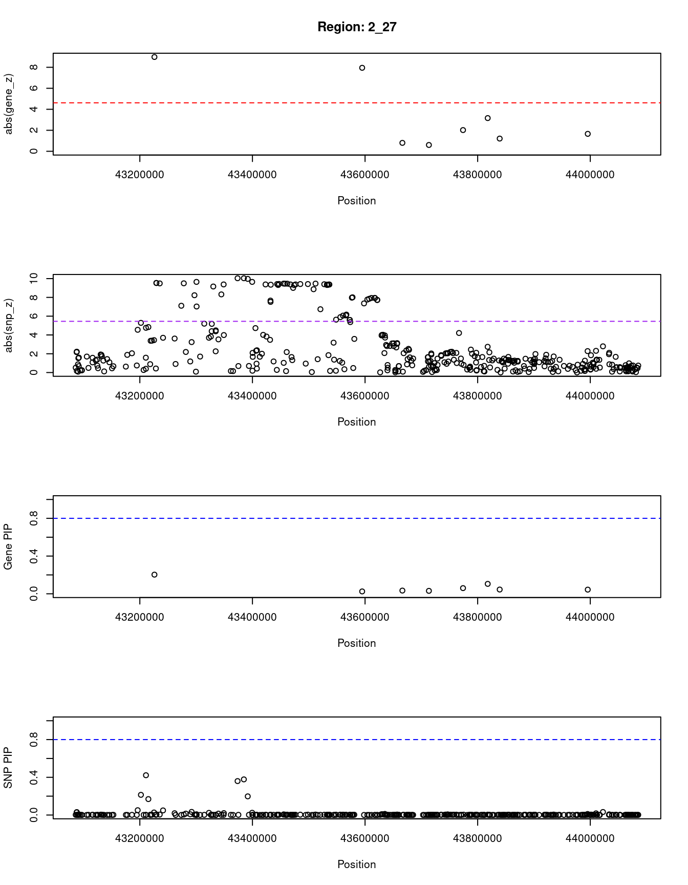
| Version | Author | Date |
|---|---|---|
| 3a7fbc1 | wesleycrouse | 2021-09-08 |
SNPs with highest PIPs
#snps with PIP>0.8 or 20 highest PIPs
head(ctwas_snp_res[order(-ctwas_snp_res$susie_pip),report_cols_snps],
max(sum(ctwas_snp_res$susie_pip>0.8), 20))
id region_tag susie_pip mu2 PVE z
54257 rs79687284 1_108 1.000 113.35 3.6e-04 -12.08
75329 rs780093 2_16 1.000 191.48 6.1e-04 -14.95
81655 rs2121564 2_28 1.000 61.61 2.0e-04 -8.01
114233 rs12692596 2_96 1.000 46.76 1.5e-04 -7.24
116525 rs11396827 2_102 1.000 211.97 6.7e-04 -20.35
116527 rs71397673 2_102 1.000 482.06 1.5e-03 -34.50
116528 rs537183 2_102 1.000 878.67 2.8e-03 -52.66
116535 rs853789 2_102 1.000 906.59 2.9e-03 -53.04
165897 rs148685409 3_57 1.000 1085.70 3.4e-03 2.99
176009 rs72964564 3_76 1.000 246.70 7.8e-04 16.88
196056 rs4234603 3_115 1.000 40.78 1.3e-04 -5.05
322901 rs76623841 6_7 1.000 59.67 1.9e-04 6.80
385601 rs10225316 7_15 1.000 46.25 1.5e-04 -7.51
395838 rs138917529 7_32 1.000 79.53 2.5e-04 10.45
435615 rs7012814 8_12 1.000 63.67 2.0e-04 9.18
529384 rs61856594 10_33 1.000 38.90 1.2e-04 6.23
549195 rs12244851 10_70 1.000 302.25 9.6e-04 -16.46
557501 rs3842727 11_3 1.000 104.08 3.3e-04 8.57
645018 rs576674 13_10 1.000 107.45 3.4e-04 10.82
694011 rs35889227 14_46 1.000 118.49 3.8e-04 11.34
287441 rs12189028 5_45 0.999 35.54 1.1e-04 5.08
477509 rs10758593 9_4 0.999 72.89 2.3e-04 -8.64
907071 rs2168101 11_6 0.999 69.37 2.2e-04 8.60
54266 rs3754140 1_108 0.998 59.12 1.9e-04 10.01
235112 rs11728350 4_69 0.998 43.60 1.4e-04 -6.68
511130 rs115478735 9_70 0.997 84.00 2.7e-04 -9.52
322920 rs55792466 6_7 0.994 100.94 3.2e-04 9.67
484749 rs572168822 9_16 0.994 42.02 1.3e-04 6.61
659663 rs1327315 13_40 0.994 36.53 1.2e-04 7.02
636136 rs4765221 12_76 0.990 34.47 1.1e-04 -5.80
809860 rs34783010 19_32 0.990 32.48 1.0e-04 6.40
557506 rs10743152 11_3 0.989 42.45 1.3e-04 -1.91
395818 rs17769733 7_32 0.987 140.84 4.4e-04 7.76
548647 rs11195508 10_70 0.987 61.59 1.9e-04 10.76
116507 rs11676084 2_102 0.978 129.32 4.0e-04 23.20
484744 rs1333045 9_16 0.977 41.79 1.3e-04 -6.62
412817 rs4729755 7_63 0.974 26.75 8.3e-05 -4.96
705010 rs12912777 15_13 0.972 26.19 8.1e-05 -3.77
755487 rs28489441 17_15 0.972 32.37 1.0e-04 5.83
190899 rs10653660 3_104 0.971 358.85 1.1e-03 23.54
755 rs60330317 1_2 0.970 37.65 1.2e-04 6.18
475467 rs4977218 8_94 0.970 30.69 9.4e-05 5.34
643328 rs60353775 13_7 0.970 84.44 2.6e-04 -9.78
627635 rs6538805 12_58 0.969 32.51 1.0e-04 6.74
466214 rs4433184 8_78 0.968 55.47 1.7e-04 -4.78
174043 rs9875598 3_73 0.963 27.81 8.5e-05 5.10
671591 rs80081165 13_62 0.958 25.98 7.9e-05 -4.82
797735 rs10410896 19_5 0.951 28.01 8.5e-05 -5.04
831061 rs6026545 20_34 0.947 34.47 1.0e-04 -5.72
395830 rs10259649 7_32 0.946 400.33 1.2e-03 -28.65
701487 rs35767992 15_4 0.946 24.90 7.5e-05 -4.72
571136 rs7111517 11_28 0.941 40.02 1.2e-04 6.64
512420 rs28624681 9_73 0.937 51.58 1.5e-04 -7.55
570939 rs117396352 11_28 0.929 27.67 8.2e-05 -4.93
756996 rs543720569 17_18 0.929 45.45 1.3e-04 7.03
712417 rs11637069 15_29 0.924 29.01 8.5e-05 -5.00
454310 rs10957704 8_54 0.920 25.06 7.3e-05 -4.68
575070 rs7941126 11_36 0.909 31.74 9.2e-05 5.63
571959 rs182512331 11_31 0.902 28.13 8.1e-05 5.05
168814 rs62276527 3_63 0.897 33.88 9.6e-05 -5.85
561389 rs117720468 11_11 0.894 45.27 1.3e-04 -6.82
336612 rs62396405 6_30 0.892 26.09 7.4e-05 4.78
639168 rs1882297 12_82 0.886 39.86 1.1e-04 -6.47
365610 rs112388031 6_87 0.882 25.27 7.1e-05 4.65
287502 rs6887019 5_45 0.881 27.15 7.6e-05 -5.23
541735 rs11202472 10_56 0.873 32.03 8.9e-05 4.88
359132 rs118126621 6_73 0.872 25.87 7.2e-05 -4.67
154326 rs3172494 3_34 0.864 26.99 7.4e-05 5.09
571541 rs139913257 11_30 0.864 32.33 8.9e-05 5.63
795104 rs41404946 18_44 0.855 25.13 6.8e-05 -4.56
34659 rs893230 1_72 0.846 40.72 1.1e-04 7.56
19026 rs6699568 1_42 0.836 27.89 7.4e-05 -5.02
257247 rs62332172 4_113 0.833 25.19 6.7e-05 -4.54
398174 rs11763778 7_36 0.825 41.96 1.1e-04 7.61
660014 rs79317015 13_40 0.812 25.51 6.6e-05 -4.40
577100 rs11603349 11_41 0.811 45.92 1.2e-04 6.78
195596 rs73185688 3_114 0.806 25.78 6.6e-05 -4.69
605450 rs12582270 12_17 0.806 26.39 6.8e-05 4.72SNPs with largest effect sizes
#plot PIP vs effect size
plot(ctwas_snp_res$susie_pip, ctwas_snp_res$mu2, xlab="PIP", ylab="mu^2", main="SNP PIPs vs Effect Size")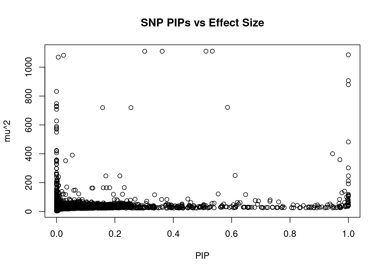
| Version | Author | Date |
|---|---|---|
| 3a7fbc1 | wesleycrouse | 2021-09-08 |
#SNPs with 50 largest effect sizes
head(ctwas_snp_res[order(-ctwas_snp_res$mu2),report_cols_snps],50)
id region_tag susie_pip mu2 PVE z
165900 rs7619398 3_57 0.534 1111.07 1.9e-03 3.08
165899 rs1436648 3_57 0.512 1110.80 1.8e-03 3.09
165901 rs2256473 3_57 0.362 1110.33 1.3e-03 3.06
165898 rs2575789 3_57 0.302 1110.24 1.1e-03 3.06
165897 rs148685409 3_57 1.000 1085.70 3.4e-03 2.99
165907 rs7620974 3_57 0.024 1082.35 8.2e-05 -2.95
165908 rs2575752 3_57 0.006 1069.54 2.0e-05 3.11
116535 rs853789 2_102 1.000 906.59 2.9e-03 -53.04
116528 rs537183 2_102 1.000 878.67 2.8e-03 -52.66
116529 rs518598 2_102 0.000 831.75 3.8e-08 -52.13
165910 rs2575762 3_57 0.000 747.27 0.0e+00 3.39
165922 rs9284813 3_57 0.000 730.46 0.0e+00 -3.52
116531 rs485094 2_102 0.000 726.68 1.2e-10 -51.04
395843 rs917793 7_32 0.586 721.59 1.3e-03 -33.28
395847 rs2908282 7_32 0.255 719.52 5.8e-04 -33.26
395837 rs4607517 7_32 0.158 719.46 3.6e-04 -33.23
395849 rs732360 7_32 0.000 708.00 8.0e-07 -32.89
165927 rs6775215 3_57 0.000 627.62 0.0e+00 -3.37
165925 rs12631713 3_57 0.000 588.77 0.0e+00 -3.29
116533 rs2544360 2_102 0.000 580.12 1.7e-10 -39.60
165919 rs6791960 3_57 0.000 570.74 0.0e+00 -3.17
165912 rs1036446 3_57 0.000 570.38 0.0e+00 3.12
116534 rs853791 2_102 0.000 549.87 8.8e-11 -39.21
116527 rs71397673 2_102 1.000 482.06 1.5e-03 -34.50
116530 rs579275 2_102 0.000 423.03 2.9e-11 -36.60
116537 rs853785 2_102 0.000 419.12 3.2e-11 -37.45
116536 rs860510 2_102 0.000 406.57 3.3e-11 -37.03
395830 rs10259649 7_32 0.946 400.33 1.2e-03 -28.65
395828 rs2908294 7_32 0.054 390.64 6.7e-05 -28.27
190899 rs10653660 3_104 0.971 358.85 1.1e-03 23.54
165913 rs78718649 3_57 0.000 358.13 0.0e+00 -1.33
165914 rs116802846 3_57 0.000 357.83 0.0e+00 -1.32
165915 rs199827403 3_57 0.000 357.39 0.0e+00 -1.32
165917 rs143745027 3_57 0.000 354.23 0.0e+00 -1.41
190909 rs8192675 3_104 0.031 351.51 3.4e-05 23.31
165909 rs2660761 3_57 0.000 350.36 0.0e+00 3.35
165920 rs7649216 3_57 0.000 343.56 0.0e+00 -3.61
165928 rs17181219 3_57 0.000 328.83 0.0e+00 -3.43
165943 rs9858014 3_57 0.000 328.78 0.0e+00 -1.31
165960 rs1002765 3_57 0.000 328.73 0.0e+00 -1.99
549195 rs12244851 10_70 1.000 302.25 9.6e-04 -16.46
165932 rs6805536 3_57 0.000 298.41 0.0e+00 -3.05
165930 rs6783908 3_57 0.000 298.36 0.0e+00 -3.04
165933 rs1844099 3_57 0.000 298.23 0.0e+00 -3.05
395827 rs758989 7_32 0.000 267.44 6.8e-09 -14.16
165945 rs75004821 3_57 0.000 259.17 0.0e+00 -1.54
165946 rs73846673 3_57 0.000 258.08 0.0e+00 -1.54
165948 rs116525622 3_57 0.000 257.36 0.0e+00 -1.52
165949 rs75023402 3_57 0.000 257.35 0.0e+00 -1.53
549203 rs12260037 10_70 0.000 255.59 4.7e-10 -17.19SNPs with highest PVE
#SNPs with 50 highest pve
head(ctwas_snp_res[order(-ctwas_snp_res$PVE),report_cols_snps],50)
id region_tag susie_pip mu2 PVE z
165897 rs148685409 3_57 1.000 1085.70 0.00340 2.99
116535 rs853789 2_102 1.000 906.59 0.00290 -53.04
116528 rs537183 2_102 1.000 878.67 0.00280 -52.66
165900 rs7619398 3_57 0.534 1111.07 0.00190 3.08
165899 rs1436648 3_57 0.512 1110.80 0.00180 3.09
116527 rs71397673 2_102 1.000 482.06 0.00150 -34.50
165901 rs2256473 3_57 0.362 1110.33 0.00130 3.06
395843 rs917793 7_32 0.586 721.59 0.00130 -33.28
395830 rs10259649 7_32 0.946 400.33 0.00120 -28.65
165898 rs2575789 3_57 0.302 1110.24 0.00110 3.06
190899 rs10653660 3_104 0.971 358.85 0.00110 23.54
549195 rs12244851 10_70 1.000 302.25 0.00096 -16.46
176009 rs72964564 3_76 1.000 246.70 0.00078 16.88
116525 rs11396827 2_102 1.000 211.97 0.00067 -20.35
75329 rs780093 2_16 1.000 191.48 0.00061 -14.95
395847 rs2908282 7_32 0.255 719.52 0.00058 -33.26
385661 rs1974619 7_15 0.612 249.26 0.00048 -16.89
395818 rs17769733 7_32 0.987 140.84 0.00044 7.76
116507 rs11676084 2_102 0.978 129.32 0.00040 23.20
694011 rs35889227 14_46 1.000 118.49 0.00038 11.34
54257 rs79687284 1_108 1.000 113.35 0.00036 -12.08
395837 rs4607517 7_32 0.158 719.46 0.00036 -33.23
645018 rs576674 13_10 1.000 107.45 0.00034 10.82
557501 rs3842727 11_3 1.000 104.08 0.00033 8.57
322920 rs55792466 6_7 0.994 100.94 0.00032 9.67
511130 rs115478735 9_70 0.997 84.00 0.00027 -9.52
643328 rs60353775 13_7 0.970 84.44 0.00026 -9.78
395838 rs138917529 7_32 1.000 79.53 0.00025 10.45
919509 rs11039165 11_29 0.648 116.99 0.00024 11.82
477509 rs10758593 9_4 0.999 72.89 0.00023 -8.64
907071 rs2168101 11_6 0.999 69.37 0.00022 8.60
292705 rs17085655 5_56 0.554 121.46 0.00021 11.48
81655 rs2121564 2_28 1.000 61.61 0.00020 -8.01
435615 rs7012814 8_12 1.000 63.67 0.00020 9.18
54266 rs3754140 1_108 0.998 59.12 0.00019 10.01
322901 rs76623841 6_7 1.000 59.67 0.00019 6.80
548647 rs11195508 10_70 0.987 61.59 0.00019 10.76
549189 rs117764423 10_70 0.732 80.43 0.00019 5.24
385659 rs10228796 7_15 0.217 246.79 0.00017 -16.82
466214 rs4433184 8_78 0.968 55.47 0.00017 -4.78
261331 rs12499544 4_119 0.731 70.23 0.00016 8.39
327512 rs2206734 6_15 0.761 66.38 0.00016 -8.26
466238 rs28529793 8_78 0.692 72.86 0.00016 6.80
822756 rs111405491 20_16 0.681 76.06 0.00016 8.97
114233 rs12692596 2_96 1.000 46.76 0.00015 -7.24
385601 rs10225316 7_15 1.000 46.25 0.00015 -7.51
512420 rs28624681 9_73 0.937 51.58 0.00015 -7.55
235112 rs11728350 4_69 0.998 43.60 0.00014 -6.68
196056 rs4234603 3_115 1.000 40.78 0.00013 -5.05
385660 rs2191349 7_15 0.169 246.29 0.00013 -16.80SNPs with largest z scores
#SNPs with 50 largest z scores
head(ctwas_snp_res[order(-abs(ctwas_snp_res$z)),report_cols_snps],50)
id region_tag susie_pip mu2 PVE z
116535 rs853789 2_102 1.000 906.59 2.9e-03 -53.04
116528 rs537183 2_102 1.000 878.67 2.8e-03 -52.66
116529 rs518598 2_102 0.000 831.75 3.8e-08 -52.13
116531 rs485094 2_102 0.000 726.68 1.2e-10 -51.04
116533 rs2544360 2_102 0.000 580.12 1.7e-10 -39.60
116534 rs853791 2_102 0.000 549.87 8.8e-11 -39.21
116537 rs853785 2_102 0.000 419.12 3.2e-11 -37.45
116536 rs860510 2_102 0.000 406.57 3.3e-11 -37.03
116530 rs579275 2_102 0.000 423.03 2.9e-11 -36.60
116527 rs71397673 2_102 1.000 482.06 1.5e-03 -34.50
395843 rs917793 7_32 0.586 721.59 1.3e-03 -33.28
395847 rs2908282 7_32 0.255 719.52 5.8e-04 -33.26
395837 rs4607517 7_32 0.158 719.46 3.6e-04 -33.23
395849 rs732360 7_32 0.000 708.00 8.0e-07 -32.89
395830 rs10259649 7_32 0.946 400.33 1.2e-03 -28.65
395828 rs2908294 7_32 0.054 390.64 6.7e-05 -28.27
116521 rs62176784 2_102 0.001 136.37 3.5e-07 25.09
116523 rs549410 2_102 0.000 186.76 2.6e-08 23.64
190899 rs10653660 3_104 0.971 358.85 1.1e-03 23.54
190909 rs8192675 3_104 0.031 351.51 3.4e-05 23.31
116507 rs11676084 2_102 0.978 129.32 4.0e-04 23.20
116525 rs11396827 2_102 1.000 211.97 6.7e-04 -20.35
116508 rs2140046 2_102 0.000 66.87 4.2e-09 18.78
190907 rs11920090 3_104 0.232 165.52 1.2e-04 18.33
190893 rs12492910 3_104 0.182 164.56 9.5e-05 18.32
190906 rs11923694 3_104 0.160 164.09 8.3e-05 18.31
190896 rs12496506 3_104 0.171 164.17 8.9e-05 18.30
190910 rs11928798 3_104 0.121 162.56 6.2e-05 18.26
190911 rs6785803 3_104 0.124 162.55 6.4e-05 18.25
190886 rs56351320 3_104 0.001 219.35 8.3e-07 17.54
190871 rs6792607 3_104 0.003 206.64 2.3e-06 17.19
549203 rs12260037 10_70 0.000 255.59 4.7e-10 -17.19
116526 rs13430620 2_102 0.000 91.03 1.1e-10 16.98
385661 rs1974619 7_15 0.612 249.26 4.8e-04 -16.89
176009 rs72964564 3_76 1.000 246.70 7.8e-04 16.88
385659 rs10228796 7_15 0.217 246.79 1.7e-04 -16.82
385660 rs2191349 7_15 0.169 246.29 1.3e-04 -16.80
116532 rs114932341 2_102 0.000 187.18 4.8e-10 -16.61
385662 rs188745922 7_15 0.007 240.15 5.7e-06 -16.59
549195 rs12244851 10_70 1.000 302.25 9.6e-04 -16.46
190863 rs11919048 3_104 0.018 139.06 7.9e-06 16.13
176007 rs34642857 3_76 0.003 224.87 2.1e-06 16.11
190878 rs79560566 3_104 0.001 131.23 3.6e-07 15.48
385657 rs6461153 7_15 0.001 212.60 9.0e-07 -15.42
385656 rs10266209 7_15 0.001 212.23 8.9e-07 -15.41
385655 rs10249299 7_15 0.002 212.31 1.4e-06 15.31
75329 rs780093 2_16 1.000 191.48 6.1e-04 -14.95
190901 rs143791579 3_104 0.001 100.18 3.0e-07 14.91
385650 rs4721398 7_15 0.001 195.58 7.6e-07 14.88
190894 rs73167792 3_104 0.001 97.26 3.2e-07 14.81Gene set enrichment for genes with PIP>0.8
#GO enrichment analysis
library(enrichR)
Welcome to enrichR
Checking connection ... Enrichr ... Connection is Live!
FlyEnrichr ... Connection is available!
WormEnrichr ... Connection is available!
YeastEnrichr ... Connection is available!
FishEnrichr ... Connection is available!dbs <- c("GO_Biological_Process_2021", "GO_Cellular_Component_2021", "GO_Molecular_Function_2021")
genes <- ctwas_gene_res$genename[ctwas_gene_res$susie_pip>0.8]
#number of genes for gene set enrichment
length(genes)[1] 14if (length(genes)>0){
GO_enrichment <- enrichr(genes, dbs)
for (db in dbs){
print(db)
df <- GO_enrichment[[db]]
df <- df[df$Adjusted.P.value<0.05,c("Term", "Overlap", "Adjusted.P.value", "Genes")]
print(df)
}
#DisGeNET enrichment
# devtools::install_bitbucket("ibi_group/disgenet2r")
library(disgenet2r)
disgenet_api_key <- get_disgenet_api_key(
email = "wesleycrouse@gmail.com",
password = "uchicago1" )
Sys.setenv(DISGENET_API_KEY= disgenet_api_key)
res_enrich <-disease_enrichment(entities=genes, vocabulary = "HGNC",
database = "CURATED" )
df <- res_enrich@qresult[1:10, c("Description", "FDR", "Ratio", "BgRatio")]
print(df)
#WebGestalt enrichment
library(WebGestaltR)
background <- ctwas_gene_res$genename
#listGeneSet()
databases <- c("pathway_KEGG", "disease_GLAD4U", "disease_OMIM")
enrichResult <- WebGestaltR(enrichMethod="ORA", organism="hsapiens",
interestGene=genes, referenceGene=background,
enrichDatabase=databases, interestGeneType="genesymbol",
referenceGeneType="genesymbol", isOutput=F)
print(enrichResult[,c("description", "size", "overlap", "FDR", "database", "userId")])
}Uploading data to Enrichr... Done.
Querying GO_Biological_Process_2021... Done.
Querying GO_Cellular_Component_2021... Done.
Querying GO_Molecular_Function_2021... Done.
Parsing results... Done.
[1] "GO_Biological_Process_2021"
[1] Term Overlap Adjusted.P.value Genes
<0 rows> (or 0-length row.names)
[1] "GO_Cellular_Component_2021"
Term Overlap
1 serine/threonine protein kinase complex (GO:1902554) 2/37
2 SCF ubiquitin ligase complex (GO:0019005) 2/58
3 activin receptor complex (GO:0048179) 1/7
4 azurophil granule (GO:0042582) 2/155
5 cullin-RING ubiquitin ligase complex (GO:0031461) 2/157
6 chylomicron (GO:0042627) 1/10
7 triglyceride-rich plasma lipoprotein particle (GO:0034385) 1/15
8 very-low-density lipoprotein particle (GO:0034361) 1/15
9 high-density lipoprotein particle (GO:0034364) 1/19
Adjusted.P.value Genes
1 0.008367022 ACVR1C;CCND2
2 0.010296634 USP47;FBXO17
3 0.029329321 ACVR1C
4 0.029329321 CPNE3;ELANE
5 0.029329321 USP47;FBXO17
6 0.032570877 APOC1
7 0.036582843 APOC1
8 0.036582843 APOC1
9 0.041136151 APOC1
[1] "GO_Molecular_Function_2021"
Term
1 activin receptor activity, type I (GO:0016361)
2 phosphatidylcholine-sterol O-acyltransferase activator activity (GO:0060228)
3 activin-activated receptor activity (GO:0017002)
4 phospholipase inhibitor activity (GO:0004859)
5 lipase inhibitor activity (GO:0055102)
Overlap Adjusted.P.value Genes
1 1/5 0.04327274 ACVR1C
2 1/6 0.04327274 APOC1
3 1/9 0.04327274 ACVR1C
4 1/10 0.04327274 APOC1
5 1/10 0.04327274 APOC1FBXO17 gene(s) from the input list not found in DisGeNET CURATEDPPDPF gene(s) from the input list not found in DisGeNET CURATEDSNN gene(s) from the input list not found in DisGeNET CURATEDWFDC13 gene(s) from the input list not found in DisGeNET CURATEDUSP47 gene(s) from the input list not found in DisGeNET CURATEDDBNDD1 gene(s) from the input list not found in DisGeNET CURATED Description
36 Prostatic Neoplasms
48 Cyclic neutropenia
59 Malignant neoplasm of prostate
94 Cyclic Hematopoesis
98 MEGALENCEPHALY-POLYMICROGYRIA-POLYDACTYLY-HYDROCEPHALUS SYNDROME 3
47 POLYDACTYLY, POSTAXIAL
78 Perisylvian syndrome
79 Neutropenia, Severe Congenital, Autosomal Dominant 1
80 Megalanecephaly Polymicrogyria-Polydactyly Hydrocephalus Syndrome
81 POSTAXIAL POLYDACTYLY, TYPE B
FDR Ratio BgRatio
36 0.01927702 4/8 616/9703
48 0.01927702 1/8 1/9703
59 0.01927702 4/8 616/9703
94 0.01927702 1/8 1/9703
98 0.01927702 1/8 1/9703
47 0.02661120 1/8 4/9703
78 0.02661120 1/8 4/9703
79 0.02661120 1/8 4/9703
80 0.02661120 1/8 4/9703
81 0.02661120 1/8 3/9703******************************************
* *
* Welcome to WebGestaltR ! *
* *
******************************************Loading the functional categories...
Loading the ID list...
Loading the reference list...
Performing the enrichment analysis...Warning in oraEnrichment(interestGeneList, referenceGeneList, geneSet,
minNum = minNum, : No significant gene set is identified based on FDR 0.05!NULLSensitivity, specificity and precision for silver standard genes
library("readxl")

known_annotations <- read_xlsx("data/summary_known_genes_annotations.xlsx", sheet="Glucose")
known_annotations <- unique(known_annotations$`Gene Symbol`)

unrelated_genes <- ctwas_gene_res$genename[!(ctwas_gene_res$genename %in% known_annotations)]

#number of genes in known annotations
print(length(known_annotations))
[1] 87#number of genes in known annotations with imputed expression
print(sum(known_annotations %in% ctwas_gene_res$genename))[1] 41#assign ctwas, TWAS, and bystander genes
ctwas_genes <- ctwas_gene_res$genename[ctwas_gene_res$susie_pip>0.8]
twas_genes <- ctwas_gene_res$genename[abs(ctwas_gene_res$z)>sig_thresh]
novel_genes <- ctwas_genes[!(ctwas_genes %in% twas_genes)]
#significance threshold for TWAS
print(sig_thresh)[1] 4.616471#number of ctwas genes
length(ctwas_genes)[1] 14#number of TWAS genes
length(twas_genes)[1] 77#show novel genes (ctwas genes with not in TWAS genes)
ctwas_gene_res[ctwas_gene_res$genename %in% novel_genes,report_cols] genename region_tag susie_pip mu2 PVE z
9614 TNFRSF10C 8_24 0.805 20.45 5.2e-05 4.03
10806 SNN 16_13 0.861 19.35 5.3e-05 -4.18
25 DBNDD1 16_54 0.864 19.98 5.5e-05 -4.47
11636 ELANE 19_2 0.965 20.66 6.3e-05 -4.38
4576 APOC1 19_31 0.864 18.87 5.2e-05 3.94
8942 WFDC13 20_28 0.864 21.31 5.9e-05 4.48
677 BCAS1 20_32 0.820 19.73 5.1e-05 4.01#sensitivity / recall
sensitivity <- rep(NA,2)
names(sensitivity) <- c("ctwas", "TWAS")
sensitivity["ctwas"] <- sum(ctwas_genes %in% known_annotations)/length(known_annotations)
sensitivity["TWAS"] <- sum(twas_genes %in% known_annotations)/length(known_annotations)
sensitivity ctwas TWAS
0.00000000 0.03448276 #specificity
specificity <- rep(NA,2)
names(specificity) <- c("ctwas", "TWAS")
specificity["ctwas"] <- sum(!(unrelated_genes %in% ctwas_genes))/length(unrelated_genes)
specificity["TWAS"] <- sum(!(unrelated_genes %in% twas_genes))/length(unrelated_genes)
specificity ctwas TWAS
0.9989036 0.9942047 #precision / PPV
precision <- rep(NA,2)
names(precision) <- c("ctwas", "TWAS")
precision["ctwas"] <- sum(ctwas_genes %in% known_annotations)/length(ctwas_genes)
precision["TWAS"] <- sum(twas_genes %in% known_annotations)/length(twas_genes)
precision ctwas TWAS
0.00000000 0.03896104 #ROC curves
pip_range <- (0:1000)/1000
sensitivity <- rep(NA, length(pip_range))
specificity <- rep(NA, length(pip_range))
for (index in 1:length(pip_range)){
pip <- pip_range[index]
ctwas_genes <- ctwas_gene_res$genename[ctwas_gene_res$susie_pip>=pip]
sensitivity[index] <- sum(ctwas_genes %in% known_annotations)/length(known_annotations)
specificity[index] <- sum(!(unrelated_genes %in% ctwas_genes))/length(unrelated_genes)
}
plot(1-specificity, sensitivity, type="l", xlim=c(0,1), ylim=c(0,1))
sig_thresh_range <- seq(from=0, to=max(abs(ctwas_gene_res$z)), length.out=length(pip_range))
for (index in 1:length(sig_thresh_range)){
sig_thresh_plot <- sig_thresh_range[index]
twas_genes <- ctwas_gene_res$genename[abs(ctwas_gene_res$z)>=sig_thresh_plot]
sensitivity[index] <- sum(twas_genes %in% known_annotations)/length(known_annotations)
specificity[index] <- sum(!(unrelated_genes %in% twas_genes))/length(unrelated_genes)
}
lines(1-specificity, sensitivity, xlim=c(0,1), ylim=c(0,1), col="red", lty=2)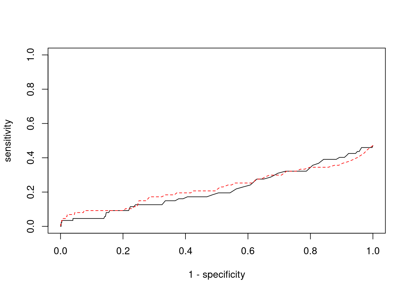
| Version | Author | Date |
|---|---|---|
| 3a7fbc1 | wesleycrouse | 2021-09-08 |
Sensitivity, specificity and precision for silver standard genes - bystanders only
This section first uses all silver standard genes to identify bystander genes within 1Mb. The silver standard and bystander gene lists are then subset to only genes with imputed expression in this analysis. Then, the ctwas and TWAS gene lists from this analysis are subset to only genes that are in the (subset) silver standard and bystander genes. These gene lists are then used to compute sensitivity, specificity and precision for ctwas and TWAS.
library(biomaRt)
library(GenomicRanges)Loading required package: stats4Loading required package: BiocGenericsLoading required package: parallel
Attaching package: 'BiocGenerics'The following objects are masked from 'package:parallel':
clusterApply, clusterApplyLB, clusterCall, clusterEvalQ,
clusterExport, clusterMap, parApply, parCapply, parLapply,
parLapplyLB, parRapply, parSapply, parSapplyLBThe following objects are masked from 'package:stats':
IQR, mad, sd, var, xtabsThe following objects are masked from 'package:base':
anyDuplicated, append, as.data.frame, basename, cbind,
colnames, dirname, do.call, duplicated, eval, evalq, Filter,
Find, get, grep, grepl, intersect, is.unsorted, lapply, Map,
mapply, match, mget, order, paste, pmax, pmax.int, pmin,
pmin.int, Position, rank, rbind, Reduce, rownames, sapply,
setdiff, sort, table, tapply, union, unique, unsplit, which,
which.max, which.minLoading required package: S4Vectors
Attaching package: 'S4Vectors'The following object is masked from 'package:base':
expand.gridLoading required package: IRangesLoading required package: GenomeInfoDbensembl <- useEnsembl(biomart="ENSEMBL_MART_ENSEMBL", dataset="hsapiens_gene_ensembl")
G_list <- getBM(filters= "chromosome_name", attributes= c("hgnc_symbol","chromosome_name","start_position","end_position","gene_biotype"), values=1:22, mart=ensembl)
G_list <- G_list[G_list$hgnc_symbol!="",]
G_list <- G_list[G_list$gene_biotype %in% c("protein_coding","lncRNA"),]
G_list$start <- G_list$start_position
G_list$end <- G_list$end_position
G_list_granges <- makeGRangesFromDataFrame(G_list, keep.extra.columns=T)
known_annotations_positions <- G_list[G_list$hgnc_symbol %in% known_annotations,]
half_window <- 1000000
known_annotations_positions$start <- known_annotations_positions$start_position - half_window
known_annotations_positions$end <- known_annotations_positions$end_position + half_window
known_annotations_positions$start[known_annotations_positions$start<1] <- 1
known_annotations_granges <- makeGRangesFromDataFrame(known_annotations_positions, keep.extra.columns=T)
bystanders <- findOverlaps(known_annotations_granges,G_list_granges)
bystanders <- unique(subjectHits(bystanders))
bystanders <- G_list$hgnc_symbol[bystanders]
bystanders <- bystanders[!(bystanders %in% known_annotations)]
unrelated_genes <- bystanders
#number of genes in known annotations
print(length(known_annotations))[1] 87#number of genes in known annotations with imputed expression
print(sum(known_annotations %in% ctwas_gene_res$genename))[1] 41#number of bystander genes
print(length(unrelated_genes))[1] 1944#number of bystander genes with imputed expression
print(sum(unrelated_genes %in% ctwas_gene_res$genename))[1] 1078#remove genes without imputed expression from gene lists
known_annotations <- known_annotations[known_annotations %in% ctwas_gene_res$genename]
unrelated_genes <- unrelated_genes[unrelated_genes %in% ctwas_gene_res$genename]
#assign ctwas and TWAS genes
ctwas_genes <- ctwas_gene_res$genename[ctwas_gene_res$susie_pip>0.8]
twas_genes <- ctwas_gene_res$genename[abs(ctwas_gene_res$z)>sig_thresh]
#significance threshold for TWAS
print(sig_thresh)[1] 4.616471#number of ctwas genes
length(ctwas_genes)[1] 14#number of ctwas genes in known annotations or bystanders
sum(ctwas_genes %in% c(known_annotations, unrelated_genes))[1] 1#number of ctwas genes
length(twas_genes)[1] 77#number of TWAS genes
sum(twas_genes %in% c(known_annotations, unrelated_genes))[1] 16#remove genes not in known or bystander lists from results
ctwas_genes <- ctwas_genes[ctwas_genes %in% c(known_annotations, unrelated_genes)]
twas_genes <- twas_genes[twas_genes %in% c(known_annotations, unrelated_genes)]
#sensitivity / recall
sensitivity <- rep(NA,2)
names(sensitivity) <- c("ctwas", "TWAS")
sensitivity["ctwas"] <- sum(ctwas_genes %in% known_annotations)/length(known_annotations)
sensitivity["TWAS"] <- sum(twas_genes %in% known_annotations)/length(known_annotations)
sensitivity
ctwas TWAS
0.00000000 0.07317073 #specificity
specificity <- rep(NA,2)
names(specificity) <- c("ctwas", "TWAS")
specificity["ctwas"] <- sum(!(unrelated_genes %in% ctwas_genes))/length(unrelated_genes)
specificity["TWAS"] <- sum(!(unrelated_genes %in% twas_genes))/length(unrelated_genes)
specificity ctwas TWAS
0.9990724 0.9879406 #precision / PPV
precision <- rep(NA,2)
names(precision) <- c("ctwas", "TWAS")
precision["ctwas"] <- sum(ctwas_genes %in% known_annotations)/length(ctwas_genes)
precision["TWAS"] <- sum(twas_genes %in% known_annotations)/length(twas_genes)
precision ctwas TWAS
0.0000 0.1875
sessionInfo()R version 3.6.1 (2019-07-05)
Platform: x86_64-pc-linux-gnu (64-bit)
Running under: Scientific Linux 7.4 (Nitrogen)
Matrix products: default
BLAS/LAPACK: /software/openblas-0.2.19-el7-x86_64/lib/libopenblas_haswellp-r0.2.19.so
locale:
[1] LC_CTYPE=en_US.UTF-8 LC_NUMERIC=C
[3] LC_TIME=en_US.UTF-8 LC_COLLATE=en_US.UTF-8
[5] LC_MONETARY=en_US.UTF-8 LC_MESSAGES=en_US.UTF-8
[7] LC_PAPER=en_US.UTF-8 LC_NAME=C
[9] LC_ADDRESS=C LC_TELEPHONE=C
[11] LC_MEASUREMENT=en_US.UTF-8 LC_IDENTIFICATION=C
attached base packages:
[1] parallel stats4 stats graphics grDevices utils datasets
[8] methods base
other attached packages:
[1] GenomicRanges_1.36.0 GenomeInfoDb_1.20.0 IRanges_2.18.1
[4] S4Vectors_0.22.1 BiocGenerics_0.30.0 biomaRt_2.40.1
[7] readxl_1.3.1 WebGestaltR_0.4.4 disgenet2r_0.99.2
[10] enrichR_3.0 cowplot_1.0.0 ggplot2_3.3.3
loaded via a namespace (and not attached):
[1] bitops_1.0-6 fs_1.3.1 bit64_4.0.5
[4] doParallel_1.0.16 progress_1.2.2 httr_1.4.1
[7] rprojroot_2.0.2 tools_3.6.1 doRNG_1.8.2
[10] utf8_1.2.1 R6_2.5.0 DBI_1.1.1
[13] colorspace_1.4-1 withr_2.4.1 tidyselect_1.1.0
[16] prettyunits_1.0.2 bit_4.0.4 curl_3.3
[19] compiler_3.6.1 git2r_0.26.1 Biobase_2.44.0
[22] labeling_0.3 scales_1.1.0 readr_1.4.0
[25] stringr_1.4.0 apcluster_1.4.8 digest_0.6.20
[28] rmarkdown_1.13 svglite_1.2.2 XVector_0.24.0
[31] pkgconfig_2.0.3 htmltools_0.3.6 fastmap_1.1.0
[34] rlang_0.4.11 RSQLite_2.2.7 farver_2.1.0
[37] generics_0.0.2 jsonlite_1.6 dplyr_1.0.7
[40] RCurl_1.98-1.1 magrittr_2.0.1 GenomeInfoDbData_1.2.1
[43] Matrix_1.2-18 Rcpp_1.0.6 munsell_0.5.0
[46] fansi_0.5.0 gdtools_0.1.9 lifecycle_1.0.0
[49] stringi_1.4.3 whisker_0.3-2 yaml_2.2.0
[52] zlibbioc_1.30.0 plyr_1.8.4 grid_3.6.1
[55] blob_1.2.1 promises_1.0.1 crayon_1.4.1
[58] lattice_0.20-38 hms_1.1.0 knitr_1.23
[61] pillar_1.6.1 igraph_1.2.4.1 rjson_0.2.20
[64] rngtools_1.5 reshape2_1.4.3 codetools_0.2-16
[67] XML_3.98-1.20 glue_1.4.2 evaluate_0.14
[70] data.table_1.14.0 vctrs_0.3.8 httpuv_1.5.1
[73] foreach_1.5.1 cellranger_1.1.0 gtable_0.3.0
[76] purrr_0.3.4 assertthat_0.2.1 cachem_1.0.5
[79] xfun_0.8 later_0.8.0 tibble_3.1.2
[82] iterators_1.0.13 AnnotationDbi_1.46.0 memoise_2.0.0
[85] workflowr_1.6.2 ellipsis_0.3.2