C-reactive protein (quantile) - Liver
wesleycrouse
2021-09-09
Last updated: 2021-09-09
Checks: 6 1
Knit directory: ctwas_applied/
This reproducible R Markdown analysis was created with workflowr (version 1.6.2). The Checks tab describes the reproducibility checks that were applied when the results were created. The Past versions tab lists the development history.
The R Markdown file has unstaged changes. To know which version of the R Markdown file created these results, you’ll want to first commit it to the Git repo. If you’re still working on the analysis, you can ignore this warning. When you’re finished, you can run wflow_publish to commit the R Markdown file and build the HTML.
Great job! The global environment was empty. Objects defined in the global environment can affect the analysis in your R Markdown file in unknown ways. For reproduciblity it’s best to always run the code in an empty environment.
The command set.seed(20210726) was run prior to running the code in the R Markdown file. Setting a seed ensures that any results that rely on randomness, e.g. subsampling or permutations, are reproducible.
Great job! Recording the operating system, R version, and package versions is critical for reproducibility.
Nice! There were no cached chunks for this analysis, so you can be confident that you successfully produced the results during this run.
Great job! Using relative paths to the files within your workflowr project makes it easier to run your code on other machines.
Great! You are using Git for version control. Tracking code development and connecting the code version to the results is critical for reproducibility.
The results in this page were generated with repository version 59e5f4d. See the Past versions tab to see a history of the changes made to the R Markdown and HTML files.
Note that you need to be careful to ensure that all relevant files for the analysis have been committed to Git prior to generating the results (you can use wflow_publish or wflow_git_commit). workflowr only checks the R Markdown file, but you know if there are other scripts or data files that it depends on. Below is the status of the Git repository when the results were generated:
Unstaged changes:
    Modified:   analysis/ukb-d-30500_irnt_Liver.Rmd
    Modified:   analysis/ukb-d-30600_irnt_Liver.Rmd
    Modified:   analysis/ukb-d-30610_irnt_Liver.Rmd
    Modified:   analysis/ukb-d-30620_irnt_Liver.Rmd
    Modified:   analysis/ukb-d-30630_irnt_Liver.Rmd
    Modified:   analysis/ukb-d-30640_irnt_Liver.Rmd
    Modified:   analysis/ukb-d-30650_irnt_Liver.Rmd
    Modified:   analysis/ukb-d-30660_irnt_Liver.Rmd
    Modified:   analysis/ukb-d-30670_irnt_Liver.Rmd
    Modified:   analysis/ukb-d-30680_irnt_Liver.Rmd
    Modified:   analysis/ukb-d-30690_irnt_Liver.Rmd
    Modified:   analysis/ukb-d-30700_irnt_Liver.Rmd
    Modified:   analysis/ukb-d-30710_irnt_Liver.Rmd
Note that any generated files, e.g. HTML, png, CSS, etc., are not included in this status report because it is ok for generated content to have uncommitted changes.
These are the previous versions of the repository in which changes were made to the R Markdown (analysis/ukb-d-30710_irnt_Liver.Rmd) and HTML (docs/ukb-d-30710_irnt_Liver.html) files. If you’ve configured a remote Git repository (see ?wflow_git_remote), click on the hyperlinks in the table below to view the files as they were in that past version.
| File | Version | Author | Date | Message |
|---|---|---|---|---|
| Rmd | cbf7408 | wesleycrouse | 2021-09-08 | adding enrichment to reports |
| html | cbf7408 | wesleycrouse | 2021-09-08 | adding enrichment to reports |
| Rmd | 4970e3e | wesleycrouse | 2021-09-08 | updating reports |
| html | 4970e3e | wesleycrouse | 2021-09-08 | updating reports |
| Rmd | 627a4e1 | wesleycrouse | 2021-09-07 | adding heritability |
| Rmd | dfd2b5f | wesleycrouse | 2021-09-07 | regenerating reports |
| html | dfd2b5f | wesleycrouse | 2021-09-07 | regenerating reports |
| Rmd | 61b53b3 | wesleycrouse | 2021-09-06 | updated PVE calculation |
| html | 61b53b3 | wesleycrouse | 2021-09-06 | updated PVE calculation |
| Rmd | 837dd01 | wesleycrouse | 2021-09-01 | adding additional fixedsigma report |
| Rmd | d0a5417 | wesleycrouse | 2021-08-30 | adding new reports to the index |
| Rmd | 0922de7 | wesleycrouse | 2021-08-18 | updating all reports with locus plots |
| html | 0922de7 | wesleycrouse | 2021-08-18 | updating all reports with locus plots |
| html | 1c62980 | wesleycrouse | 2021-08-11 | Updating reports |
| Rmd | 5981e80 | wesleycrouse | 2021-08-11 | Adding more reports |
| html | 5981e80 | wesleycrouse | 2021-08-11 | Adding more reports |
| Rmd | 05a98b7 | wesleycrouse | 2021-08-07 | adding additional results |
| html | 05a98b7 | wesleycrouse | 2021-08-07 | adding additional results |
| html | 03e541c | wesleycrouse | 2021-07-29 | Cleaning up report generation |
| Rmd | 276893d | wesleycrouse | 2021-07-29 | Updating reports |
| html | 276893d | wesleycrouse | 2021-07-29 | Updating reports |
Overview
These are the results of a ctwas analysis of the UK Biobank trait C-reactive protein (quantile) using Liver gene weights.
The GWAS was conducted by the Neale Lab, and the biomarker traits we analyzed are discussed here. Summary statistics were obtained from IEU OpenGWAS using GWAS ID: ukb-d-30710_irnt. Results were obtained from from IEU rather than Neale Lab because they are in a standardard format (GWAS VCF). Note that 3 of the 34 biomarker traits were not available from IEU and were excluded from analysis.
The weights are mashr GTEx v8 models on Liver eQTL obtained from PredictDB. We performed a full harmonization of the variants, including recovering strand ambiguous variants. This procedure is discussed in a separate document. (TO-DO: add report that describes harmonization)
LD matrices were computed from a 10% subset of Neale lab subjects. Subjects were matched using the plate and well information from genotyping. We included only biallelic variants with MAF>0.01 in the original Neale Lab GWAS. (TO-DO: add more details [number of subjects, variants, etc])
Weight QC
TO-DO: add enhanced QC reporting (total number of weights, why each variant was missing for all genes)
qclist_all <- list()

qc_files <- paste0(results_dir, "/", list.files(results_dir, pattern="exprqc.Rd"))

for (i in 1:length(qc_files)){
  load(qc_files[i])
  chr <- unlist(strsplit(rev(unlist(strsplit(qc_files[i], "_")))[1], "[.]"))[1]
  qclist_all[[chr]] <- cbind(do.call(rbind, lapply(qclist,unlist)), as.numeric(substring(chr,4)))
}

qclist_all <- data.frame(do.call(rbind, qclist_all))
colnames(qclist_all)[ncol(qclist_all)] <- "chr"

rm(qclist, wgtlist, z_gene_chr)

#number of imputed weights
nrow(qclist_all)
[1] 10901#number of imputed weights by chromosome
table(qclist_all$chr)
   1    2    3    4    5    6    7    8    9   10   11   12   13   14   15
1070  768  652  417  494  611  548  408  405  434  634  629  195  365  354
  16   17   18   19   20   21   22
 526  663  160  859  306  114  289
#proportion of imputed weights without missing variants
mean(qclist_all$nmiss==0)[1] 0.8366205Load ctwas results
#load ctwas results
ctwas_res <- data.table::fread(paste0(results_dir, "/", analysis_id, "_ctwas.susieIrss.txt"))

#make unique identifier for regions
ctwas_res$region_tag <- paste(ctwas_res$region_tag1, ctwas_res$region_tag2, sep="_")

#compute PVE for each gene/SNP
ctwas_res$PVE = ctwas_res$susie_pip*ctwas_res$mu2/sample_size #check PVE calculation

#separate gene and SNP results
ctwas_gene_res <- ctwas_res[ctwas_res$type == "gene", ]
ctwas_gene_res <- data.frame(ctwas_gene_res)
ctwas_snp_res <- ctwas_res[ctwas_res$type == "SNP", ]
ctwas_snp_res <- data.frame(ctwas_snp_res)

#add gene information to results
sqlite <- RSQLite::dbDriver("SQLite")
db = RSQLite::dbConnect(sqlite, paste0("/project2/compbio/predictdb/mashr_models/mashr_", weight, ".db"))
query <- function(...) RSQLite::dbGetQuery(db, ...)
gene_info <- query("select gene, genename from extra")
gene_info <- query("select gene, genename, gene_type from extra")
RSQLite::dbDisconnect(db)

ctwas_gene_res <- cbind(ctwas_gene_res, gene_info[sapply(ctwas_gene_res$id, match, gene_info$gene), c("genename", "gene_type")])

#add z score to results
load(paste0(results_dir, "/", analysis_id, "_expr_z_gene.Rd"))
ctwas_gene_res$z <- z_gene[ctwas_gene_res$id,]$z

#load(paste0(results_dir, "/", analysis_id, "_expr_z_snp.Rd")) #for new version, stored after harmonization
z_snp <- readRDS(paste0(results_dir, "/", trait_id, ".RDS")) #for old version, unharmonized

z_snp <- z_snp[z_snp$id %in% ctwas_snp_res$id,] #subset snps to those included in analysis, note some are duplicated, need to match which allele was used
ctwas_snp_res$z <- z_snp$z[match(ctwas_snp_res$id, z_snp$id)] #for duplicated snps, this arbitrarily uses the first allele
ctwas_snp_res$z_flag <- as.numeric(ctwas_snp_res$id %in% z_snp$id[duplicated(z_snp$id)]) #mark the unclear z scores, flag=1

#formatting and rounding for tables
ctwas_gene_res$z <- round(ctwas_gene_res$z,2)
ctwas_snp_res$z <- round(ctwas_snp_res$z,2)
ctwas_gene_res$susie_pip <- round(ctwas_gene_res$susie_pip,3)
ctwas_snp_res$susie_pip <- round(ctwas_snp_res$susie_pip,3)
ctwas_gene_res$mu2 <- round(ctwas_gene_res$mu2,2)
ctwas_snp_res$mu2 <- round(ctwas_snp_res$mu2,2)
ctwas_gene_res$PVE <- signif(ctwas_gene_res$PVE, 2)
ctwas_snp_res$PVE <- signif(ctwas_snp_res$PVE, 2)

#merge gene and snp results with added information
ctwas_gene_res$z_flag=NA
ctwas_snp_res$genename=NA
ctwas_snp_res$gene_type=NA

ctwas_res <- rbind(ctwas_gene_res,
                   ctwas_snp_res[,colnames(ctwas_gene_res)])

#store columns to report
report_cols <- colnames(ctwas_gene_res)[!(colnames(ctwas_gene_res) %in% c("type", "region_tag1", "region_tag2", "cs_index", "gene_type", "z_flag", "id", "chrom", "pos"))]
first_cols <- c("genename", "region_tag")
report_cols <- c(first_cols, report_cols[!(report_cols %in% first_cols)])

report_cols_snps <- c("id", report_cols[-1])

#get number of SNPs from s1 results; adjust for thin
ctwas_res_s1 <- data.table::fread(paste0(results_dir, "/", analysis_id, "_ctwas.s1.susieIrss.txt"))
n_snps <- sum(ctwas_res_s1$type=="SNP")/thin
rm(ctwas_res_s1)
Check convergence of parameters
library(ggplot2)
library(cowplot)
********************************************************Note: As of version 1.0.0, cowplot does not change the default ggplot2 theme anymore. To recover the previous behavior, execute:
theme_set(theme_cowplot())********************************************************load(paste0(results_dir, "/", analysis_id, "_ctwas.s2.susieIrssres.Rd"))
df <- data.frame(niter = rep(1:ncol(group_prior_rec), 2),
value = c(group_prior_rec[1,], group_prior_rec[2,]),
group = rep(c("Gene", "SNP"), each = ncol(group_prior_rec)))
df$group <- as.factor(df$group)
df$value[df$group=="SNP"] <- df$value[df$group=="SNP"]*thin #adjust parameter to account for thin argument
p_pi <- ggplot(df, aes(x=niter, y=value, group=group)) +
geom_line(aes(color=group)) +
geom_point(aes(color=group)) +
xlab("Iteration") + ylab(bquote(pi)) +
ggtitle("Prior mean") +
theme_cowplot()
df <- data.frame(niter = rep(1:ncol(group_prior_var_rec), 2),
value = c(group_prior_var_rec[1,], group_prior_var_rec[2,]),
group = rep(c("Gene", "SNP"), each = ncol(group_prior_var_rec)))
df$group <- as.factor(df$group)
p_sigma2 <- ggplot(df, aes(x=niter, y=value, group=group)) +
geom_line(aes(color=group)) +
geom_point(aes(color=group)) +
xlab("Iteration") + ylab(bquote(sigma^2)) +
ggtitle("Prior variance") +
theme_cowplot()
plot_grid(p_pi, p_sigma2)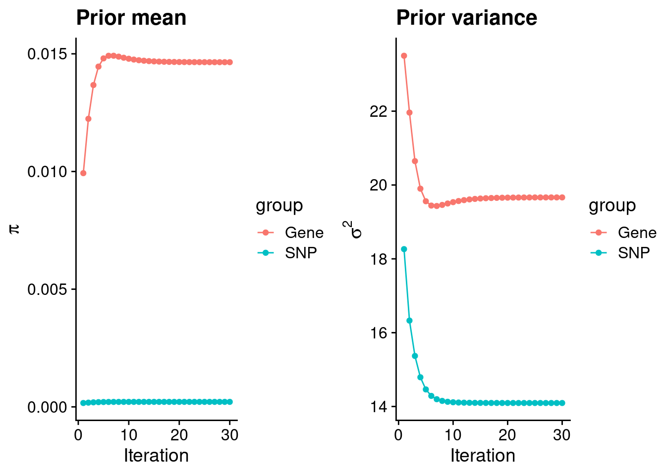
| Version | Author | Date |
|---|---|---|
| dfd2b5f | wesleycrouse | 2021-09-07 |
#estimated group prior
estimated_group_prior <- group_prior_rec[,ncol(group_prior_rec)]
names(estimated_group_prior) <- c("gene", "snp")
estimated_group_prior["snp"] <- estimated_group_prior["snp"]*thin #adjust parameter to account for thin argument
print(estimated_group_prior)
gene snp
0.0146448756 0.0002120358 #estimated group prior variance
estimated_group_prior_var <- group_prior_var_rec[,ncol(group_prior_var_rec)]
names(estimated_group_prior_var) <- c("gene", "snp")
print(estimated_group_prior_var) gene snp
19.66386 14.09507 #report sample size
print(sample_size)[1] 343524#report group size
group_size <- c(nrow(ctwas_gene_res), n_snps)
print(group_size)[1] 10901 8697330#estimated group PVE
estimated_group_pve <- estimated_group_prior_var*estimated_group_prior*group_size/sample_size #check PVE calculation
names(estimated_group_pve) <- c("gene", "snp")
print(estimated_group_pve) gene snp
0.009138266 0.075666782 #compare sum(PIP*mu2/sample_size) with above PVE calculation
c(sum(ctwas_gene_res$PVE),sum(ctwas_snp_res$PVE))[1] 0.02544839 0.62395712Genes with highest PIPs
#distribution of PIPs
hist(ctwas_gene_res$susie_pip, xlim=c(0,1), main="Distribution of Gene PIPs")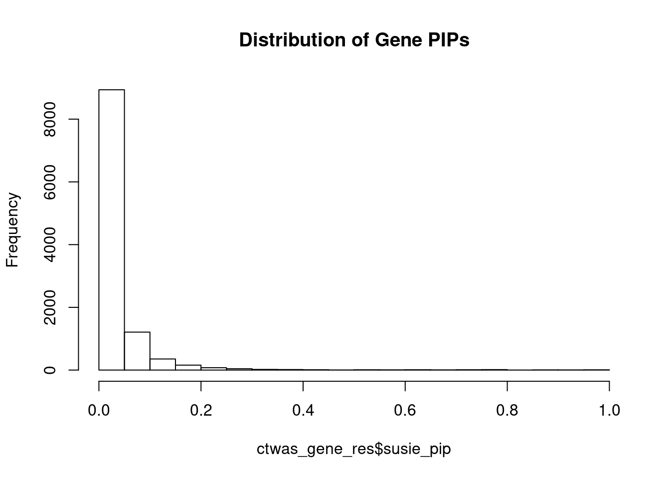
| Version | Author | Date |
|---|---|---|
| dfd2b5f | wesleycrouse | 2021-09-07 |
#genes with PIP>0.8 or 20 highest PIPs
head(ctwas_gene_res[order(-ctwas_gene_res$susie_pip),report_cols], max(sum(ctwas_gene_res$susie_pip>0.8), 20))
genename region_tag susie_pip mu2 PVE z
1231 PABPC4 1_24 0.993 106.82 3.1e-04 -10.77
10912 STARD10 11_41 0.992 58.98 1.7e-04 7.68
12467 RP11-219B17.3 15_27 0.989 147.89 4.3e-04 -12.39
4588 PPP1R1A 12_34 0.985 28.54 8.2e-05 -4.98
12102 RP11-806H10.4 17_44 0.985 76.61 2.2e-04 11.20
8489 RNASEH2C 11_36 0.971 31.75 9.0e-05 -5.45
3212 CCND2 12_4 0.971 23.43 6.6e-05 -4.51
2891 SNX17 2_16 0.969 146.27 4.1e-04 -15.95
4223 DNAJB1 19_12 0.950 31.25 8.6e-05 -5.12
886 IL4R 16_22 0.933 55.57 1.5e-04 -7.51
5143 SBNO1 12_75 0.920 42.47 1.1e-04 5.82
5127 SMARCC2 12_35 0.907 23.93 6.3e-05 4.86
11790 CYP2A6 19_28 0.901 22.94 6.0e-05 5.05
9496 KCNJ12 17_16 0.896 21.14 5.5e-05 -4.25
3620 CHST8 19_23 0.885 23.15 6.0e-05 4.44
7905 VASN 16_4 0.882 21.71 5.6e-05 -4.36
7798 ZNF526 19_29 0.865 22.34 5.6e-05 4.50
8040 THBS3 1_76 0.862 33.95 8.5e-05 5.78
9889 ZNF793 19_26 0.851 34.11 8.5e-05 -5.79
3305 C10orf76 10_65 0.814 23.55 5.6e-05 4.70Genes with largest effect sizes
#plot PIP vs effect size
plot(ctwas_gene_res$susie_pip, ctwas_gene_res$mu2, xlab="PIP", ylab="mu^2", main="Gene PIPs vs Effect Size")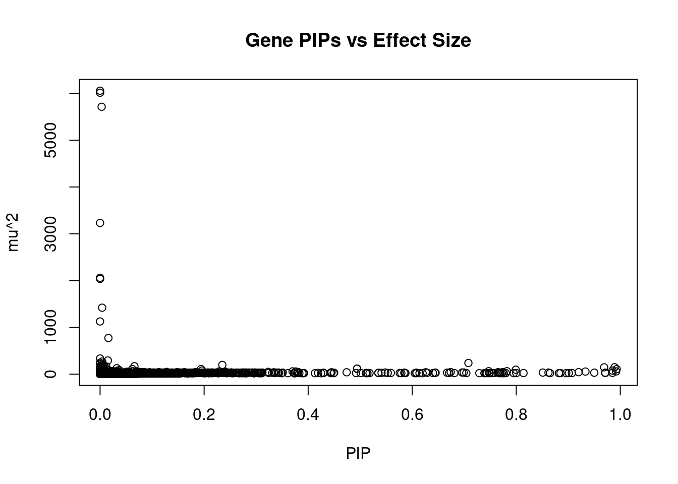
| Version | Author | Date |
|---|---|---|
| dfd2b5f | wesleycrouse | 2021-09-07 |
#genes with 20 largest effect sizes
head(ctwas_gene_res[order(-ctwas_gene_res$mu2),report_cols],20)
genename region_tag susie_pip mu2 PVE z
10186 ZGPAT 20_38 0.000 6057.22 4.6e-10 5.46
3715 SLC2A4RG 20_38 0.000 6013.93 1.6e-12 5.46
1647 ARFRP1 20_38 0.003 5713.63 4.8e-05 7.49
11199 LINC00271 6_89 0.000 3231.54 0.0e+00 -2.43
11853 RTEL1 20_38 0.000 2059.01 0.0e+00 5.66
1641 GMEB2 20_38 0.000 2035.54 0.0e+00 -4.34
4547 HNF1A 12_74 0.004 1420.42 1.8e-05 53.53
4604 AHI1 6_89 0.000 1126.25 0.0e+00 -1.88
4556 TMEM60 7_49 0.016 772.26 3.6e-05 -2.13
4299 APCS 1_78 0.000 335.17 1.8e-09 1.90
10840 PPP1CB 2_17 0.015 292.69 1.3e-05 2.89
2887 NRBP1 2_16 0.004 269.15 2.9e-06 19.36
10242 STMN3 20_38 0.000 242.65 0.0e+00 1.44
8270 TRMT61B 2_17 0.708 238.88 4.9e-04 -4.08
10551 LIME1 20_38 0.000 217.80 0.0e+00 -7.73
7172 SPDYA 2_17 0.006 204.87 3.4e-06 -3.06
8531 TNKS 8_12 0.235 197.16 1.3e-04 19.20
6936 RAVER2 1_41 0.002 191.46 1.0e-06 -7.30
8284 RBKS 2_16 0.066 168.95 3.2e-05 15.74
11738 RP11-115J16.2 8_12 0.004 164.78 2.1e-06 13.24Genes with highest PVE
#genes with 20 highest pve
head(ctwas_gene_res[order(-ctwas_gene_res$PVE),report_cols],20)
genename region_tag susie_pip mu2 PVE z
8270 TRMT61B 2_17 0.708 238.88 4.9e-04 -4.08
12467 RP11-219B17.3 15_27 0.989 147.89 4.3e-04 -12.39
2891 SNX17 2_16 0.969 146.27 4.1e-04 -15.95
1231 PABPC4 1_24 0.993 106.82 3.1e-04 -10.77
6792 ADAR 1_75 0.799 94.90 2.2e-04 13.57
12102 RP11-806H10.4 17_44 0.985 76.61 2.2e-04 11.20
1058 GCKR 2_16 0.494 116.71 1.7e-04 -14.72
10987 C2orf16 2_16 0.494 116.71 1.7e-04 -14.72
10912 STARD10 11_41 0.992 58.98 1.7e-04 7.68
886 IL4R 16_22 0.933 55.57 1.5e-04 -7.51
290 NR1H3 11_29 0.747 63.09 1.4e-04 -9.89
666 COASY 17_25 0.782 62.34 1.4e-04 6.76
8531 TNKS 8_12 0.235 197.16 1.3e-04 19.20
5143 SBNO1 12_75 0.920 42.47 1.1e-04 5.82
4925 IFT172 2_16 0.774 44.86 1.0e-04 7.85
8685 KCTD13 16_24 0.765 42.66 9.5e-05 6.39
8489 RNASEH2C 11_36 0.971 31.75 9.0e-05 -5.45
7241 MST1R 3_35 0.674 44.61 8.8e-05 8.81
4223 DNAJB1 19_12 0.950 31.25 8.6e-05 -5.12
8040 THBS3 1_76 0.862 33.95 8.5e-05 5.78Genes with largest z scores
#genes with 20 largest z scores
head(ctwas_gene_res[order(-abs(ctwas_gene_res$z)),report_cols],20)
genename region_tag susie_pip mu2 PVE z
4547 HNF1A 12_74 0.004 1420.42 1.8e-05 53.53
9534 PDE4B 1_41 0.000 141.57 3.0e-15 -20.55
2887 NRBP1 2_16 0.004 269.15 2.9e-06 19.36
8531 TNKS 8_12 0.235 197.16 1.3e-04 19.20
2891 SNX17 2_16 0.969 146.27 4.1e-04 -15.95
8284 RBKS 2_16 0.066 168.95 3.2e-05 15.74
1058 GCKR 2_16 0.494 116.71 1.7e-04 -14.72
10987 C2orf16 2_16 0.494 116.71 1.7e-04 -14.72
4550 P2RX4 12_74 0.004 87.70 1.1e-06 -14.28
6792 ADAR 1_75 0.799 94.90 2.2e-04 13.57
11738 RP11-115J16.2 8_12 0.004 164.78 2.1e-06 13.24
12467 RP11-219B17.3 15_27 0.989 147.89 4.3e-04 -12.39
1455 JOSD1 22_15 0.032 126.81 1.2e-05 -12.08
1447 DDX17 22_15 0.007 104.82 2.0e-06 -11.66
4936 SLC5A6 2_16 0.011 124.70 4.0e-06 11.42
7115 AIM2 1_78 0.000 135.73 0.0e+00 11.30
4941 ATRAID 2_16 0.008 118.09 2.8e-06 -11.25
12102 RP11-806H10.4 17_44 0.985 76.61 2.2e-04 11.20
5511 ATP8B2 1_75 0.062 108.67 2.0e-05 -10.98
10597 HLA-DRA 6_26 0.002 31.11 1.6e-07 -10.85Comparing z scores and PIPs
#set nominal signifiance threshold for z scores
alpha <- 0.05

#bonferroni adjusted threshold for z scores
sig_thresh <- qnorm(1-(alpha/nrow(ctwas_gene_res)/2), lower=T)

#Q-Q plot for z scores
obs_z <- ctwas_gene_res$z[order(ctwas_gene_res$z)]
exp_z <- qnorm((1:nrow(ctwas_gene_res))/nrow(ctwas_gene_res))

plot(exp_z, obs_z, xlab="Expected z", ylab="Observed z", main="Gene z score Q-Q plot")
abline(a=0,b=1)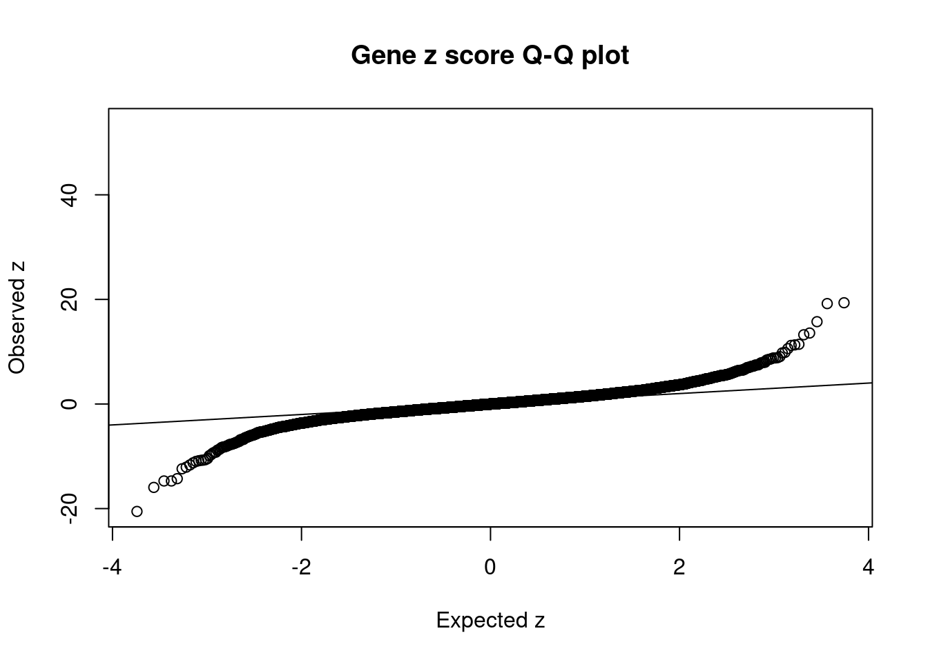
| Version | Author | Date |
|---|---|---|
| dfd2b5f | wesleycrouse | 2021-09-07 |
#plot z score vs PIP
plot(abs(ctwas_gene_res$z), ctwas_gene_res$susie_pip, xlab="abs(z)", ylab="PIP")
abline(v=sig_thresh, col="red", lty=2)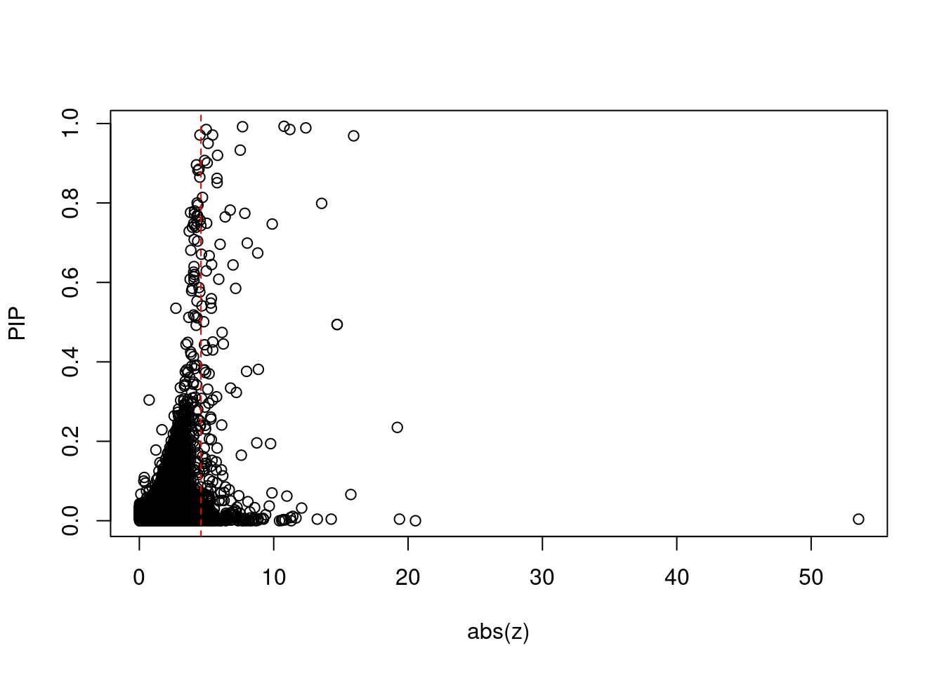
| Version | Author | Date |
|---|---|---|
| dfd2b5f | wesleycrouse | 2021-09-07 |
#proportion of significant z scores
mean(abs(ctwas_gene_res$z) > sig_thresh)
[1] 0.02412623#genes with most significant z scores
head(ctwas_gene_res[order(-abs(ctwas_gene_res$z)),report_cols],20) genename region_tag susie_pip mu2 PVE z
4547 HNF1A 12_74 0.004 1420.42 1.8e-05 53.53
9534 PDE4B 1_41 0.000 141.57 3.0e-15 -20.55
2887 NRBP1 2_16 0.004 269.15 2.9e-06 19.36
8531 TNKS 8_12 0.235 197.16 1.3e-04 19.20
2891 SNX17 2_16 0.969 146.27 4.1e-04 -15.95
8284 RBKS 2_16 0.066 168.95 3.2e-05 15.74
1058 GCKR 2_16 0.494 116.71 1.7e-04 -14.72
10987 C2orf16 2_16 0.494 116.71 1.7e-04 -14.72
4550 P2RX4 12_74 0.004 87.70 1.1e-06 -14.28
6792 ADAR 1_75 0.799 94.90 2.2e-04 13.57
11738 RP11-115J16.2 8_12 0.004 164.78 2.1e-06 13.24
12467 RP11-219B17.3 15_27 0.989 147.89 4.3e-04 -12.39
1455 JOSD1 22_15 0.032 126.81 1.2e-05 -12.08
1447 DDX17 22_15 0.007 104.82 2.0e-06 -11.66
4936 SLC5A6 2_16 0.011 124.70 4.0e-06 11.42
7115 AIM2 1_78 0.000 135.73 0.0e+00 11.30
4941 ATRAID 2_16 0.008 118.09 2.8e-06 -11.25
12102 RP11-806H10.4 17_44 0.985 76.61 2.2e-04 11.20
5511 ATP8B2 1_75 0.062 108.67 2.0e-05 -10.98
10597 HLA-DRA 6_26 0.002 31.11 1.6e-07 -10.85Locus plots for genes and SNPs
ctwas_gene_res_sortz <- ctwas_gene_res[order(-abs(ctwas_gene_res$z)),]

n_plots <- 5
for (region_tag_plot in head(unique(ctwas_gene_res_sortz$region_tag), n_plots)){
  ctwas_res_region <-  ctwas_res[ctwas_res$region_tag==region_tag_plot,]
  start <- min(ctwas_res_region$pos)
  end <- max(ctwas_res_region$pos)

  ctwas_res_region <- ctwas_res_region[order(ctwas_res_region$pos),]
  ctwas_res_region_gene <- ctwas_res_region[ctwas_res_region$type=="gene",]
  ctwas_res_region_snp <- ctwas_res_region[ctwas_res_region$type=="SNP",]

  #region name
  print(paste0("Region: ", region_tag_plot))

  #table of genes in region
  print(ctwas_res_region_gene[,report_cols])

  par(mfrow=c(4,1))

  #gene z scores
  plot(ctwas_res_region_gene$pos, abs(ctwas_res_region_gene$z), xlab="Position", ylab="abs(gene_z)", xlim=c(start,end),
   ylim=c(0,max(sig_thresh, abs(ctwas_res_region_gene$z))),
   main=paste0("Region: ", region_tag_plot))
  abline(h=sig_thresh,col="red",lty=2)

  #significance threshold for SNPs
  alpha_snp <- 5*10^(-8)
  sig_thresh_snp <- qnorm(1-alpha_snp/2, lower=T)

  #snp z scores
  plot(ctwas_res_region_snp$pos, abs(ctwas_res_region_snp$z), xlab="Position", ylab="abs(snp_z)",xlim=c(start,end),
   ylim=c(0,max(sig_thresh_snp, max(abs(ctwas_res_region_snp$z)))))
  abline(h=sig_thresh_snp,col="purple",lty=2)

  #gene pips
  plot(ctwas_res_region_gene$pos, ctwas_res_region_gene$susie_pip, xlab="Position", ylab="Gene PIP", xlim=c(start,end), ylim=c(0,1))
  abline(h=0.8,col="blue",lty=2)

  #snp pips
  plot(ctwas_res_region_snp$pos, ctwas_res_region_snp$susie_pip, xlab="Position", ylab="SNP PIP", xlim=c(start,end), ylim=c(0,1))
  abline(h=0.8,col="blue",lty=2)
}
[1] "Region: 12_74"
genename region_tag susie_pip mu2 PVE z
11059 TMEM233 12_74 0.032 47.24 4.4e-06 5.08
11597 RP11-768F21.1 12_74 0.068 48.27 9.5e-06 4.14
2588 PRKAB1 12_74 0.001 13.78 4.1e-08 1.92
3514 CIT 12_74 0.001 6.27 9.9e-09 -1.60
2591 RAB35 12_74 0.002 22.49 9.9e-08 3.70
1184 GCN1 12_74 0.001 7.00 1.1e-08 0.49
1185 RPLP0 12_74 0.001 8.25 1.6e-08 -3.46
1186 PXN 12_74 0.001 46.15 1.0e-07 8.81
1187 SIRT4 12_74 0.005 65.01 9.2e-07 -8.84
4546 MSI1 12_74 0.001 7.60 1.2e-08 2.94
2593 COX6A1 12_74 0.001 17.61 2.9e-08 2.24
8244 TRIAP1 12_74 0.001 11.57 2.6e-08 2.07
11829 GATC 12_74 0.001 6.57 1.2e-08 -2.38
1170 DYNLL1 12_74 0.001 15.26 4.7e-08 0.97
2504 COQ5 12_74 0.001 15.60 4.0e-08 3.36
7747 POP5 12_74 0.001 14.62 2.6e-08 -4.14
2510 MLEC 12_74 0.001 49.75 7.7e-08 2.90
12607 RP11-173P15.9 12_74 0.001 35.29 8.3e-08 1.15
12570 RP11-173P15.10 12_74 0.001 109.93 1.8e-07 -10.64
3516 ACADS 12_74 0.001 49.79 1.0e-07 10.59
4547 HNF1A 12_74 0.004 1420.42 1.8e-05 53.53
4549 OASL 12_74 0.001 27.55 4.7e-08 -4.48
1176 P2RX7 12_74 0.034 48.16 4.8e-06 -4.48
12471 RP11-340F14.6 12_74 0.001 23.78 4.4e-08 6.15
4550 P2RX4 12_74 0.004 87.70 1.1e-06 -14.28
2512 CAMKK2 12_74 0.004 69.52 8.3e-07 -9.24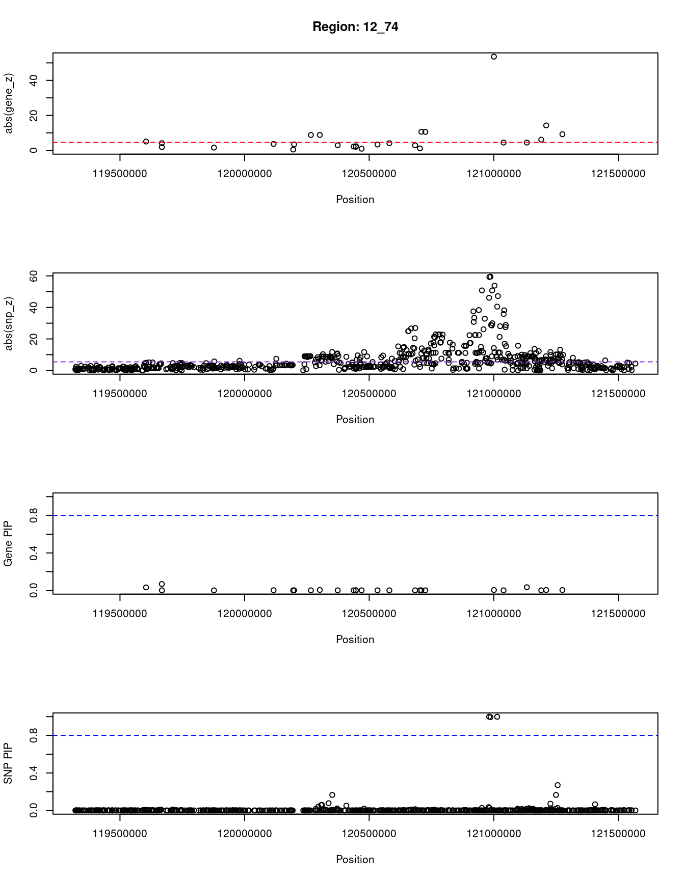
| Version | Author | Date |
|---|---|---|
| dfd2b5f | wesleycrouse | 2021-09-07 |
[1] "Region: 1_41"
     genename region_tag susie_pip    mu2     PVE      z
6936   RAVER2       1_41     0.002 191.46 1.0e-06  -7.30
6935     JAK1       1_41     0.000   7.41 1.5e-16   0.94
6934      AK4       1_41     0.000   7.98 1.9e-16  -0.34
9534    PDE4B       1_41     0.000 141.57 3.0e-15 -20.55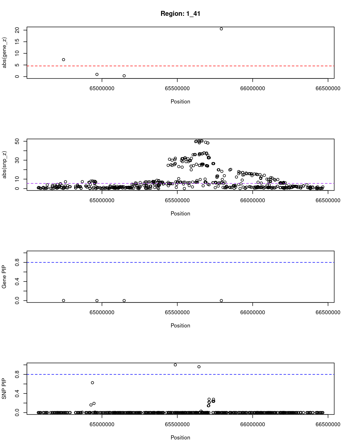
| Version | Author | Date |
|---|---|---|
| dfd2b5f | wesleycrouse | 2021-09-07 |
[1] "Region: 2_16"
      genename region_tag susie_pip    mu2     PVE      z
2881     CENPA       2_16     0.010  22.86 6.6e-07   3.73
11149     OST4       2_16     0.005  15.92 2.3e-07   2.27
4939   EMILIN1       2_16     0.002  27.58 1.7e-07  -6.25
4927       KHK       2_16     0.004  15.29 2.0e-07   2.52
4935      PREB       2_16     0.011  53.71 1.7e-06   7.16
4941    ATRAID       2_16     0.008 118.09 2.8e-06 -11.25
4936    SLC5A6       2_16     0.011 124.70 4.0e-06  11.42
1060       CAD       2_16     0.004  72.42 7.7e-07   7.45
2885   SLC30A3       2_16     0.002  50.50 2.6e-07   8.39
7169       UCN       2_16     0.012  30.53 1.1e-06   6.54
2891     SNX17       2_16     0.969 146.27 4.1e-04 -15.95
7170    ZNF513       2_16     0.008  66.39 1.6e-06   5.57
2887     NRBP1       2_16     0.004 269.15 2.9e-06  19.36
4925    IFT172       2_16     0.774  44.86 1.0e-04   7.85
1058      GCKR       2_16     0.494 116.71 1.7e-04 -14.72
10987  C2orf16       2_16     0.494 116.71 1.7e-04 -14.72
10407     GPN1       2_16     0.005  84.54 1.2e-06   9.06
8847   CCDC121       2_16     0.005  29.18 4.0e-07  -4.39
6575       BRE       2_16     0.027  38.79 3.1e-06  -7.13
8284      RBKS       2_16     0.066 168.95 3.2e-05  15.74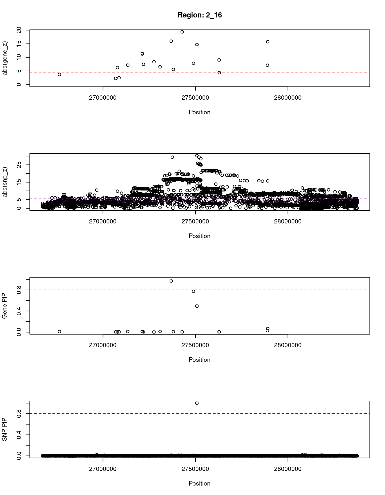
| Version | Author | Date |
|---|---|---|
| dfd2b5f | wesleycrouse | 2021-09-07 |
[1] "Region: 8_12"
           genename region_tag susie_pip    mu2     PVE     z
8531           TNKS       8_12     0.235 197.16 1.3e-04 19.20
11738 RP11-115J16.2       8_12     0.004 164.78 2.1e-06 13.24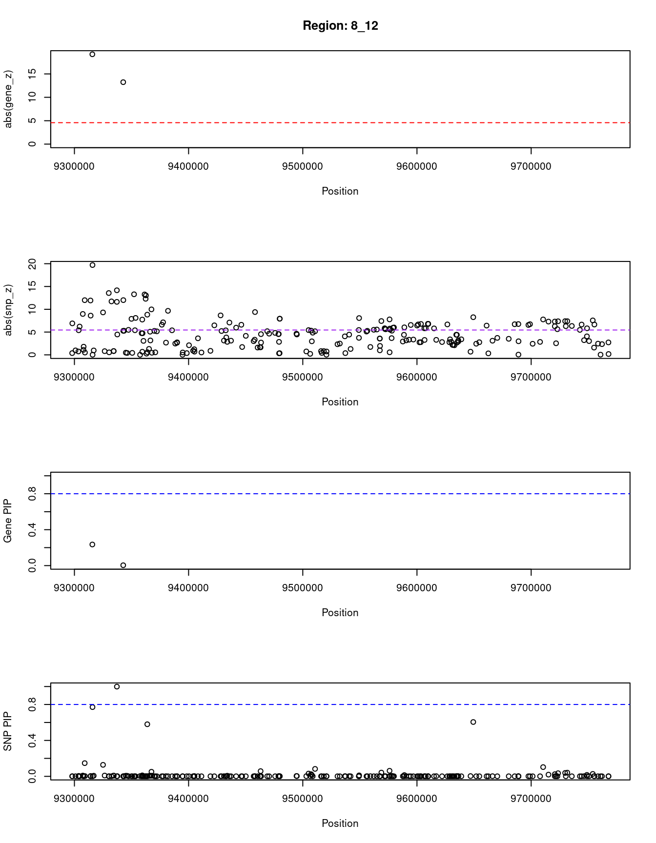
| Version | Author | Date |
|---|---|---|
| dfd2b5f | wesleycrouse | 2021-09-07 |
[1] "Region: 1_75"
      genename region_tag susie_pip    mu2     PVE      z
10541      LOR       1_75     0.000  12.26 1.3e-08   1.15
7058    S100A9       1_75     0.000   5.02 2.7e-09   0.75
5516    S100A8       1_75     0.000   4.86 2.7e-09   0.58
9867    S100A3       1_75     0.000   5.17 2.9e-09  -0.21
10028   S100A4       1_75     0.000   5.23 3.0e-09  -0.16
10140   S100A2       1_75     0.000   7.75 5.5e-09   0.84
9936   S100A16       1_75     0.001  25.41 6.1e-08  -4.35
10003  S100A14       1_75     0.001  21.58 3.1e-08   4.35
6786    S100A1       1_75     0.001  21.83 3.6e-08   4.28
9994   S100A13       1_75     0.000  18.41 1.9e-08  -3.80
6787     CHTOP       1_75     0.000  15.34 1.4e-08  -3.61
5517    SNAPIN       1_75     0.000  11.45 1.1e-08   2.90
8060      NPR1       1_75     0.000  17.90 2.1e-08   4.22
5528     INTS3       1_75     0.000  11.70 1.2e-08  -0.64
5526   GATAD2B       1_75     0.000   6.55 3.6e-09  -2.14
10477  DENND4B       1_75     0.005  71.68 1.1e-06  -7.56
5520   SLC39A1       1_75     0.000  13.62 1.2e-08  -3.77
5522   CREB3L4       1_75     0.000  13.62 1.2e-08  -3.77
5515     RAB13       1_75     0.000   5.84 3.2e-09  -1.77
5519    UBAP2L       1_75     0.000  34.43 4.1e-08  -4.27
5521      HAX1       1_75     0.000  11.50 1.3e-08  -1.57
5511    ATP8B2       1_75     0.062 108.67 2.0e-05 -10.98
7061    TDRD10       1_75     0.000  63.36 5.9e-08  -7.69
8049       SHE       1_75     0.000  25.73 1.4e-08   5.94
6792      ADAR       1_75     0.799  94.90 2.2e-04  13.57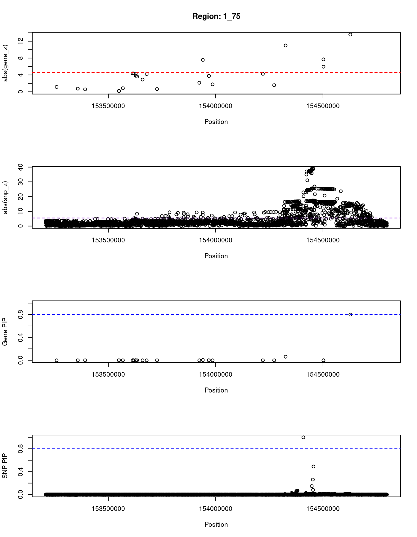
| Version | Author | Date |
|---|---|---|
| dfd2b5f | wesleycrouse | 2021-09-07 |
SNPs with highest PIPs
#snps with PIP>0.8 or 20 highest PIPs
head(ctwas_snp_res[order(-ctwas_snp_res$susie_pip),report_cols_snps],
max(sum(ctwas_snp_res$susie_pip>0.8), 20))
id region_tag susie_pip mu2 PVE z
6872 rs1772722 1_15 1.000 38.56 1.1e-04 -5.08
8327 rs79598313 1_18 1.000 111.24 3.2e-04 -11.02
17358 rs11811946 1_41 1.000 574.51 1.7e-03 32.07
36004 rs12036827 1_78 1.000 320.85 9.3e-04 6.61
36042 rs7551731 1_78 1.000 3262.96 9.5e-03 -68.36
51446 rs78270913 1_106 1.000 822.28 2.4e-03 -2.05
51464 rs61820396 1_106 1.000 783.63 2.3e-03 -2.65
59912 rs4006577 1_122 1.000 34.71 1.0e-04 -5.80
64178 rs12048215 1_131 1.000 80.25 2.3e-04 9.45
64190 rs12239046 1_131 1.000 195.36 5.7e-04 16.09
64191 rs114193355 1_131 1.000 51.25 1.5e-04 -9.08
73863 rs569546056 2_17 1.000 379.07 1.1e-03 -2.15
89068 rs6737957 2_47 1.000 559.91 1.6e-03 -4.51
89076 rs550064763 2_47 1.000 810.30 2.4e-03 -1.38
115033 rs1862069 2_102 1.000 70.34 2.0e-04 8.97
133474 rs142215640 2_136 1.000 220.21 6.4e-04 3.76
309564 rs4958888 5_88 1.000 40.64 1.2e-04 5.56
316665 rs10866657 5_103 1.000 39.23 1.1e-04 -6.89
366007 rs199804242 6_89 1.000 14134.74 4.1e-02 4.09
366502 rs62432712 6_91 1.000 49.02 1.4e-04 7.23
387798 rs11983782 7_20 1.000 78.58 2.3e-04 -8.97
403738 rs761767938 7_49 1.000 870.09 2.5e-03 1.70
403746 rs1544459 7_49 1.000 850.58 2.5e-03 2.10
433323 rs1703982 8_11 1.000 316.69 9.2e-04 -7.50
433349 rs758184196 8_11 1.000 354.98 1.0e-03 -2.22
562524 rs34623292 11_10 1.000 67.44 2.0e-04 8.73
627514 rs55692966 12_56 1.000 94.31 2.7e-04 -10.80
635435 rs1169286 12_74 1.000 893.52 2.6e-03 -46.10
695499 rs73349296 14_50 1.000 45.95 1.3e-04 -7.23
707688 rs72743115 15_22 1.000 54.98 1.6e-04 -7.51
733068 rs11641493 16_27 1.000 85.04 2.5e-04 -6.81
733069 rs112848702 16_27 1.000 100.53 2.9e-04 -8.99
733093 rs62039688 16_27 1.000 259.87 7.6e-04 -15.21
733175 rs17616063 16_27 1.000 766.81 2.2e-03 -27.92
756483 rs3110630 17_22 1.000 47.83 1.4e-04 -2.60
756484 rs12938438 17_22 1.000 86.59 2.5e-04 -4.93
756485 rs2189303 17_22 1.000 58.62 1.7e-04 2.36
763767 rs1801689 17_38 1.000 68.77 2.0e-04 8.52
784986 rs1217565 18_30 1.000 56.16 1.6e-04 -8.10
805272 rs116881820 19_32 1.000 547.46 1.6e-03 -30.35
805277 rs405509 19_32 1.000 2189.10 6.4e-03 19.05
805278 rs440446 19_32 1.000 2291.43 6.7e-03 -28.59
805281 rs814573 19_32 1.000 2308.17 6.7e-03 -73.69
838070 rs2836882 21_18 1.000 124.36 3.6e-04 -11.70
868071 rs12083537 1_75 1.000 294.86 8.6e-04 -22.86
873461 rs1260326 2_16 1.000 552.68 1.6e-03 -30.27
976807 rs11658269 17_44 1.000 136.06 4.0e-04 10.47
1010181 rs202143810 20_38 1.000 6133.64 1.8e-02 -5.38
1029067 rs6519133 22_15 1.000 142.58 4.1e-04 -13.58
31646 rs2618039 1_69 0.999 35.52 1.0e-04 5.92
329091 rs9379832 6_20 0.999 56.08 1.6e-04 -8.29
336530 rs9471632 6_32 0.999 35.20 1.0e-04 5.93
433614 rs13265179 8_12 0.999 181.87 5.3e-04 -14.17
602705 rs12824533 12_11 0.999 31.52 9.2e-05 -5.50
635450 rs2258043 12_74 0.999 688.68 2.0e-03 -40.50
687672 rs2074648 14_34 0.999 43.81 1.3e-04 6.02
707682 rs8040040 15_22 0.999 61.98 1.8e-04 -6.81
333975 rs41258084 6_27 0.998 35.25 1.0e-04 6.46
713513 rs62009152 15_36 0.998 30.76 8.9e-05 -5.07
719562 rs6496132 15_46 0.998 30.00 8.7e-05 5.27
17716 rs4655616 1_42 0.997 45.54 1.3e-04 6.30
36040 rs77289344 1_78 0.997 710.68 2.1e-03 42.02
52894 rs1223802 1_108 0.997 34.88 1.0e-04 -6.06
433889 rs506276 8_13 0.996 56.33 1.6e-04 9.82
635438 rs2393775 12_74 0.995 1841.42 5.3e-03 59.51
806527 rs601338 19_33 0.995 97.47 2.8e-04 10.26
51488 rs113267426 1_106 0.994 48.47 1.4e-04 -0.88
748864 rs71368518 17_5 0.994 28.95 8.4e-05 -4.87
64186 rs77795397 1_131 0.993 60.12 1.7e-04 0.98
137120 rs12619647 2_144 0.992 37.01 1.1e-04 6.21
418335 rs3757387 7_78 0.992 33.12 9.6e-05 5.71
687714 rs61986270 14_34 0.992 32.33 9.3e-05 4.81
7630 rs10794644 1_17 0.991 36.00 1.0e-04 -6.01
6886 rs72660319 1_15 0.987 39.09 1.1e-04 5.22
387904 rs11770879 7_20 0.987 37.18 1.1e-04 -6.65
55126 rs7523735 1_112 0.986 58.06 1.7e-04 -7.82
322359 rs10458103 6_7 0.985 39.18 1.1e-04 6.37
803897 rs1688031 19_24 0.985 46.93 1.3e-04 -6.75
93238 rs4441469 2_54 0.984 27.69 7.9e-05 5.15
921137 rs34181556 12_75 0.984 39.00 1.1e-04 4.40
84994 rs4672266 2_39 0.983 26.97 7.7e-05 -4.67
511765 rs115478735 9_70 0.983 111.89 3.2e-04 10.52
629876 rs4764939 12_62 0.981 53.73 1.5e-04 -7.45
829317 rs8121794 20_37 0.979 31.05 8.9e-05 5.53
291532 rs56821385 5_55 0.978 26.13 7.4e-05 4.92
469454 rs6987702 8_83 0.978 103.94 3.0e-04 6.94
178185 rs28433979 3_81 0.974 26.72 7.6e-05 5.09
539234 rs1269867 10_50 0.974 28.65 8.1e-05 -5.25
976832 rs41522945 17_44 0.973 51.02 1.4e-04 -7.20
606745 rs11047225 12_17 0.970 40.68 1.1e-04 6.41
561954 rs10831676 11_9 0.969 38.17 1.1e-04 -6.14
198647 rs113314116 3_121 0.968 34.08 9.6e-05 2.11
302211 rs6595550 5_76 0.968 27.08 7.6e-05 -5.06
666279 rs76620584 13_52 0.968 26.13 7.4e-05 -4.94
98770 rs72831808 2_67 0.966 30.88 8.7e-05 -5.09
829579 rs62206958 20_37 0.962 25.59 7.2e-05 4.91
17413 rs200241668 1_41 0.960 1432.90 4.0e-03 -50.44
689011 rs2270420 14_36 0.957 24.12 6.7e-05 4.49
329077 rs115740542 6_20 0.956 31.52 8.8e-05 6.76
784513 rs377181240 18_30 0.956 28.15 7.8e-05 5.17
824890 rs6020459 20_30 0.955 47.27 1.3e-04 6.99
511160 rs2966361 9_69 0.953 26.08 7.2e-05 4.96
824106 rs6066487 20_29 0.952 26.06 7.2e-05 -4.30
609649 rs60798338 12_21 0.951 58.40 1.6e-04 -5.84
366006 rs2327654 6_89 0.949 14086.90 3.9e-02 4.19
380822 rs13227497 7_9 0.947 28.22 7.8e-05 5.08
55410 rs12726661 1_113 0.944 35.70 9.8e-05 -6.07
10729 rs3103771 1_25 0.940 27.35 7.5e-05 -4.84
794667 rs111334206 19_4 0.940 25.17 6.9e-05 -4.71
328895 rs75080831 6_19 0.939 31.72 8.7e-05 5.55
98826 rs17628215 2_67 0.937 29.57 8.1e-05 5.03
333780 rs6916779 6_27 0.936 74.43 2.0e-04 6.96
387691 rs6973240 7_20 0.936 37.44 1.0e-04 4.60
503011 rs2777804 9_52 0.932 32.64 8.9e-05 5.56
747660 rs35316912 17_2 0.932 33.48 9.1e-05 5.84
355304 rs9496567 6_67 0.930 24.94 6.8e-05 4.73
469456 rs4604455 8_83 0.930 25.10 6.8e-05 -2.33
829669 rs6122476 20_37 0.926 24.03 6.5e-05 4.83
229374 rs149027545 4_59 0.924 31.86 8.6e-05 -5.59
6834 rs192212396 1_15 0.923 25.27 6.8e-05 -4.52
724848 rs6501005 16_8 0.922 24.35 6.5e-05 4.63
462694 rs35521407 8_69 0.921 42.32 1.1e-04 6.61
168787 rs138332280 3_64 0.919 26.28 7.0e-05 5.31
793626 rs351988 19_2 0.919 27.86 7.5e-05 -5.07
410125 rs10257273 7_61 0.916 90.76 2.4e-04 -8.05
215777 rs12498157 4_35 0.915 25.19 6.7e-05 4.52
475117 rs1078141 8_92 0.913 30.68 8.2e-05 5.41
837522 rs7278676 21_18 0.913 28.98 7.7e-05 5.14
606744 rs11047224 12_17 0.911 54.79 1.5e-04 -8.45
127707 rs1441171 2_126 0.908 83.15 2.2e-04 -9.41
996491 rs11666245 19_26 0.902 46.09 1.2e-04 -6.80
73759 rs7606480 2_17 0.900 29.81 7.8e-05 -5.66
572286 rs35243581 11_27 0.899 42.65 1.1e-04 6.51
141477 rs2279440 3_7 0.897 39.52 1.0e-04 6.48
221479 rs116774130 4_45 0.896 24.34 6.3e-05 -4.41
17700 rs2166311 1_42 0.891 25.31 6.6e-05 -3.44
200388 rs3752442 4_4 0.884 28.84 7.4e-05 5.35
847828 rs112169312 22_17 0.882 40.34 1.0e-04 -7.05
466521 rs2737251 8_78 0.881 68.29 1.8e-04 -9.54
98758 rs45487895 2_67 0.876 25.52 6.5e-05 -3.12
797533 rs113439314 19_9 0.873 37.24 9.5e-05 5.91
290517 rs7444298 5_52 0.868 28.69 7.2e-05 -5.06
203479 rs150164330 4_11 0.866 23.89 6.0e-05 -4.55
613733 rs2429465 12_29 0.861 25.54 6.4e-05 -4.57
113517 rs9287838 2_99 0.857 24.87 6.2e-05 -4.60
285164 rs200933157 5_42 0.857 28.53 7.1e-05 4.96
146556 rs2362186 3_18 0.854 25.70 6.4e-05 -4.58
805265 rs2972559 19_32 0.851 221.21 5.5e-04 -24.15
95673 rs12712127 2_60 0.848 43.07 1.1e-04 -6.99
337063 rs3024991 6_33 0.843 25.69 6.3e-05 4.83
208820 rs34811474 4_21 0.840 24.89 6.1e-05 -4.61
804119 rs7254601 19_24 0.840 27.11 6.6e-05 -4.80
64163 rs10737802 1_131 0.838 42.17 1.0e-04 -5.71
592687 rs68170644 11_69 0.838 27.78 6.8e-05 -4.69
635783 rs4765621 12_76 0.835 26.20 6.4e-05 -4.88
632430 rs75622376 12_67 0.832 23.88 5.8e-05 -4.36
723700 rs1436387 16_6 0.829 26.22 6.3e-05 4.80
746298 rs904787 16_53 0.824 55.80 1.3e-04 7.51
387748 rs7782803 7_20 0.821 77.11 1.8e-04 -8.01
626760 rs35000205 12_55 0.821 27.43 6.6e-05 4.92
146936 rs11711833 3_18 0.820 27.79 6.6e-05 -4.95
537646 rs117206424 10_48 0.820 29.52 7.0e-05 -5.39
875947 rs2766533 6_29 0.818 40.80 9.7e-05 -6.31
387718 rs35345753 7_20 0.807 48.15 1.1e-04 -5.81
434680 rs3824116 8_15 0.806 42.48 1.0e-04 -8.30
352101 rs854863 6_61 0.802 26.08 6.1e-05 -4.88SNPs with largest effect sizes
#plot PIP vs effect size
plot(ctwas_snp_res$susie_pip, ctwas_snp_res$mu2, xlab="PIP", ylab="mu^2", main="SNP PIPs vs Effect Size")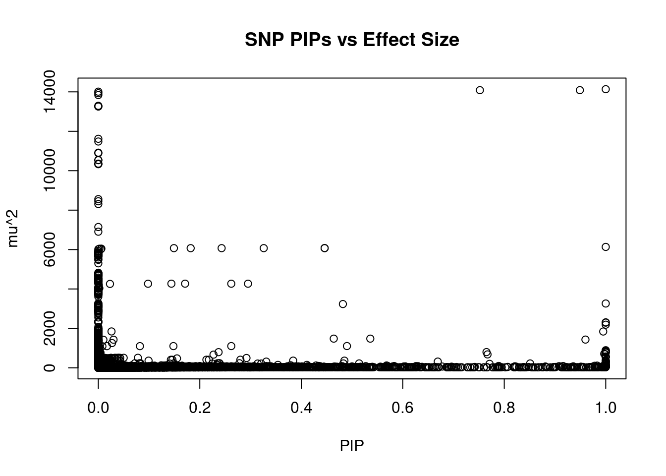
| Version | Author | Date |
|---|---|---|
| dfd2b5f | wesleycrouse | 2021-09-07 |
#SNPs with 50 largest effect sizes
head(ctwas_snp_res[order(-ctwas_snp_res$mu2),report_cols_snps],50)
id region_tag susie_pip mu2 PVE z
366007 rs199804242 6_89 1.000 14134.74 4.1e-02 4.09
366006 rs2327654 6_89 0.949 14086.90 3.9e-02 4.19
366023 rs6923513 6_89 0.752 14086.14 3.1e-02 4.17
366010 rs113527452 6_89 0.000 14011.37 7.9e-06 4.07
366015 rs200796875 6_89 0.000 13931.84 1.8e-07 4.13
366028 rs7756915 6_89 0.000 13839.49 1.4e-12 4.04
366021 rs6570040 6_89 0.000 13292.89 0.0e+00 4.36
366008 rs6570031 6_89 0.000 13262.82 0.0e+00 4.40
366009 rs9389323 6_89 0.000 13256.57 0.0e+00 4.34
366025 rs9321531 6_89 0.000 11619.25 0.0e+00 3.54
365998 rs9321528 6_89 0.000 11481.16 0.0e+00 3.97
366026 rs9494389 6_89 0.000 10915.42 0.0e+00 3.56
366030 rs5880262 6_89 0.000 10888.79 0.0e+00 3.39
366004 rs2208574 6_89 0.000 10541.49 0.0e+00 3.79
366003 rs1033755 6_89 0.000 10534.26 0.0e+00 3.56
366001 rs2038551 6_89 0.000 10358.54 0.0e+00 4.35
366012 rs9494377 6_89 0.000 10344.75 0.0e+00 3.60
365999 rs2038550 6_89 0.000 10330.45 0.0e+00 4.31
365988 rs6570026 6_89 0.000 8557.94 0.0e+00 3.38
365984 rs6926161 6_89 0.000 8449.45 0.0e+00 3.40
365993 rs6930773 6_89 0.000 8308.97 0.0e+00 3.94
365980 rs6925959 6_89 0.000 7143.44 0.0e+00 2.94
365985 rs6917005 6_89 0.000 6906.50 0.0e+00 3.09
1010181 rs202143810 20_38 1.000 6133.64 1.8e-02 -5.38
1010178 rs6089961 20_38 0.446 6073.77 7.9e-03 -5.48
1010180 rs2738758 20_38 0.446 6073.77 7.9e-03 -5.48
1010161 rs2750483 20_38 0.326 6072.06 5.8e-03 -5.48
1010159 rs35201382 20_38 0.149 6071.52 2.6e-03 -5.46
1010160 rs67468102 20_38 0.243 6071.17 4.3e-03 -5.48
1010156 rs2315009 20_38 0.182 6070.07 3.2e-03 -5.47
1010165 rs2259858 20_38 0.006 6045.77 9.8e-05 -5.47
1010158 rs35046559 20_38 0.002 6041.75 3.6e-05 -5.46
1010157 rs547768273 20_38 0.005 6016.49 8.6e-05 -5.54
1010177 rs145835311 20_38 0.000 6015.06 2.7e-06 -5.36
365981 rs6570023 6_89 0.000 5924.70 0.0e+00 2.95
365982 rs56976899 6_89 0.000 5917.94 0.0e+00 2.85
1010193 rs201555224 20_38 0.000 5838.78 9.4e-17 5.50
1010208 rs34251386 20_38 0.000 5836.34 3.0e-17 -5.48
1010183 rs2263805 20_38 0.000 5835.72 1.5e-17 -5.45
1010213 rs2427529 20_38 0.000 5835.67 3.2e-17 -5.48
1010204 rs1758205 20_38 0.000 5834.88 1.5e-17 -5.46
1010205 rs2263806 20_38 0.000 5834.37 7.5e-17 -5.47
1010153 rs2750482 20_38 0.000 5832.22 7.5e-18 -5.46
1010152 rs2750481 20_38 0.000 5832.20 7.5e-18 -5.46
1010150 rs2872881 20_38 0.000 5832.16 7.5e-18 -5.46
1010148 rs2750480 20_38 0.000 5830.30 3.8e-18 -5.45
1010239 rs2427534 20_38 0.000 5830.10 7.5e-18 -5.45
1010237 rs1151622 20_38 0.000 5829.66 1.1e-17 -5.47
1010212 rs6122154 20_38 0.000 5829.32 1.9e-17 -5.49
1010226 rs71325464 20_38 0.000 5829.08 3.8e-18 -5.45SNPs with highest PVE
#SNPs with 50 highest pve
head(ctwas_snp_res[order(-ctwas_snp_res$PVE),report_cols_snps],50)
id region_tag susie_pip mu2 PVE z
366007 rs199804242 6_89 1.000 14134.74 0.04100 4.09
366006 rs2327654 6_89 0.949 14086.90 0.03900 4.19
366023 rs6923513 6_89 0.752 14086.14 0.03100 4.17
1010181 rs202143810 20_38 1.000 6133.64 0.01800 -5.38
36042 rs7551731 1_78 1.000 3262.96 0.00950 -68.36
1010178 rs6089961 20_38 0.446 6073.77 0.00790 -5.48
1010180 rs2738758 20_38 0.446 6073.77 0.00790 -5.48
805278 rs440446 19_32 1.000 2291.43 0.00670 -28.59
805281 rs814573 19_32 1.000 2308.17 0.00670 -73.69
805277 rs405509 19_32 1.000 2189.10 0.00640 19.05
1010161 rs2750483 20_38 0.326 6072.06 0.00580 -5.48
635438 rs2393775 12_74 0.995 1841.42 0.00530 59.51
36035 rs2808628 1_78 0.482 3236.10 0.00450 -68.11
1010160 rs67468102 20_38 0.243 6071.17 0.00430 -5.48
17413 rs200241668 1_41 0.960 1432.90 0.00400 -50.44
1010176 rs6062504 20_38 0.295 4267.89 0.00370 9.60
1010174 rs4809328 20_38 0.262 4267.63 0.00330 9.59
1010156 rs2315009 20_38 0.182 6070.07 0.00320 -5.47
635435 rs1169286 12_74 1.000 893.52 0.00260 -46.10
1010159 rs35201382 20_38 0.149 6071.52 0.00260 -5.46
403738 rs761767938 7_49 1.000 870.09 0.00250 1.70
403746 rs1544459 7_49 1.000 850.58 0.00250 2.10
51446 rs78270913 1_106 1.000 822.28 0.00240 -2.05
89076 rs550064763 2_47 1.000 810.30 0.00240 -1.38
36037 rs2794521 1_78 0.536 1480.76 0.00230 3.73
51464 rs61820396 1_106 1.000 783.63 0.00230 -2.65
733175 rs17616063 16_27 1.000 766.81 0.00220 -27.92
36040 rs77289344 1_78 0.997 710.68 0.00210 42.02
1010175 rs4809329 20_38 0.171 4269.65 0.00210 9.56
36043 rs3116652 1_78 0.464 1481.15 0.00200 3.70
635450 rs2258043 12_74 0.999 688.68 0.00200 -40.50
89088 rs630241 2_47 0.765 798.63 0.00180 -2.19
1010179 rs4809330 20_38 0.144 4269.12 0.00180 9.54
17358 rs11811946 1_41 1.000 574.51 0.00170 32.07
89068 rs6737957 2_47 1.000 559.91 0.00160 -4.51
805272 rs116881820 19_32 1.000 547.46 0.00160 -30.35
868199 rs12133641 1_75 0.490 1104.72 0.00160 -38.83
873461 rs1260326 2_16 1.000 552.68 0.00160 -30.27
403735 rs10277379 7_49 0.767 680.66 0.00150 2.88
1010154 rs2315007 20_38 0.098 4265.91 0.00120 9.55
73863 rs569546056 2_17 1.000 379.07 0.00110 -2.15
433349 rs758184196 8_11 1.000 354.98 0.00100 -2.22
36004 rs12036827 1_78 1.000 320.85 0.00093 6.61
433323 rs1703982 8_11 1.000 316.69 0.00092 -7.50
868071 rs12083537 1_75 1.000 294.86 0.00086 -22.86
868193 rs12126142 1_75 0.262 1103.05 0.00084 -38.80
733093 rs62039688 16_27 1.000 259.87 0.00076 -15.21
133474 rs142215640 2_136 1.000 220.21 0.00064 3.76
433361 rs6993494 8_11 0.669 316.87 0.00062 5.99
64190 rs12239046 1_131 1.000 195.36 0.00057 16.09SNPs with largest z scores
#SNPs with 50 largest z scores
head(ctwas_snp_res[order(-abs(ctwas_snp_res$z)),report_cols_snps],50)
id region_tag susie_pip mu2 PVE z
805281 rs814573 19_32 1.000 2308.17 6.7e-03 -73.69
36042 rs7551731 1_78 1.000 3262.96 9.5e-03 -68.36
36035 rs2808628 1_78 0.482 3236.10 4.5e-03 -68.11
635438 rs2393775 12_74 0.995 1841.42 5.3e-03 59.51
635437 rs7979478 12_74 0.026 1845.54 1.4e-04 59.29
635448 rs1169311 12_74 0.001 1381.93 3.0e-06 -53.81
635425 rs2701194 12_74 0.027 1257.28 9.8e-05 50.78
635444 rs1169300 12_74 0.000 1129.25 9.6e-07 -50.74
17413 rs200241668 1_41 0.960 1432.90 4.0e-03 -50.44
17423 rs13375019 1_41 0.030 1426.27 1.3e-04 -50.37
17428 rs10789193 1_41 0.010 1423.53 4.0e-05 -50.34
17409 rs11208691 1_41 0.000 1408.54 5.1e-08 -50.15
36038 rs3116635 1_78 0.000 1041.09 0.0e+00 49.99
36044 rs12727021 1_78 0.000 1037.53 0.0e+00 49.98
17405 rs4655743 1_41 0.000 1366.36 1.1e-10 -49.67
17414 rs57274629 1_41 0.000 1418.23 6.2e-08 -49.50
17439 rs4655582 1_41 0.000 1333.27 2.5e-10 -49.01
17416 rs6697515 1_41 0.000 1319.85 4.4e-10 -48.34
17450 rs7515766 1_41 0.000 1252.40 5.8e-11 48.22
17452 rs7541434 1_41 0.000 1247.94 4.9e-11 48.18
635452 rs2258287 12_74 0.000 934.30 3.5e-07 -47.17
635435 rs1169286 12_74 1.000 893.52 2.6e-03 -46.10
36040 rs77289344 1_78 0.997 710.68 2.1e-03 42.02
36036 rs16842559 1_78 0.002 704.67 4.4e-06 41.86
36033 rs79162334 1_78 0.001 704.00 1.5e-06 41.69
36031 rs16842502 1_78 0.000 697.45 2.0e-07 41.60
635450 rs2258043 12_74 0.999 688.68 2.0e-03 -40.50
36046 rs12760041 1_78 0.000 453.43 0.0e+00 39.55
36045 rs12077166 1_78 0.000 605.18 0.0e+00 38.88
868199 rs12133641 1_75 0.490 1104.72 1.6e-03 -38.83
868193 rs12126142 1_75 0.262 1103.05 8.4e-04 -38.80
868177 rs61812598 1_75 0.148 1102.00 4.7e-04 -38.78
868196 rs4129267 1_75 0.082 1100.11 2.6e-04 -38.77
868175 rs12730935 1_75 0.017 1099.36 5.6e-05 -38.74
868198 rs2228145 1_75 0.008 1094.82 2.6e-05 -38.69
36047 rs11265266 1_78 0.000 480.57 0.0e+00 38.50
635417 rs7969196 12_74 0.001 701.23 1.5e-06 -38.32
868179 rs7512646 1_75 0.002 1070.33 4.9e-06 -38.25
868180 rs7529229 1_75 0.002 1070.34 4.9e-06 -38.25
868183 rs12404936 1_75 0.001 1065.47 4.1e-06 -38.18
635461 rs2859398 12_74 0.000 656.22 6.1e-07 -38.17
868182 rs12403159 1_75 0.001 1065.39 4.1e-06 -38.17
868169 rs4576655 1_75 0.001 1057.46 3.4e-06 -38.05
868170 rs4537545 1_75 0.001 1050.81 2.8e-06 -37.97
868168 rs11265613 1_75 0.001 1033.03 2.8e-06 -37.68
17435 rs55737039 1_41 0.000 499.37 1.6e-15 -37.67
17434 rs34618644 1_41 0.000 497.34 1.6e-15 -37.65
17443 rs6699885 1_41 0.000 494.69 1.6e-15 37.58
868159 rs12753254 1_75 0.001 1022.18 3.3e-06 -37.48
868160 rs12730036 1_75 0.001 1021.90 3.3e-06 -37.48Gene set enrichment for genes with PIP>0.8
#GO enrichment analysis
library(enrichR)
Welcome to enrichR
Checking connection ... Enrichr ... Connection is Live!
FlyEnrichr ... Connection is available!
WormEnrichr ... Connection is available!
YeastEnrichr ... Connection is available!
FishEnrichr ... Connection is available!dbs <- c("GO_Biological_Process_2021", "GO_Cellular_Component_2021", "GO_Molecular_Function_2021")
genes <- ctwas_gene_res$genename[ctwas_gene_res$susie_pip>0.8]
#number of genes for gene set enrichment
length(genes)[1] 20if (length(genes)>0){
GO_enrichment <- enrichr(genes, dbs)
for (db in dbs){
print(db)
df <- GO_enrichment[[db]]
df <- df[df$Adjusted.P.value<0.05,c("Term", "Overlap", "Adjusted.P.value", "Genes")]
print(df)
}
#DisGeNET enrichment
# devtools::install_bitbucket("ibi_group/disgenet2r")
library(disgenet2r)
disgenet_api_key <- get_disgenet_api_key(
email = "wesleycrouse@gmail.com",
password = "uchicago1" )
Sys.setenv(DISGENET_API_KEY= disgenet_api_key)
res_enrich <-disease_enrichment(entities=genes, vocabulary = "HGNC",
database = "CURATED" )
df <- res_enrich@qresult[1:10, c("Description", "FDR", "Ratio", "BgRatio")]
print(df)
#WebGestalt enrichment
library(WebGestaltR)
background <- ctwas_gene_res$genename
#listGeneSet()
databases <- c("pathway_KEGG", "disease_GLAD4U", "disease_OMIM")
enrichResult <- WebGestaltR(enrichMethod="ORA", organism="hsapiens",
interestGene=genes, referenceGene=background,
enrichDatabase=databases, interestGeneType="genesymbol",
referenceGeneType="genesymbol", isOutput=F)
print(enrichResult[,c("description", "size", "overlap", "FDR", "database", "userId")])
}Uploading data to Enrichr... Done.
Querying GO_Biological_Process_2021... Done.
Querying GO_Cellular_Component_2021... Done.
Querying GO_Molecular_Function_2021... Done.
Parsing results... Done.
[1] "GO_Biological_Process_2021"
[1] Term Overlap Adjusted.P.value Genes
<0 rows> (or 0-length row.names)
[1] "GO_Cellular_Component_2021"
[1] Term Overlap Adjusted.P.value Genes
<0 rows> (or 0-length row.names)
[1] "GO_Molecular_Function_2021"
[1] Term Overlap Adjusted.P.value Genes
<0 rows> (or 0-length row.names)RP11-219B17.3 gene(s) from the input list not found in DisGeNET CURATEDSNX17 gene(s) from the input list not found in DisGeNET CURATEDZNF793 gene(s) from the input list not found in DisGeNET CURATEDC10orf76 gene(s) from the input list not found in DisGeNET CURATEDKCNJ12 gene(s) from the input list not found in DisGeNET CURATEDRP11-806H10.4 gene(s) from the input list not found in DisGeNET CURATED Description
35 Opisthorchiasis
52 Carcinoma, Large Cell
64 Opisthorchis felineus Infection
65 Opisthorchis viverrini Infection
68 Fibrolamellar Hepatocellular Carcinoma
92 AICARDI-GOUTIERES SYNDROME 3
100 Alcohol Toxicity
112 MEGALENCEPHALY-POLYMICROGYRIA-POLYDACTYLY-HYDROCEPHALUS SYNDROME 3
113 PEELING SKIN SYNDROME 3
118 PEELING SKIN SYNDROME 6
FDR Ratio BgRatio
35 0.03403202 1/14 1/9703
52 0.03403202 1/14 2/9703
64 0.03403202 1/14 1/9703
65 0.03403202 1/14 1/9703
68 0.03403202 1/14 2/9703
92 0.03403202 1/14 1/9703
100 0.03403202 1/14 2/9703
112 0.03403202 1/14 1/9703
113 0.03403202 1/14 2/9703
118 0.03403202 1/14 2/9703******************************************
* *
* Welcome to WebGestaltR ! *
* *
******************************************Loading the functional categories...
Loading the ID list...
Loading the reference list...
Performing the enrichment analysis...Warning in oraEnrichment(interestGeneList, referenceGeneList, geneSet,
minNum = minNum, : No significant gene set is identified based on FDR 0.05!NULL
sessionInfo()R version 3.6.1 (2019-07-05)
Platform: x86_64-pc-linux-gnu (64-bit)
Running under: Scientific Linux 7.4 (Nitrogen)
Matrix products: default
BLAS/LAPACK: /software/openblas-0.2.19-el7-x86_64/lib/libopenblas_haswellp-r0.2.19.so
locale:
[1] LC_CTYPE=en_US.UTF-8 LC_NUMERIC=C
[3] LC_TIME=en_US.UTF-8 LC_COLLATE=en_US.UTF-8
[5] LC_MONETARY=en_US.UTF-8 LC_MESSAGES=en_US.UTF-8
[7] LC_PAPER=en_US.UTF-8 LC_NAME=C
[9] LC_ADDRESS=C LC_TELEPHONE=C
[11] LC_MEASUREMENT=en_US.UTF-8 LC_IDENTIFICATION=C
attached base packages:
[1] stats graphics grDevices utils datasets methods base
other attached packages:
[1] WebGestaltR_0.4.4 disgenet2r_0.99.2 enrichR_3.0 cowplot_1.0.0
[5] ggplot2_3.3.3
loaded via a namespace (and not attached):
[1] bitops_1.0-6 matrixStats_0.57.0
[3] fs_1.3.1 bit64_4.0.5
[5] doParallel_1.0.16 progress_1.2.2
[7] httr_1.4.1 rprojroot_2.0.2
[9] GenomeInfoDb_1.20.0 doRNG_1.8.2
[11] tools_3.6.1 utf8_1.2.1
[13] R6_2.5.0 DBI_1.1.1
[15] BiocGenerics_0.30.0 colorspace_1.4-1
[17] withr_2.4.1 tidyselect_1.1.0
[19] prettyunits_1.0.2 bit_4.0.4
[21] curl_3.3 compiler_3.6.1
[23] git2r_0.26.1 Biobase_2.44.0
[25] DelayedArray_0.10.0 rtracklayer_1.44.0
[27] labeling_0.3 scales_1.1.0
[29] readr_1.4.0 apcluster_1.4.8
[31] stringr_1.4.0 digest_0.6.20
[33] Rsamtools_2.0.0 svglite_1.2.2
[35] rmarkdown_1.13 XVector_0.24.0
[37] pkgconfig_2.0.3 htmltools_0.3.6
[39] fastmap_1.1.0 BSgenome_1.52.0
[41] rlang_0.4.11 RSQLite_2.2.7
[43] generics_0.0.2 farver_2.1.0
[45] jsonlite_1.6 BiocParallel_1.18.0
[47] dplyr_1.0.7 VariantAnnotation_1.30.1
[49] RCurl_1.98-1.1 magrittr_2.0.1
[51] GenomeInfoDbData_1.2.1 Matrix_1.2-18
[53] Rcpp_1.0.6 munsell_0.5.0
[55] S4Vectors_0.22.1 fansi_0.5.0
[57] gdtools_0.1.9 lifecycle_1.0.0
[59] stringi_1.4.3 whisker_0.3-2
[61] yaml_2.2.0 SummarizedExperiment_1.14.1
[63] zlibbioc_1.30.0 plyr_1.8.4
[65] grid_3.6.1 blob_1.2.1
[67] parallel_3.6.1 promises_1.0.1
[69] crayon_1.4.1 lattice_0.20-38
[71] Biostrings_2.52.0 GenomicFeatures_1.36.3
[73] hms_1.1.0 knitr_1.23
[75] pillar_1.6.1 igraph_1.2.4.1
[77] GenomicRanges_1.36.0 rjson_0.2.20
[79] rngtools_1.5 codetools_0.2-16
[81] reshape2_1.4.3 biomaRt_2.40.1
[83] stats4_3.6.1 XML_3.98-1.20
[85] glue_1.4.2 evaluate_0.14
[87] data.table_1.14.0 foreach_1.5.1
[89] vctrs_0.3.8 httpuv_1.5.1
[91] gtable_0.3.0 purrr_0.3.4
[93] assertthat_0.2.1 cachem_1.0.5
[95] xfun_0.8 later_0.8.0
[97] tibble_3.1.2 iterators_1.0.13
[99] GenomicAlignments_1.20.1 AnnotationDbi_1.46.0
[101] memoise_2.0.0 IRanges_2.18.1
[103] workflowr_1.6.2 ellipsis_0.3.2