Direct bilirubin (quantile) - Whole_Blood
wesleycrouse
2021-09-09
Last updated: 2021-09-09
Checks: 6 1
Knit directory: ctwas_applied/
This reproducible R Markdown analysis was created with workflowr (version 1.6.2). The Checks tab describes the reproducibility checks that were applied when the results were created. The Past versions tab lists the development history.
The R Markdown file has unstaged changes. To know which version of the R Markdown file created these results, you’ll want to first commit it to the Git repo. If you’re still working on the analysis, you can ignore this warning. When you’re finished, you can run wflow_publish to commit the R Markdown file and build the HTML.
Great job! The global environment was empty. Objects defined in the global environment can affect the analysis in your R Markdown file in unknown ways. For reproduciblity it’s best to always run the code in an empty environment.
The command set.seed(20210726) was run prior to running the code in the R Markdown file. Setting a seed ensures that any results that rely on randomness, e.g. subsampling or permutations, are reproducible.
Great job! Recording the operating system, R version, and package versions is critical for reproducibility.
Nice! There were no cached chunks for this analysis, so you can be confident that you successfully produced the results during this run.
Great job! Using relative paths to the files within your workflowr project makes it easier to run your code on other machines.
Great! You are using Git for version control. Tracking code development and connecting the code version to the results is critical for reproducibility.
The results in this page were generated with repository version 59e5f4d. See the Past versions tab to see a history of the changes made to the R Markdown and HTML files.
Note that you need to be careful to ensure that all relevant files for the analysis have been committed to Git prior to generating the results (you can use wflow_publish or wflow_git_commit). workflowr only checks the R Markdown file, but you know if there are other scripts or data files that it depends on. Below is the status of the Git repository when the results were generated:
Unstaged changes:
    Modified:   analysis/ukb-d-30500_irnt_Liver.Rmd
    Modified:   analysis/ukb-d-30500_irnt_Whole_Blood.Rmd
    Modified:   analysis/ukb-d-30600_irnt_Liver.Rmd
    Modified:   analysis/ukb-d-30600_irnt_Whole_Blood.Rmd
    Modified:   analysis/ukb-d-30610_irnt_Liver.Rmd
    Modified:   analysis/ukb-d-30610_irnt_Whole_Blood.Rmd
    Modified:   analysis/ukb-d-30620_irnt_Liver.Rmd
    Modified:   analysis/ukb-d-30620_irnt_Whole_Blood.Rmd
    Modified:   analysis/ukb-d-30630_irnt_Liver.Rmd
    Modified:   analysis/ukb-d-30630_irnt_Whole_Blood.Rmd
    Modified:   analysis/ukb-d-30640_irnt_Liver.Rmd
    Modified:   analysis/ukb-d-30640_irnt_Whole_Blood.Rmd
    Modified:   analysis/ukb-d-30650_irnt_Liver.Rmd
    Modified:   analysis/ukb-d-30650_irnt_Whole_Blood.Rmd
    Modified:   analysis/ukb-d-30660_irnt_Liver.Rmd
    Modified:   analysis/ukb-d-30660_irnt_Whole_Blood.Rmd
    Modified:   analysis/ukb-d-30670_irnt_Liver.Rmd
    Modified:   analysis/ukb-d-30680_irnt_Liver.Rmd
    Modified:   analysis/ukb-d-30690_irnt_Liver.Rmd
    Modified:   analysis/ukb-d-30700_irnt_Liver.Rmd
    Modified:   analysis/ukb-d-30710_irnt_Liver.Rmd
    Modified:   analysis/ukb-d-30720_irnt_Liver.Rmd
    Modified:   analysis/ukb-d-30730_irnt_Liver.Rmd
    Modified:   analysis/ukb-d-30740_irnt_Liver.Rmd
    Modified:   analysis/ukb-d-30750_irnt_Liver.Rmd
    Modified:   analysis/ukb-d-30760_irnt_Liver.Rmd
    Modified:   analysis/ukb-d-30770_irnt_Liver.Rmd
    Modified:   analysis/ukb-d-30780_irnt_Liver.Rmd
    Modified:   analysis/ukb-d-30790_irnt_Liver.Rmd
    Modified:   analysis/ukb-d-30800_irnt_Liver.Rmd
    Modified:   analysis/ukb-d-30810_irnt_Liver.Rmd
    Modified:   analysis/ukb-d-30820_irnt_Liver.Rmd
    Modified:   analysis/ukb-d-30830_irnt_Liver.Rmd
    Modified:   analysis/ukb-d-30840_irnt_Liver.Rmd
    Modified:   analysis/ukb-d-30850_irnt_Liver.Rmd
    Modified:   analysis/ukb-d-30860_irnt_Liver.Rmd
    Modified:   analysis/ukb-d-30870_irnt_Liver.Rmd
    Modified:   analysis/ukb-d-30880_irnt_Liver.Rmd
    Modified:   analysis/ukb-d-30890_irnt_Liver.Rmd
Note that any generated files, e.g. HTML, png, CSS, etc., are not included in this status report because it is ok for generated content to have uncommitted changes.
These are the previous versions of the repository in which changes were made to the R Markdown (analysis/ukb-d-30660_irnt_Whole_Blood.Rmd) and HTML (docs/ukb-d-30660_irnt_Whole_Blood.html) files. If you’ve configured a remote Git repository (see ?wflow_git_remote), click on the hyperlinks in the table below to view the files as they were in that past version.
| File | Version | Author | Date | Message |
|---|---|---|---|---|
| Rmd | cbf7408 | wesleycrouse | 2021-09-08 | adding enrichment to reports |
| html | cbf7408 | wesleycrouse | 2021-09-08 | adding enrichment to reports |
| Rmd | 4970e3e | wesleycrouse | 2021-09-08 | updating reports |
| html | 4970e3e | wesleycrouse | 2021-09-08 | updating reports |
| Rmd | dfd2b5f | wesleycrouse | 2021-09-07 | regenerating reports |
| html | dfd2b5f | wesleycrouse | 2021-09-07 | regenerating reports |
| Rmd | 61b53b3 | wesleycrouse | 2021-09-06 | updated PVE calculation |
| html | 61b53b3 | wesleycrouse | 2021-09-06 | updated PVE calculation |
| Rmd | 837dd01 | wesleycrouse | 2021-09-01 | adding additional fixedsigma report |
| Rmd | d0a5417 | wesleycrouse | 2021-08-30 | adding new reports to the index |
| Rmd | 0922de7 | wesleycrouse | 2021-08-18 | updating all reports with locus plots |
| html | 0922de7 | wesleycrouse | 2021-08-18 | updating all reports with locus plots |
| html | 1c62980 | wesleycrouse | 2021-08-11 | Updating reports |
| Rmd | 5981e80 | wesleycrouse | 2021-08-11 | Adding more reports |
| html | 5981e80 | wesleycrouse | 2021-08-11 | Adding more reports |
| Rmd | da9f015 | wesleycrouse | 2021-08-07 | adding more reports |
| html | da9f015 | wesleycrouse | 2021-08-07 | adding more reports |
Overview
These are the results of a ctwas analysis of the UK Biobank trait Direct bilirubin (quantile) using Whole_Blood gene weights.
The GWAS was conducted by the Neale Lab, and the biomarker traits we analyzed are discussed here. Summary statistics were obtained from IEU OpenGWAS using GWAS ID: ukb-d-30660_irnt. Results were obtained from from IEU rather than Neale Lab because they are in a standardard format (GWAS VCF). Note that 3 of the 34 biomarker traits were not available from IEU and were excluded from analysis.
The weights are mashr GTEx v8 models on Whole_Blood eQTL obtained from PredictDB. We performed a full harmonization of the variants, including recovering strand ambiguous variants. This procedure is discussed in a separate document. (TO-DO: add report that describes harmonization)
LD matrices were computed from a 10% subset of Neale lab subjects. Subjects were matched using the plate and well information from genotyping. We included only biallelic variants with MAF>0.01 in the original Neale Lab GWAS. (TO-DO: add more details [number of subjects, variants, etc])
Weight QC
TO-DO: add enhanced QC reporting (total number of weights, why each variant was missing for all genes)
qclist_all <- list()

qc_files <- paste0(results_dir, "/", list.files(results_dir, pattern="exprqc.Rd"))

for (i in 1:length(qc_files)){
  load(qc_files[i])
  chr <- unlist(strsplit(rev(unlist(strsplit(qc_files[i], "_")))[1], "[.]"))[1]
  qclist_all[[chr]] <- cbind(do.call(rbind, lapply(qclist,unlist)), as.numeric(substring(chr,4)))
}

qclist_all <- data.frame(do.call(rbind, qclist_all))
colnames(qclist_all)[ncol(qclist_all)] <- "chr"

rm(qclist, wgtlist, z_gene_chr)

#number of imputed weights
nrow(qclist_all)
[1] 11095#number of imputed weights by chromosome
table(qclist_all$chr)
   1    2    3    4    5    6    7    8    9   10   11   12   13   14   15
1129  747  624  400  479  621  560  383  404  430  682  652  192  362  331
  16   17   18   19   20   21   22
 551  725  159  911  313  130  310
#proportion of imputed weights without missing variants
mean(qclist_all$nmiss==0)[1] 0.762776Load ctwas results
#load ctwas results
ctwas_res <- data.table::fread(paste0(results_dir, "/", analysis_id, "_ctwas.susieIrss.txt"))

#make unique identifier for regions
ctwas_res$region_tag <- paste(ctwas_res$region_tag1, ctwas_res$region_tag2, sep="_")

#compute PVE for each gene/SNP
ctwas_res$PVE = ctwas_res$susie_pip*ctwas_res$mu2/sample_size #check PVE calculation

#separate gene and SNP results
ctwas_gene_res <- ctwas_res[ctwas_res$type == "gene", ]
ctwas_gene_res <- data.frame(ctwas_gene_res)
ctwas_snp_res <- ctwas_res[ctwas_res$type == "SNP", ]
ctwas_snp_res <- data.frame(ctwas_snp_res)

#add gene information to results
sqlite <- RSQLite::dbDriver("SQLite")
db = RSQLite::dbConnect(sqlite, paste0("/project2/compbio/predictdb/mashr_models/mashr_", weight, ".db"))
query <- function(...) RSQLite::dbGetQuery(db, ...)
gene_info <- query("select gene, genename from extra")
gene_info <- query("select gene, genename, gene_type from extra")
RSQLite::dbDisconnect(db)

ctwas_gene_res <- cbind(ctwas_gene_res, gene_info[sapply(ctwas_gene_res$id, match, gene_info$gene), c("genename", "gene_type")])

#add z score to results
load(paste0(results_dir, "/", analysis_id, "_expr_z_gene.Rd"))
ctwas_gene_res$z <- z_gene[ctwas_gene_res$id,]$z

#load(paste0(results_dir, "/", analysis_id, "_expr_z_snp.Rd")) #for new version, stored after harmonization
z_snp <- readRDS(paste0(results_dir, "/", trait_id, ".RDS")) #for old version, unharmonized

z_snp <- z_snp[z_snp$id %in% ctwas_snp_res$id,] #subset snps to those included in analysis, note some are duplicated, need to match which allele was used
ctwas_snp_res$z <- z_snp$z[match(ctwas_snp_res$id, z_snp$id)] #for duplicated snps, this arbitrarily uses the first allele
ctwas_snp_res$z_flag <- as.numeric(ctwas_snp_res$id %in% z_snp$id[duplicated(z_snp$id)]) #mark the unclear z scores, flag=1

#formatting and rounding for tables
ctwas_gene_res$z <- round(ctwas_gene_res$z,2)
ctwas_snp_res$z <- round(ctwas_snp_res$z,2)
ctwas_gene_res$susie_pip <- round(ctwas_gene_res$susie_pip,3)
ctwas_snp_res$susie_pip <- round(ctwas_snp_res$susie_pip,3)
ctwas_gene_res$mu2 <- round(ctwas_gene_res$mu2,2)
ctwas_snp_res$mu2 <- round(ctwas_snp_res$mu2,2)
ctwas_gene_res$PVE <- signif(ctwas_gene_res$PVE, 2)
ctwas_snp_res$PVE <- signif(ctwas_snp_res$PVE, 2)

#merge gene and snp results with added information
ctwas_gene_res$z_flag=NA
ctwas_snp_res$genename=NA
ctwas_snp_res$gene_type=NA

ctwas_res <- rbind(ctwas_gene_res,
                   ctwas_snp_res[,colnames(ctwas_gene_res)])

#store columns to report
report_cols <- colnames(ctwas_gene_res)[!(colnames(ctwas_gene_res) %in% c("type", "region_tag1", "region_tag2", "cs_index", "gene_type", "z_flag", "id", "chrom", "pos"))]
first_cols <- c("genename", "region_tag")
report_cols <- c(first_cols, report_cols[!(report_cols %in% first_cols)])

report_cols_snps <- c("id", report_cols[-1])

#get number of SNPs from s1 results; adjust for thin
ctwas_res_s1 <- data.table::fread(paste0(results_dir, "/", analysis_id, "_ctwas.s1.susieIrss.txt"))
n_snps <- sum(ctwas_res_s1$type=="SNP")/thin
rm(ctwas_res_s1)
Check convergence of parameters
library(ggplot2)
library(cowplot)
********************************************************Note: As of version 1.0.0, cowplot does not change the default ggplot2 theme anymore. To recover the previous behavior, execute:
theme_set(theme_cowplot())********************************************************load(paste0(results_dir, "/", analysis_id, "_ctwas.s2.susieIrssres.Rd"))
df <- data.frame(niter = rep(1:ncol(group_prior_rec), 2),
value = c(group_prior_rec[1,], group_prior_rec[2,]),
group = rep(c("Gene", "SNP"), each = ncol(group_prior_rec)))
df$group <- as.factor(df$group)
df$value[df$group=="SNP"] <- df$value[df$group=="SNP"]*thin #adjust parameter to account for thin argument
p_pi <- ggplot(df, aes(x=niter, y=value, group=group)) +
geom_line(aes(color=group)) +
geom_point(aes(color=group)) +
xlab("Iteration") + ylab(bquote(pi)) +
ggtitle("Prior mean") +
theme_cowplot()
df <- data.frame(niter = rep(1:ncol(group_prior_var_rec), 2),
value = c(group_prior_var_rec[1,], group_prior_var_rec[2,]),
group = rep(c("Gene", "SNP"), each = ncol(group_prior_var_rec)))
df$group <- as.factor(df$group)
p_sigma2 <- ggplot(df, aes(x=niter, y=value, group=group)) +
geom_line(aes(color=group)) +
geom_point(aes(color=group)) +
xlab("Iteration") + ylab(bquote(sigma^2)) +
ggtitle("Prior variance") +
theme_cowplot()
plot_grid(p_pi, p_sigma2)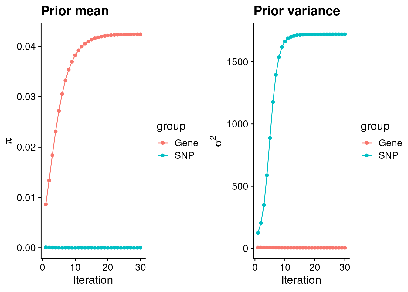
| Version | Author | Date |
|---|---|---|
| dfd2b5f | wesleycrouse | 2021-09-07 |
#estimated group prior
estimated_group_prior <- group_prior_rec[,ncol(group_prior_rec)]
names(estimated_group_prior) <- c("gene", "snp")
estimated_group_prior["snp"] <- estimated_group_prior["snp"]*thin #adjust parameter to account for thin argument
print(estimated_group_prior)
gene snp
4.239424e-02 6.079391e-06 #estimated group prior variance
estimated_group_prior_var <- group_prior_var_rec[,ncol(group_prior_var_rec)]
names(estimated_group_prior_var) <- c("gene", "snp")
print(estimated_group_prior_var) gene snp
5.602468 1721.238484 #report sample size
print(sample_size)[1] 292933#report group size
group_size <- c(nrow(ctwas_gene_res), n_snps)
print(group_size)[1] 11095 8697330#estimated group PVE
estimated_group_pve <- estimated_group_prior_var*estimated_group_prior*group_size/sample_size #check PVE calculation
names(estimated_group_pve) <- c("gene", "snp")
print(estimated_group_pve) gene snp
0.008995913 0.310683934 #compare sum(PIP*mu2/sample_size) with above PVE calculation
c(sum(ctwas_gene_res$PVE),sum(ctwas_snp_res$PVE))[1] 0.05365313 0.91115777Genes with highest PIPs
#distribution of PIPs
hist(ctwas_gene_res$susie_pip, xlim=c(0,1), main="Distribution of Gene PIPs")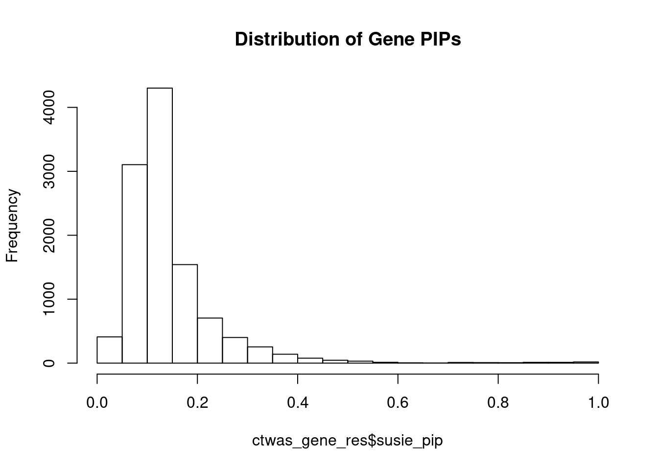
| Version | Author | Date |
|---|---|---|
| dfd2b5f | wesleycrouse | 2021-09-07 |
#genes with PIP>0.8 or 20 highest PIPs
head(ctwas_gene_res[order(-ctwas_gene_res$susie_pip),report_cols], max(sum(ctwas_gene_res$susie_pip>0.8), 20))
genename region_tag susie_pip mu2 PVE z
5318 USP3 15_29 0.998 29.74 1.0e-04 5.91
1267 PABPC4 1_24 0.993 21.32 7.2e-05 4.53
7189 ARHGAP25 2_45 0.993 20.90 7.1e-05 4.63
10164 RNFT1 17_35 0.992 30.82 1.0e-04 5.99
5880 PHIP 6_54 0.990 22.41 7.6e-05 4.84
5839 TIMD4 5_92 0.988 24.00 8.1e-05 -5.06
1181 DNMT3B 20_19 0.988 18.91 6.4e-05 -3.98
8978 SMIM19 8_37 0.984 28.00 9.4e-05 -5.58
7786 CATSPER2 15_16 0.980 18.95 6.3e-05 -4.43
8294 GYPA 4_94 0.969 20.41 6.8e-05 4.83
10508 ADH5 4_66 0.966 28.82 9.5e-05 5.62
6327 TXNDC11 16_12 0.965 17.58 5.8e-05 3.92
562 DGAT2 11_42 0.962 45.37 1.5e-04 -7.48
6076 ZC3H12C 11_65 0.961 18.07 5.9e-05 4.16
5207 SCAF11 12_29 0.960 17.81 5.8e-05 4.13
6181 CSNK1G3 5_75 0.958 18.85 6.2e-05 -4.30
5665 CNIH4 1_114 0.956 17.56 5.7e-05 -3.98
7258 ICA1L 2_120 0.952 23.67 7.7e-05 5.14
10805 EHMT2 6_26 0.946 36.51 1.2e-04 6.43
6290 ZFP36L2 2_27 0.945 17.47 5.6e-05 -3.79
4296 PDLIM4 5_79 0.932 18.08 5.8e-05 -4.33
12471 RP11-334C17.6 17_45 0.929 17.37 5.5e-05 4.06
7782 CASC4 15_17 0.928 16.88 5.3e-05 3.91
4559 GSTM1 1_67 0.926 17.51 5.5e-05 -4.22
4151 LDLR 19_9 0.925 17.52 5.5e-05 3.92
8291 SIK2 11_66 0.921 18.97 6.0e-05 4.45
9687 MROH7 1_34 0.920 16.70 5.2e-05 -3.86
4656 NREP 5_66 0.917 17.94 5.6e-05 -4.19
11446 RP11-9M16.2 9_59 0.912 17.15 5.3e-05 -3.97
12450 RP11-88E10.5 13_61 0.909 17.23 5.3e-05 3.90
1164 NID2 14_21 0.893 16.60 5.1e-05 3.79
9223 ZBTB7A 19_4 0.891 17.86 5.4e-05 3.91
10700 MAP3K3 17_37 0.886 16.19 4.9e-05 3.51
746 SMG6 17_3 0.882 17.18 5.2e-05 -4.05
7393 CEP44 4_113 0.881 17.00 5.1e-05 3.81
8098 NDUFS5 1_24 0.876 16.71 5.0e-05 3.53
10733 CENPW 6_84 0.875 16.87 5.0e-05 3.71
5268 CUL4A 13_62 0.875 17.51 5.2e-05 -4.04
2097 RASIP1 19_33 0.872 18.85 5.6e-05 4.10
4660 UBQLN1 9_41 0.869 16.99 5.0e-05 3.75
3848 RRBP1 20_13 0.862 17.56 5.2e-05 -4.08
1723 MAPRE1 20_19 0.851 16.10 4.7e-05 -3.23
7627 STOX1 10_46 0.840 15.69 4.5e-05 2.88
6552 HKDC1 10_46 0.835 22.43 6.4e-05 5.40
5692 ASXL2 2_15 0.825 16.69 4.7e-05 3.61
4398 UNK 17_42 0.815 26.16 7.3e-05 -5.28
2237 TBL2 7_47 0.814 17.07 4.7e-05 -3.63
8528 DRC3 17_15 0.814 16.96 4.7e-05 -3.77
7577 ZCCHC24 10_51 0.812 16.88 4.7e-05 3.60Genes with largest effect sizes
#plot PIP vs effect size
plot(ctwas_gene_res$susie_pip, ctwas_gene_res$mu2, xlab="PIP", ylab="mu^2", main="Gene PIPs vs Effect Size")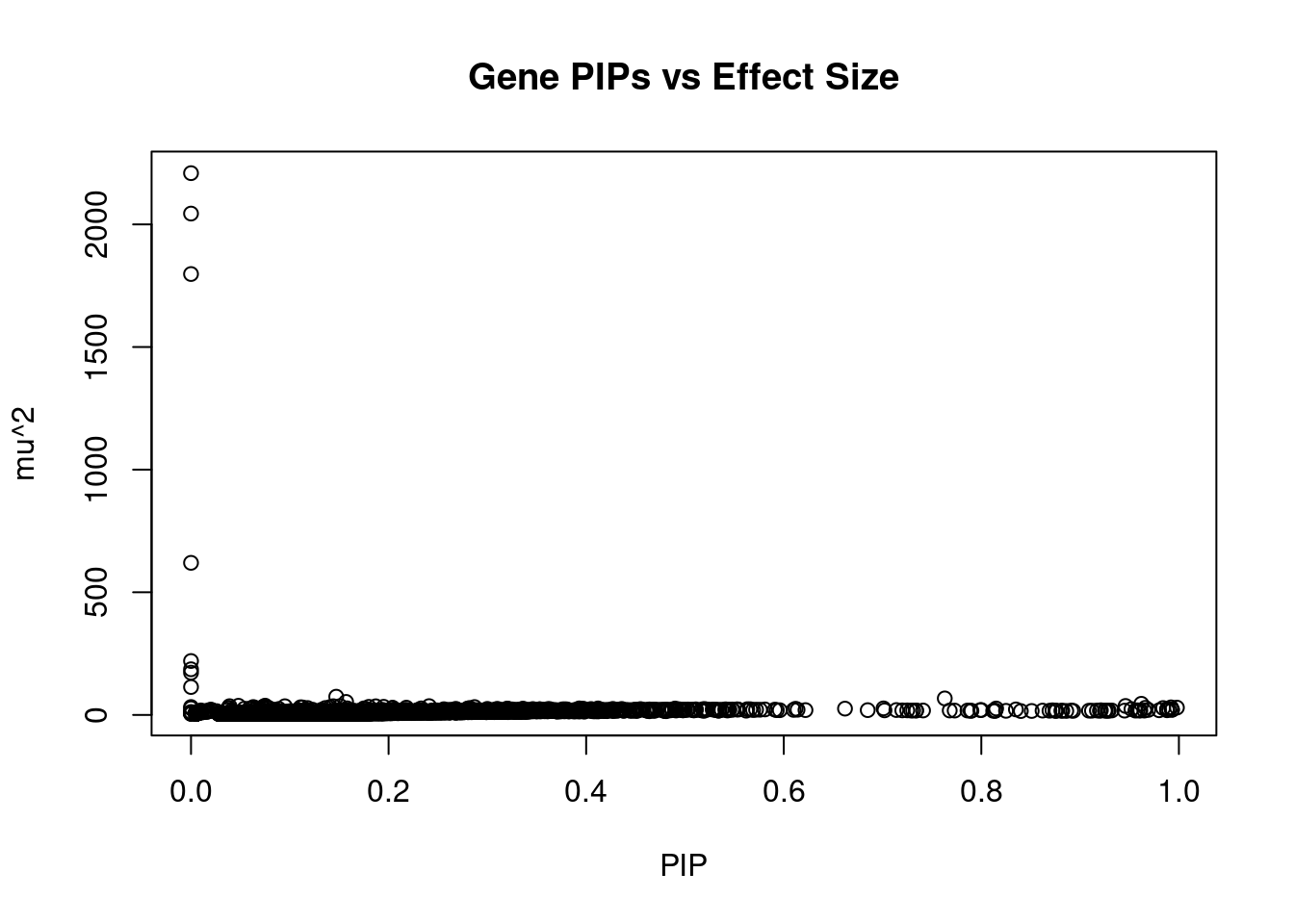
| Version | Author | Date |
|---|---|---|
| dfd2b5f | wesleycrouse | 2021-09-07 |
#genes with 20 largest effect sizes
head(ctwas_gene_res[order(-ctwas_gene_res$mu2),report_cols],20)
genename region_tag susie_pip mu2 PVE z
922 DGKD 2_137 0.000 2208.93 0.0e+00 -48.36
7255 EIF5A2 3_104 0.000 2044.10 3.0e-12 -4.10
1119 USP40 2_137 0.000 1797.68 0.0e+00 49.12
1118 ATG16L1 2_137 0.000 620.09 0.0e+00 -28.30
2657 GOLT1B 12_16 0.000 219.77 0.0e+00 -2.87
40 RECQL 12_16 0.000 186.05 0.0e+00 2.39
3636 HJURP 2_137 0.000 172.18 0.0e+00 10.96
4608 SPX 12_16 0.000 113.76 0.0e+00 2.04
4137 MAU2 19_15 0.147 74.30 3.7e-05 -9.61
7536 NFIL3 9_46 0.763 67.27 1.8e-04 9.30
2131 ATP13A1 19_15 0.157 53.03 2.8e-05 8.15
562 DGAT2 11_42 0.962 45.37 1.5e-04 -7.48
11441 APOC2 19_31 0.075 37.74 9.6e-06 -6.87
11048 DDAH2 6_26 0.048 37.32 6.1e-06 5.72
10805 EHMT2 6_26 0.946 36.51 1.2e-04 6.43
11433 MAPKAPK5-AS1 12_67 0.151 36.20 1.9e-05 -7.24
661 ZNRD1 6_26 0.241 35.77 2.9e-05 3.90
10608 HLA-DRB5 6_26 0.039 35.64 4.8e-06 5.67
4969 TCF19 6_26 0.144 35.47 1.7e-05 -4.54
5092 EXOC6 10_59 0.095 35.39 1.2e-05 -6.37Genes with highest PVE
#genes with 20 highest pve
head(ctwas_gene_res[order(-ctwas_gene_res$PVE),report_cols],20)
genename region_tag susie_pip mu2 PVE z
7536 NFIL3 9_46 0.763 67.27 1.8e-04 9.30
562 DGAT2 11_42 0.962 45.37 1.5e-04 -7.48
10805 EHMT2 6_26 0.946 36.51 1.2e-04 6.43
5318 USP3 15_29 0.998 29.74 1.0e-04 5.91
10164 RNFT1 17_35 0.992 30.82 1.0e-04 5.99
10508 ADH5 4_66 0.966 28.82 9.5e-05 5.62
8978 SMIM19 8_37 0.984 28.00 9.4e-05 -5.58
5839 TIMD4 5_92 0.988 24.00 8.1e-05 -5.06
7258 ICA1L 2_120 0.952 23.67 7.7e-05 5.14
5880 PHIP 6_54 0.990 22.41 7.6e-05 4.84
4398 UNK 17_42 0.815 26.16 7.3e-05 -5.28
1267 PABPC4 1_24 0.993 21.32 7.2e-05 4.53
7189 ARHGAP25 2_45 0.993 20.90 7.1e-05 4.63
8294 GYPA 4_94 0.969 20.41 6.8e-05 4.83
11755 RP11-452H21.4 11_43 0.701 26.62 6.4e-05 5.54
6552 HKDC1 10_46 0.835 22.43 6.4e-05 5.40
1181 DNMT3B 20_19 0.988 18.91 6.4e-05 -3.98
7786 CATSPER2 15_16 0.980 18.95 6.3e-05 -4.43
6181 CSNK1G3 5_75 0.958 18.85 6.2e-05 -4.30
8291 SIK2 11_66 0.921 18.97 6.0e-05 4.45Genes with largest z scores
#genes with 20 largest z scores
head(ctwas_gene_res[order(-abs(ctwas_gene_res$z)),report_cols],20)
genename region_tag susie_pip mu2 PVE z
1119 USP40 2_137 0.000 1797.68 0.0e+00 49.12
922 DGKD 2_137 0.000 2208.93 0.0e+00 -48.36
1118 ATG16L1 2_137 0.000 620.09 0.0e+00 -28.30
3636 HJURP 2_137 0.000 172.18 0.0e+00 10.96
4137 MAU2 19_15 0.147 74.30 3.7e-05 -9.61
7536 NFIL3 9_46 0.763 67.27 1.8e-04 9.30
2131 ATP13A1 19_15 0.157 53.03 2.8e-05 8.15
562 DGAT2 11_42 0.962 45.37 1.5e-04 -7.48
11433 MAPKAPK5-AS1 12_67 0.151 36.20 1.9e-05 -7.24
11441 APOC2 19_31 0.075 37.74 9.6e-06 -6.87
2607 SH2B3 12_67 0.077 29.85 7.8e-06 6.80
1366 CWF19L1 10_64 0.612 25.11 5.2e-05 -6.77
2220 AHR 7_17 0.059 25.30 5.1e-06 -6.58
10204 BLOC1S2 10_64 0.455 23.75 3.7e-05 -6.48
5979 AUH 9_46 0.076 33.32 8.6e-06 6.47
10805 EHMT2 6_26 0.946 36.51 1.2e-04 6.43
2611 ALDH2 12_67 0.187 35.19 2.2e-05 -6.42
5092 EXOC6 10_59 0.095 35.39 1.2e-05 -6.37
1210 MAPKAPK5 12_67 0.218 29.58 2.2e-05 6.30
1227 ERP29 12_67 0.204 28.77 2.0e-05 6.25Comparing z scores and PIPs
#set nominal signifiance threshold for z scores
alpha <- 0.05

#bonferroni adjusted threshold for z scores
sig_thresh <- qnorm(1-(alpha/nrow(ctwas_gene_res)/2), lower=T)

#Q-Q plot for z scores
obs_z <- ctwas_gene_res$z[order(ctwas_gene_res$z)]
exp_z <- qnorm((1:nrow(ctwas_gene_res))/nrow(ctwas_gene_res))

plot(exp_z, obs_z, xlab="Expected z", ylab="Observed z", main="Gene z score Q-Q plot")
abline(a=0,b=1)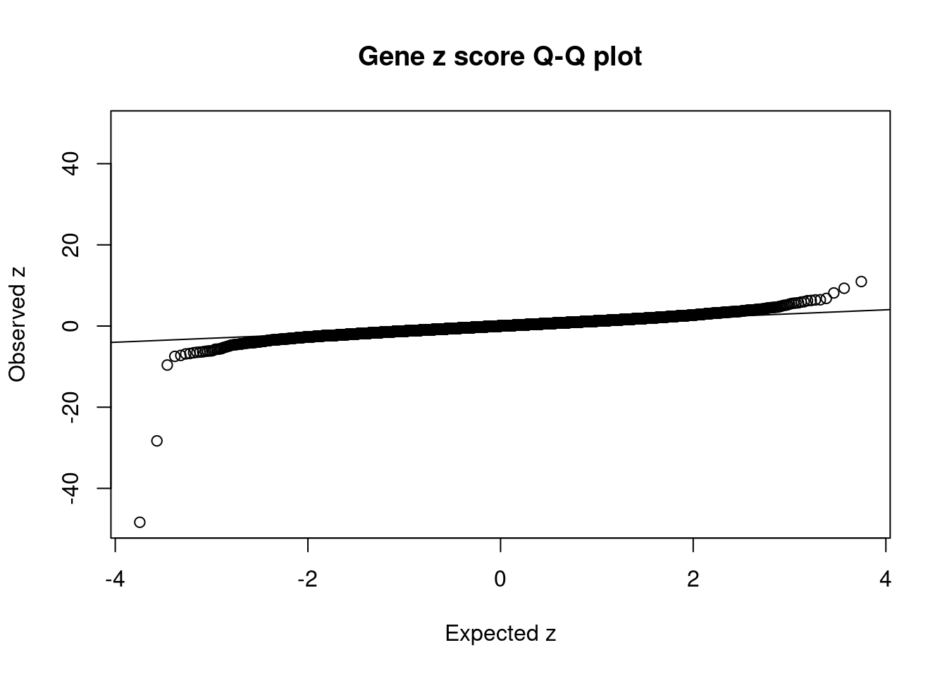
| Version | Author | Date |
|---|---|---|
| dfd2b5f | wesleycrouse | 2021-09-07 |
#plot z score vs PIP
plot(abs(ctwas_gene_res$z), ctwas_gene_res$susie_pip, xlab="abs(z)", ylab="PIP")
abline(v=sig_thresh, col="red", lty=2)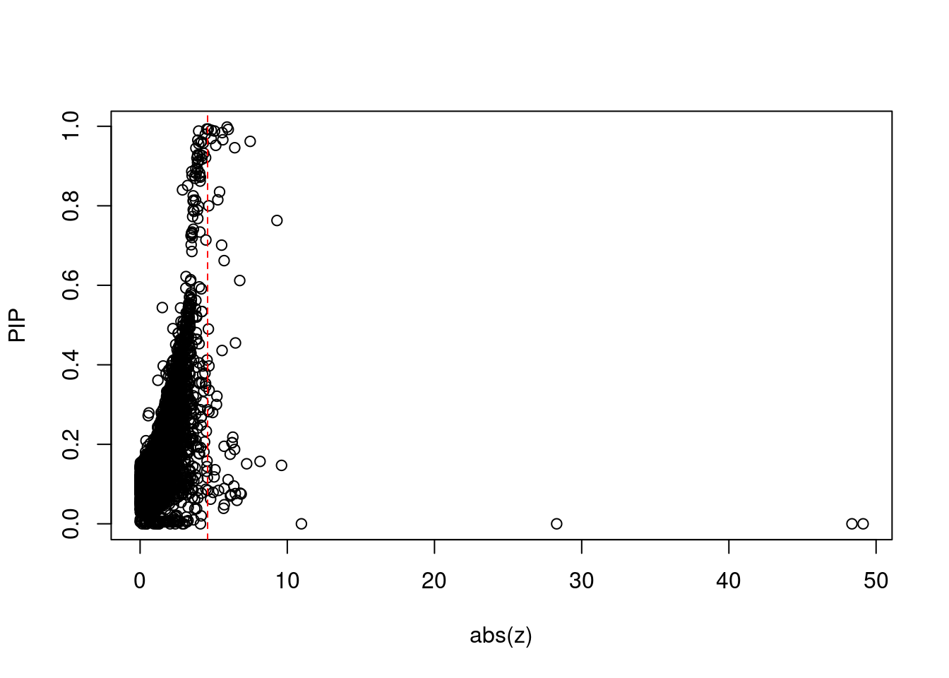
| Version | Author | Date |
|---|---|---|
| dfd2b5f | wesleycrouse | 2021-09-07 |
#proportion of significant z scores
mean(abs(ctwas_gene_res$z) > sig_thresh)
[1] 0.00522758#genes with most significant z scores
head(ctwas_gene_res[order(-abs(ctwas_gene_res$z)),report_cols],20) genename region_tag susie_pip mu2 PVE z
1119 USP40 2_137 0.000 1797.68 0.0e+00 49.12
922 DGKD 2_137 0.000 2208.93 0.0e+00 -48.36
1118 ATG16L1 2_137 0.000 620.09 0.0e+00 -28.30
3636 HJURP 2_137 0.000 172.18 0.0e+00 10.96
4137 MAU2 19_15 0.147 74.30 3.7e-05 -9.61
7536 NFIL3 9_46 0.763 67.27 1.8e-04 9.30
2131 ATP13A1 19_15 0.157 53.03 2.8e-05 8.15
562 DGAT2 11_42 0.962 45.37 1.5e-04 -7.48
11433 MAPKAPK5-AS1 12_67 0.151 36.20 1.9e-05 -7.24
11441 APOC2 19_31 0.075 37.74 9.6e-06 -6.87
2607 SH2B3 12_67 0.077 29.85 7.8e-06 6.80
1366 CWF19L1 10_64 0.612 25.11 5.2e-05 -6.77
2220 AHR 7_17 0.059 25.30 5.1e-06 -6.58
10204 BLOC1S2 10_64 0.455 23.75 3.7e-05 -6.48
5979 AUH 9_46 0.076 33.32 8.6e-06 6.47
10805 EHMT2 6_26 0.946 36.51 1.2e-04 6.43
2611 ALDH2 12_67 0.187 35.19 2.2e-05 -6.42
5092 EXOC6 10_59 0.095 35.39 1.2e-05 -6.37
1210 MAPKAPK5 12_67 0.218 29.58 2.2e-05 6.30
1227 ERP29 12_67 0.204 28.77 2.0e-05 6.25Locus plots for genes and SNPs
ctwas_gene_res_sortz <- ctwas_gene_res[order(-abs(ctwas_gene_res$z)),]

n_plots <- 5
for (region_tag_plot in head(unique(ctwas_gene_res_sortz$region_tag), n_plots)){
  ctwas_res_region <-  ctwas_res[ctwas_res$region_tag==region_tag_plot,]
  start <- min(ctwas_res_region$pos)
  end <- max(ctwas_res_region$pos)

  ctwas_res_region <- ctwas_res_region[order(ctwas_res_region$pos),]
  ctwas_res_region_gene <- ctwas_res_region[ctwas_res_region$type=="gene",]
  ctwas_res_region_snp <- ctwas_res_region[ctwas_res_region$type=="SNP",]

  #region name
  print(paste0("Region: ", region_tag_plot))

  #table of genes in region
  print(ctwas_res_region_gene[,report_cols])

  par(mfrow=c(4,1))

  #gene z scores
  plot(ctwas_res_region_gene$pos, abs(ctwas_res_region_gene$z), xlab="Position", ylab="abs(gene_z)", xlim=c(start,end),
   ylim=c(0,max(sig_thresh, abs(ctwas_res_region_gene$z))),
   main=paste0("Region: ", region_tag_plot))
  abline(h=sig_thresh,col="red",lty=2)

  #significance threshold for SNPs
  alpha_snp <- 5*10^(-8)
  sig_thresh_snp <- qnorm(1-alpha_snp/2, lower=T)

  #snp z scores
  plot(ctwas_res_region_snp$pos, abs(ctwas_res_region_snp$z), xlab="Position", ylab="abs(snp_z)",xlim=c(start,end),
   ylim=c(0,max(sig_thresh_snp, max(abs(ctwas_res_region_snp$z)))))
  abline(h=sig_thresh_snp,col="purple",lty=2)

  #gene pips
  plot(ctwas_res_region_gene$pos, ctwas_res_region_gene$susie_pip, xlab="Position", ylab="Gene PIP", xlim=c(start,end), ylim=c(0,1))
  abline(h=0.8,col="blue",lty=2)

  #snp pips
  plot(ctwas_res_region_snp$pos, ctwas_res_region_snp$susie_pip, xlab="Position", ylab="SNP PIP", xlim=c(start,end), ylim=c(0,1))
  abline(h=0.8,col="blue",lty=2)
}
[1] "Region: 2_137"
genename region_tag susie_pip mu2 PVE z
10759 GIGYF2 2_137 0 26.88 0 -2.97
9519 C2orf82 2_137 0 5.85 0 0.45
1118 ATG16L1 2_137 0 620.09 0 -28.30
922 DGKD 2_137 0 2208.93 0 -48.36
1119 USP40 2_137 0 1797.68 0 49.12
3636 HJURP 2_137 0 172.18 0 10.96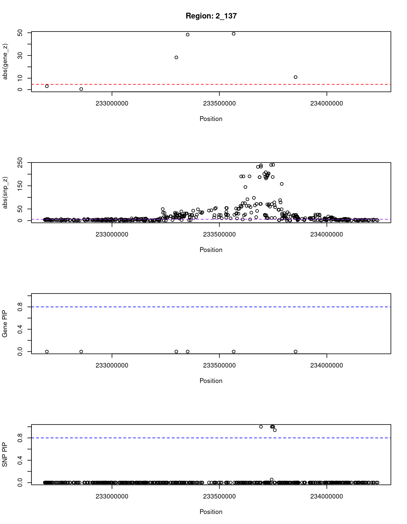
| Version | Author | Date |
|---|---|---|
| dfd2b5f | wesleycrouse | 2021-09-07 |
[1] "Region: 19_15"
      genename region_tag susie_pip   mu2     PVE     z
4199      LSM4      19_15     0.108  6.53 2.4e-06 -0.98
4197    PGPEP1      19_15     0.115  6.94 2.7e-06 -0.87
8907    LRRC25      19_15     0.144  9.41 4.6e-06  1.52
4196     SSBP4      19_15     0.131  7.94 3.5e-06 -1.04
2112    ISYNA1      19_15     0.104  6.15 2.2e-06  0.86
2113       ELL      19_15     0.089  4.71 1.4e-06  0.26
2123      KXD1      19_15     0.122  7.20 3.0e-06  0.66
11192    UBA52      19_15     0.126  7.83 3.4e-06 -1.07
7904    KLHL26      19_15     0.088  4.76 1.4e-06 -0.58
52        UPF1      19_15     0.177 10.21 6.2e-06 -1.14
2115      COPE      19_15     0.087  4.54 1.4e-06 -0.03
2116     DDX49      19_15     0.084  4.40 1.3e-06 -0.43
2118     ARMC6      19_15     0.110  6.74 2.5e-06  0.81
599      SUGP2      19_15     0.230 13.60 1.1e-05  1.98
596   TMEM161A      19_15     0.087  4.49 1.3e-06 -0.06
11075    MEF2B      19_15     0.215 17.06 1.3e-05 -3.15
11817   BORCS8      19_15     0.119 14.57 5.9e-06 -3.14
595     RFXANK      19_15     0.315 16.63 1.8e-05 -2.43
4137      MAU2      19_15     0.147 74.30 3.7e-05 -9.61
7905   GATAD2A      19_15     0.084 18.88 5.4e-06  4.59
9879   NDUFA13      19_15     0.087 18.25 5.4e-06  4.47
9152     TSSK6      19_15     0.101  6.17 2.1e-06 -0.86
11726   YJEFN3      19_15     0.114 17.91 6.9e-06  3.92
6840     CILP2      19_15     0.096  5.97 2.0e-06  0.95
2128      PBX4      19_15     0.085  4.85 1.4e-06  0.95
597      LPAR2      19_15     0.098  9.57 3.2e-06  2.41
1235      GMIP      19_15     0.144 11.81 5.8e-06  2.28
2131   ATP13A1      19_15     0.157 53.03 2.8e-05  8.15
9450    ZNF101      19_15     0.084  5.17 1.5e-06  1.10
2126     ZNF14      19_15     0.103  6.10 2.1e-06 -0.77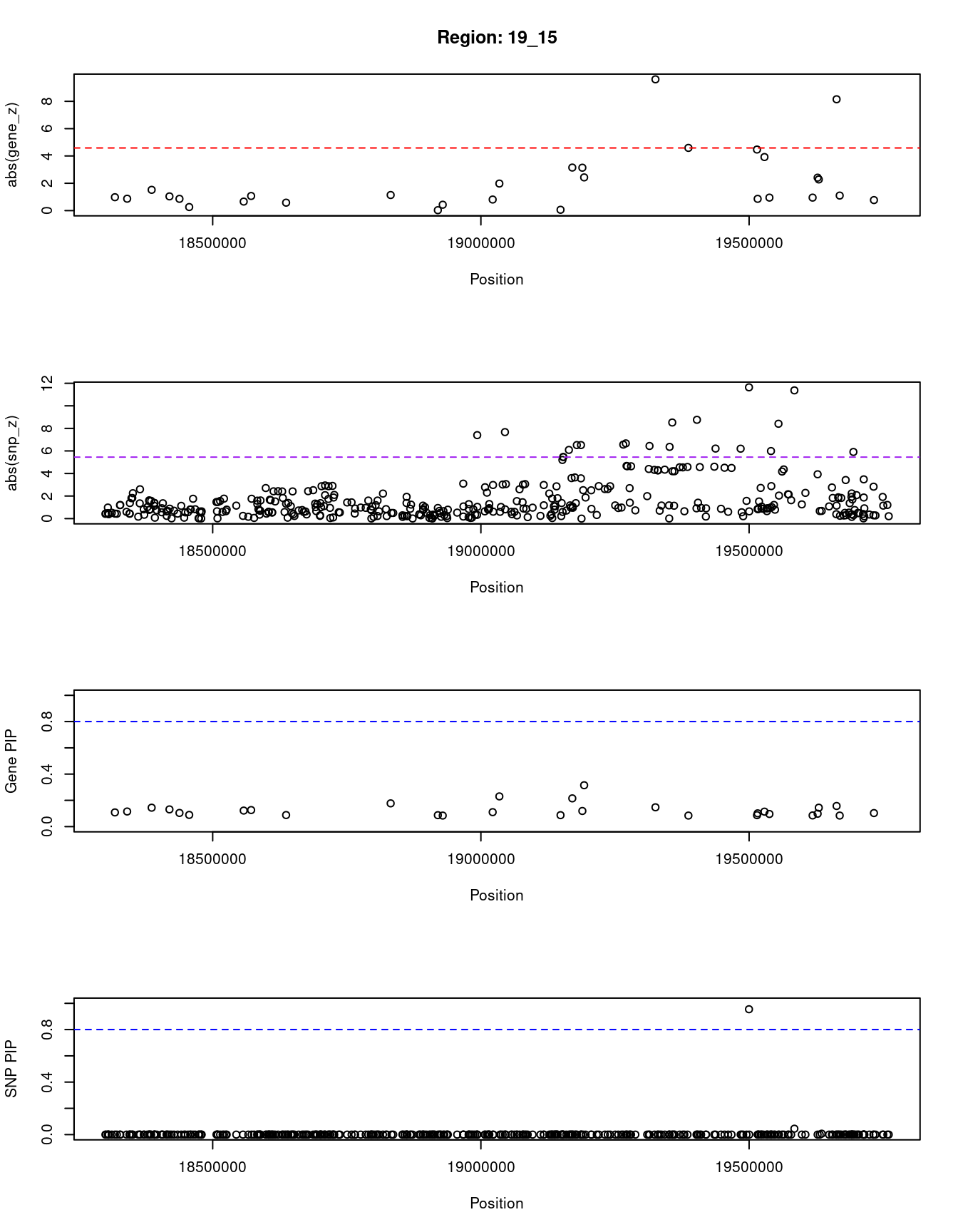
| Version | Author | Date |
|---|---|---|
| dfd2b5f | wesleycrouse | 2021-09-07 |
[1] "Region: 9_46"
          genename region_tag susie_pip   mu2     PVE     z
11350 RP11-305L7.1       9_46     0.116 21.70 8.6e-06 -4.57
7536         NFIL3       9_46     0.763 67.27 1.8e-04  9.30
5979           AUH       9_46     0.076 33.32 8.6e-06  6.47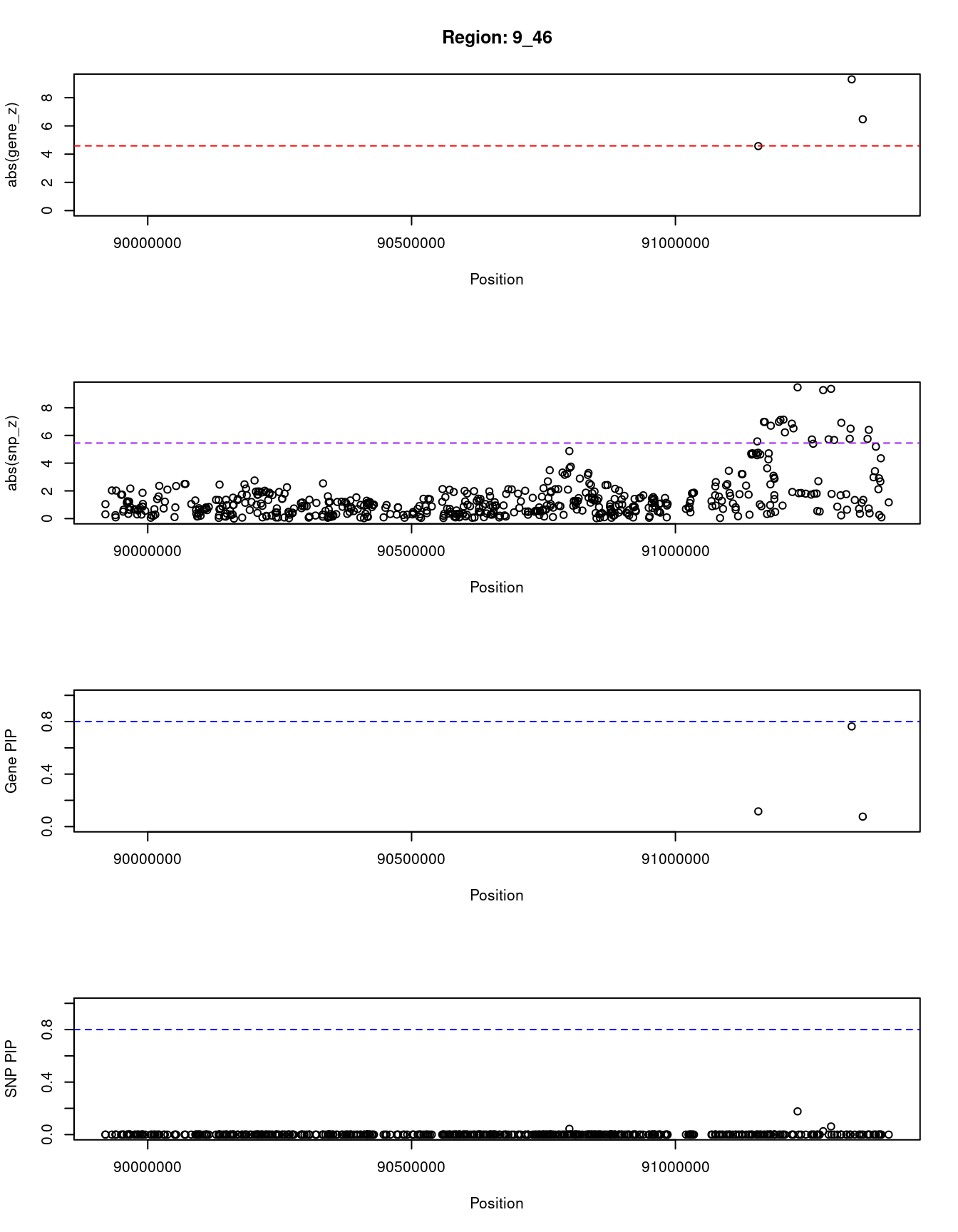
| Version | Author | Date |
|---|---|---|
| dfd2b5f | wesleycrouse | 2021-09-07 |
[1] "Region: 11_42"
           genename region_tag susie_pip   mu2     PVE     z
7739         RNF169      11_42     0.111  4.34 1.6e-06 -0.07
7737          XRRA1      11_42     0.115  4.62 1.8e-06 -0.23
3254          SPCS2      11_42     0.116  4.65 1.8e-06 -0.25
7029           NEU3      11_42     0.236 11.07 8.9e-06 -1.65
4988        SLCO2B1      11_42     0.169  8.06 4.6e-06  1.13
4987          ARRB1      11_42     0.267 13.02 1.2e-05  2.19
6070         KLHL35      11_42     0.173  8.48 5.0e-06  1.36
6706          GDPD5      11_42     0.327 14.79 1.7e-05 -2.39
6071       SERPINH1      11_42     0.110  4.89 1.8e-06 -0.98
562           DGAT2      11_42     0.962 45.37 1.5e-04 -7.48
10589         UVRAG      11_42     0.137  7.33 3.4e-06  1.62
1111          WNT11      11_42     0.115  4.85 1.9e-06 -0.69
4989         THAP12      11_42     0.118  5.02 2.0e-06 -0.70
12276 RP11-111M22.4      11_42     0.170  8.59 5.0e-06  1.45
11826 RP11-111M22.3      11_42     0.114  4.63 1.8e-06  0.47
11834  RP11-672A2.5      11_42     0.125  5.55 2.4e-06 -0.80
4996         LRRC32      11_42     0.115  4.73 1.8e-06 -0.59
11812  RP11-672A2.4      11_42     0.115  4.71 1.8e-06 -0.52
9528           TSKU      11_42     0.118  4.77 1.9e-06  0.25
949           ACER3      11_42     0.187  8.93 5.7e-06 -1.30
6072          CAPN5      11_42     0.124  5.38 2.3e-06  0.70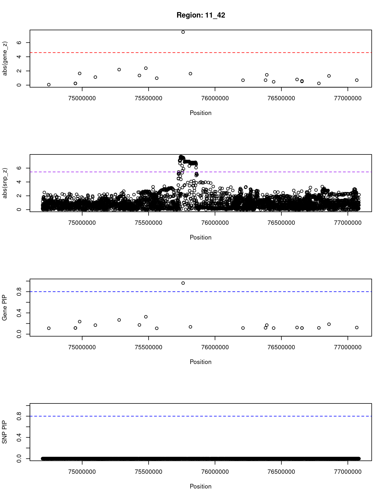
| Version | Author | Date |
|---|---|---|
| dfd2b5f | wesleycrouse | 2021-09-07 |
[1] "Region: 12_67"
          genename region_tag susie_pip   mu2     PVE     z
5228          TCHP      12_67     0.469 16.44 2.6e-05  3.46
5227          GIT2      12_67     0.519 16.42 2.9e-05  3.34
907       ANKRD13A      12_67     0.088  5.69 1.7e-06  0.55
8801      C12orf76      12_67     0.087  6.34 1.9e-06  1.85
3595         IFT81      12_67     0.085  7.03 2.0e-06  2.39
10285       ANAPC7      12_67     0.120  9.40 3.8e-06  2.33
2602         ARPC3      12_67     0.099  7.13 2.4e-06  1.32
10873      FAM216A      12_67     0.078  5.82 1.6e-06  1.89
2603          GPN3      12_67     0.086  7.41 2.2e-06  1.79
2604         VPS29      12_67     0.091  7.10 2.2e-06 -1.72
6173         RAD9B      12_67     0.091  7.10 2.2e-06 -1.72
10872        TCTN1      12_67     0.092  5.50 1.7e-06  0.27
3597         HVCN1      12_67     0.080  5.35 1.5e-06  1.79
9912        PPP1CC      12_67     0.148 11.84 6.0e-06 -2.65
10579      FAM109A      12_67     0.084 20.96 6.0e-06 -5.33
11891  RP3-473L9.4      12_67     0.089 24.35 7.4e-06 -5.72
2607         SH2B3      12_67     0.077 29.85 7.8e-06  6.80
10869        ATXN2      12_67     0.077  5.13 1.3e-06  0.63
2611         ALDH2      12_67     0.187 35.19 2.2e-05 -6.42
1210      MAPKAPK5      12_67     0.218 29.58 2.2e-05  6.30
11433 MAPKAPK5-AS1      12_67     0.151 36.20 1.9e-05 -7.24
1227         ERP29      12_67     0.204 28.77 2.0e-05  6.25
10574      TMEM116      12_67     0.204 28.77 2.0e-05 -6.25
2613         NAA25      12_67     0.175 26.73 1.6e-05 -6.12
8655        HECTD4      12_67     0.088  5.76 1.7e-06  1.03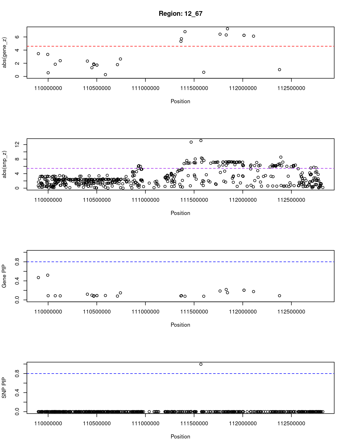
| Version | Author | Date |
|---|---|---|
| dfd2b5f | wesleycrouse | 2021-09-07 |
SNPs with highest PIPs
#snps with PIP>0.8 or 20 highest PIPs
head(ctwas_snp_res[order(-ctwas_snp_res$susie_pip),report_cols_snps],
max(sum(ctwas_snp_res$susie_pip>0.8), 20))
id region_tag susie_pip mu2 PVE z
131370 rs2070959 2_137 1.000 54893.97 0.19000 238.14
131398 rs76063448 2_137 1.000 8092.87 0.02800 70.66
131399 rs11888459 2_137 1.000 58654.69 0.20000 187.72
131400 rs2885296 2_137 1.000 77641.33 0.27000 240.61
320877 rs72834643 6_20 1.000 128.00 0.00044 9.73
320898 rs115740542 6_20 1.000 196.74 0.00067 12.66
372718 rs542176135 7_17 1.000 177.59 0.00061 -8.38
592225 rs11045819 12_16 1.000 5762.52 0.02000 -14.34
592242 rs4363657 12_16 1.000 1630.62 0.00560 43.78
782269 rs59616136 19_14 1.000 52.64 0.00018 7.00
893553 rs200216446 3_104 1.000 11592.56 0.04000 3.98
979421 rs662138 6_103 1.000 131.86 0.00045 -7.82
995224 rs17476364 10_46 1.000 291.55 0.00100 17.16
322068 rs3130253 6_23 0.999 48.88 0.00017 -6.63
372740 rs4721597 7_17 0.999 111.20 0.00038 1.94
498719 rs115478735 9_70 0.999 69.96 0.00024 -8.02
543879 rs76153913 11_2 0.998 53.33 0.00018 6.70
531451 rs111286300 10_64 0.997 42.64 0.00015 6.73
619055 rs653178 12_67 0.996 164.61 0.00056 -13.12
131050 rs4973550 2_136 0.994 45.50 0.00015 6.18
131061 rs6731991 2_136 0.989 40.55 0.00014 -5.75
591940 rs7962574 12_15 0.983 58.45 0.00020 -8.40
35871 rs2779116 1_79 0.982 73.12 0.00025 -8.25
696238 rs340029 15_27 0.978 48.46 0.00016 -6.60
1125927 rs429358 19_31 0.956 47.26 0.00015 -8.01
783054 rs3794991 19_15 0.955 135.01 0.00044 11.64
131403 rs12052787 2_137 0.939 2606.88 0.00840 -11.25
591980 rs10770693 12_15 0.934 66.87 0.00021 8.86
484922 rs9410381 9_45 0.923 78.90 0.00025 8.62
893552 rs12492030 3_104 0.915 11508.95 0.03600 2.70
428128 rs12549737 8_24 0.908 37.04 0.00011 5.15
1125928 rs7412 19_31 0.901 206.58 0.00064 15.02
320716 rs75080831 6_19 0.861 67.97 0.00020 7.96
321447 rs156737 6_21 0.842 42.94 0.00012 -6.37
546901 rs4910498 11_8 0.834 51.96 0.00015 6.71
592126 rs12366506 12_16 0.805 4963.57 0.01400 23.44
831840 rs6000553 22_14 0.802 46.70 0.00013 6.47SNPs with largest effect sizes
#plot PIP vs effect size
plot(ctwas_snp_res$susie_pip, ctwas_snp_res$mu2, xlab="PIP", ylab="mu^2", main="SNP PIPs vs Effect Size")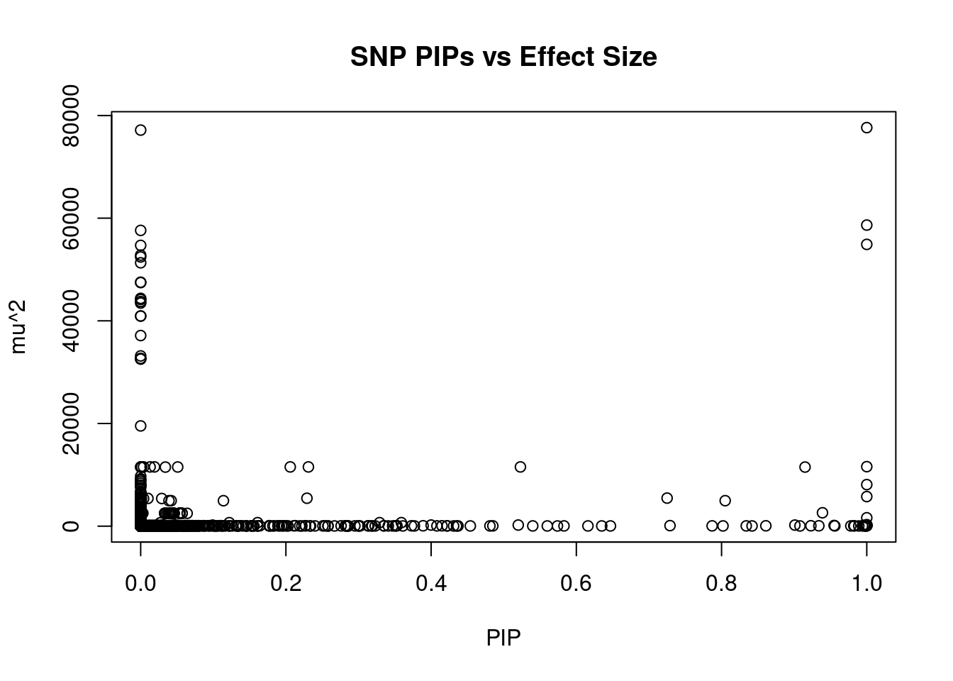
| Version | Author | Date |
|---|---|---|
| dfd2b5f | wesleycrouse | 2021-09-07 |
#SNPs with 50 largest effect sizes
head(ctwas_snp_res[order(-ctwas_snp_res$mu2),report_cols_snps],50)
id region_tag susie_pip mu2 PVE z
131400 rs2885296 2_137 1.000 77641.33 2.7e-01 240.61
131396 rs17862875 2_137 0.000 77157.58 0.0e+00 239.53
131399 rs11888459 2_137 1.000 58654.69 2.0e-01 187.72
131382 rs13401281 2_137 0.000 57619.63 6.6e-17 186.34
131370 rs2070959 2_137 1.000 54893.97 1.9e-01 238.14
131379 rs1875263 2_137 0.000 54699.90 4.0e-15 181.67
131369 rs1105880 2_137 0.000 52801.38 0.0e+00 232.16
131364 rs77070100 2_137 0.000 52439.87 0.0e+00 231.38
131378 rs6749496 2_137 0.000 51307.72 0.0e+00 208.13
131389 rs57258852 2_137 0.000 47524.59 0.0e+00 198.41
131371 rs7583278 2_137 0.000 47449.33 0.0e+00 200.99
131387 rs4663332 2_137 0.000 44379.07 0.0e+00 194.41
131388 rs200973045 2_137 0.000 44157.79 0.0e+00 194.10
131393 rs3821242 2_137 0.000 43759.17 0.0e+00 203.17
131391 rs2008584 2_137 0.000 43467.63 0.0e+00 202.59
131365 rs6753320 2_137 0.000 40935.47 0.0e+00 186.96
131366 rs6736743 2_137 0.000 40935.47 0.0e+00 186.96
131377 rs2012734 2_137 0.000 37131.98 0.0e+00 187.89
131414 rs2361502 2_137 0.000 33164.71 0.0e+00 157.91
131355 rs2741034 2_137 0.000 32680.28 0.0e+00 190.53
131347 rs2602363 2_137 0.000 32629.21 0.0e+00 190.40
131342 rs2741013 2_137 0.000 32542.16 0.0e+00 190.21
131351 rs6431558 2_137 0.000 19529.13 0.0e+00 -144.34
893553 rs200216446 3_104 1.000 11592.56 4.0e-02 3.98
893589 rs61791061 3_104 0.019 11540.28 7.6e-04 2.51
893588 rs74402546 3_104 0.013 11539.88 5.2e-04 2.50
893535 rs61793869 3_104 0.523 11537.17 2.1e-02 2.58
893544 rs61793896 3_104 0.206 11536.76 8.1e-03 2.56
893541 rs61793871 3_104 0.231 11536.73 9.1e-03 2.57
893596 rs12493271 3_104 0.004 11533.55 1.6e-04 2.49
893584 rs12495549 3_104 0.000 11532.76 3.1e-06 2.49
893629 rs12490982 3_104 0.001 11528.00 3.4e-05 2.56
893631 rs61791071 3_104 0.001 11527.18 3.8e-05 2.56
893623 rs61791069 3_104 0.051 11526.00 2.0e-03 2.64
893664 rs61791108 3_104 0.001 11515.81 4.7e-05 2.59
893552 rs12492030 3_104 0.915 11508.95 3.6e-02 2.70
893570 rs12490945 3_104 0.000 11505.49 1.6e-05 2.63
893635 rs61791073 3_104 0.034 11504.65 1.3e-03 2.67
131412 rs6723936 2_137 0.000 9721.35 0.0e+00 78.31
893533 rs200983760 3_104 0.000 9221.08 5.6e-17 2.42
131353 rs1823803 2_137 0.000 9005.94 0.0e+00 91.76
131401 rs143373661 2_137 0.000 8729.69 0.0e+00 78.24
131411 rs10202032 2_137 0.000 8385.70 0.0e+00 -88.03
131398 rs76063448 2_137 1.000 8092.87 2.8e-02 70.66
131394 rs45510999 2_137 0.000 8009.35 0.0e+00 70.21
131368 rs12476197 2_137 0.000 7953.56 0.0e+00 -71.92
131386 rs183532563 2_137 0.000 7941.29 0.0e+00 69.70
131362 rs4663871 2_137 0.000 7907.86 0.0e+00 -71.72
131367 rs765251456 2_137 0.000 7835.40 0.0e+00 -71.57
131359 rs1113193 2_137 0.000 7490.62 0.0e+00 -97.79SNPs with highest PVE
#SNPs with 50 highest pve
head(ctwas_snp_res[order(-ctwas_snp_res$PVE),report_cols_snps],50)
id region_tag susie_pip mu2 PVE z
131400 rs2885296 2_137 1.000 77641.33 0.27000 240.61
131399 rs11888459 2_137 1.000 58654.69 0.20000 187.72
131370 rs2070959 2_137 1.000 54893.97 0.19000 238.14
893553 rs200216446 3_104 1.000 11592.56 0.04000 3.98
893552 rs12492030 3_104 0.915 11508.95 0.03600 2.70
131398 rs76063448 2_137 1.000 8092.87 0.02800 70.66
893535 rs61793869 3_104 0.523 11537.17 0.02100 2.58
592225 rs11045819 12_16 1.000 5762.52 0.02000 -14.34
592126 rs12366506 12_16 0.805 4963.57 0.01400 23.44
592212 rs12371691 12_16 0.725 5463.31 0.01400 7.75
893541 rs61793871 3_104 0.231 11536.73 0.00910 2.57
131403 rs12052787 2_137 0.939 2606.88 0.00840 -11.25
893544 rs61793896 3_104 0.206 11536.76 0.00810 2.56
592242 rs4363657 12_16 1.000 1630.62 0.00560 43.78
592206 rs17328763 12_16 0.229 5440.15 0.00430 7.87
893623 rs61791069 3_104 0.051 11526.00 0.00200 2.64
592132 rs11045612 12_16 0.114 4957.26 0.00190 23.44
893635 rs61791073 3_104 0.034 11504.65 0.00130 2.67
995224 rs17476364 10_46 1.000 291.55 0.00100 17.16
592036 rs3060461 12_16 0.359 685.69 0.00084 -21.86
592040 rs35290079 12_16 0.329 681.86 0.00077 -21.76
893589 rs61791061 3_104 0.019 11540.28 0.00076 2.51
592143 rs73062442 12_16 0.042 4962.31 0.00071 23.39
320898 rs115740542 6_20 1.000 196.74 0.00067 12.66
592135 rs11513221 12_16 0.039 4962.78 0.00066 23.38
1125928 rs7412 19_31 0.901 206.58 0.00064 15.02
372718 rs542176135 7_17 1.000 177.59 0.00061 -8.38
619055 rs653178 12_67 0.996 164.61 0.00056 -13.12
893555 rs547661537 3_104 0.064 2495.75 0.00055 4.85
592186 rs11045737 12_16 0.029 5388.64 0.00053 9.34
893588 rs74402546 3_104 0.013 11539.88 0.00052 2.50
893550 rs9754613 3_104 0.057 2499.65 0.00049 4.85
893564 rs7646100 3_104 0.057 2508.36 0.00049 4.86
131397 rs3796088 2_137 0.054 2578.60 0.00048 -11.12
893616 rs61791066 3_104 0.054 2496.23 0.00046 4.86
893652 rs11711437 3_104 0.053 2490.79 0.00045 4.89
979421 rs662138 6_103 1.000 131.86 0.00045 -7.82
320877 rs72834643 6_20 1.000 128.00 0.00044 9.73
783054 rs3794991 19_15 0.955 135.01 0.00044 11.64
893558 rs6766904 3_104 0.046 2507.87 0.00040 4.84
893569 rs12496734 3_104 0.046 2506.79 0.00039 4.83
893617 rs16855617 3_104 0.046 2496.42 0.00039 4.85
176638 rs523118 3_84 0.520 215.35 0.00038 -14.52
372740 rs4721597 7_17 0.999 111.20 0.00038 1.94
592042 rs7965380 12_16 0.161 681.10 0.00038 -21.74
893548 rs137914315 3_104 0.044 2507.84 0.00038 4.83
893572 rs11720640 3_104 0.045 2506.77 0.00038 4.83
893592 rs16847990 3_104 0.043 2496.27 0.00037 4.84
893542 rs6780208 3_104 0.042 2508.01 0.00036 4.82
893571 rs16855595 3_104 0.042 2506.66 0.00036 4.82SNPs with largest z scores
#SNPs with 50 largest z scores
head(ctwas_snp_res[order(-abs(ctwas_snp_res$z)),report_cols_snps],50)
id region_tag susie_pip mu2 PVE z
131400 rs2885296 2_137 1 77641.33 2.7e-01 240.61
131396 rs17862875 2_137 0 77157.58 0.0e+00 239.53
131370 rs2070959 2_137 1 54893.97 1.9e-01 238.14
131369 rs1105880 2_137 0 52801.38 0.0e+00 232.16
131364 rs77070100 2_137 0 52439.87 0.0e+00 231.38
131378 rs6749496 2_137 0 51307.72 0.0e+00 208.13
131393 rs3821242 2_137 0 43759.17 0.0e+00 203.17
131391 rs2008584 2_137 0 43467.63 0.0e+00 202.59
131371 rs7583278 2_137 0 47449.33 0.0e+00 200.99
131389 rs57258852 2_137 0 47524.59 0.0e+00 198.41
131387 rs4663332 2_137 0 44379.07 0.0e+00 194.41
131388 rs200973045 2_137 0 44157.79 0.0e+00 194.10
131355 rs2741034 2_137 0 32680.28 0.0e+00 190.53
131347 rs2602363 2_137 0 32629.21 0.0e+00 190.40
131342 rs2741013 2_137 0 32542.16 0.0e+00 190.21
131377 rs2012734 2_137 0 37131.98 0.0e+00 187.89
131399 rs11888459 2_137 1 58654.69 2.0e-01 187.72
131365 rs6753320 2_137 0 40935.47 0.0e+00 186.96
131366 rs6736743 2_137 0 40935.47 0.0e+00 186.96
131382 rs13401281 2_137 0 57619.63 6.6e-17 186.34
131379 rs1875263 2_137 0 54699.90 4.0e-15 181.67
131414 rs2361502 2_137 0 33164.71 0.0e+00 157.91
131351 rs6431558 2_137 0 19529.13 0.0e+00 -144.34
131359 rs1113193 2_137 0 7490.62 0.0e+00 -97.79
131353 rs1823803 2_137 0 9005.94 0.0e+00 91.76
131411 rs10202032 2_137 0 8385.70 0.0e+00 -88.03
131412 rs6723936 2_137 0 9721.35 0.0e+00 78.31
131401 rs143373661 2_137 0 8729.69 0.0e+00 78.24
131349 rs13027376 2_137 0 6689.85 0.0e+00 -74.88
131346 rs4047192 2_137 0 6680.63 0.0e+00 -74.81
131368 rs12476197 2_137 0 7953.56 0.0e+00 -71.92
131362 rs4663871 2_137 0 7907.86 0.0e+00 -71.72
131367 rs765251456 2_137 0 7835.40 0.0e+00 -71.57
131398 rs76063448 2_137 1 8092.87 2.8e-02 70.66
131394 rs45510999 2_137 0 8009.35 0.0e+00 70.21
131386 rs183532563 2_137 0 7941.29 0.0e+00 69.70
131402 rs11568318 2_137 0 1456.69 0.0e+00 -65.81
131392 rs45507691 2_137 0 1447.76 0.0e+00 -65.58
131360 rs17863773 2_137 0 6272.97 0.0e+00 -65.44
131354 rs10929252 2_137 0 5364.72 0.0e+00 -63.60
131352 rs17863766 2_137 0 5247.57 0.0e+00 -63.58
131341 rs140719475 2_137 0 5353.33 0.0e+00 -63.55
131344 rs6713902 2_137 0 4574.18 0.0e+00 -60.77
131395 rs139257330 2_137 0 5353.51 0.0e+00 60.10
131343 rs7563478 2_137 0 1129.82 0.0e+00 -59.73
131357 rs2602372 2_137 0 4816.02 0.0e+00 58.13
131404 rs2003569 2_137 0 3754.14 4.7e-08 -57.58
131327 rs62192764 2_137 0 3156.88 0.0e+00 -54.32
131319 rs62192761 2_137 0 3141.73 0.0e+00 -54.28
131329 rs4047189 2_137 0 4177.45 0.0e+00 53.85Gene set enrichment for genes with PIP>0.8
#GO enrichment analysis
library(enrichR)
Welcome to enrichR
Checking connection ... Enrichr ... Connection is Live!
FlyEnrichr ... Connection is available!
WormEnrichr ... Connection is available!
YeastEnrichr ... Connection is available!
FishEnrichr ... Connection is available!dbs <- c("GO_Biological_Process_2021", "GO_Cellular_Component_2021", "GO_Molecular_Function_2021")
genes <- ctwas_gene_res$genename[ctwas_gene_res$susie_pip>0.8]
#number of genes for gene set enrichment
length(genes)[1] 49if (length(genes)>0){
GO_enrichment <- enrichr(genes, dbs)
for (db in dbs){
print(db)
df <- GO_enrichment[[db]]
df <- df[df$Adjusted.P.value<0.05,c("Term", "Overlap", "Adjusted.P.value", "Genes")]
print(df)
}
#DisGeNET enrichment
# devtools::install_bitbucket("ibi_group/disgenet2r")
library(disgenet2r)
disgenet_api_key <- get_disgenet_api_key(
email = "wesleycrouse@gmail.com",
password = "uchicago1" )
Sys.setenv(DISGENET_API_KEY= disgenet_api_key)
res_enrich <-disease_enrichment(entities=genes, vocabulary = "HGNC",
database = "CURATED" )
df <- res_enrich@qresult[1:10, c("Description", "FDR", "Ratio", "BgRatio")]
print(df)
#WebGestalt enrichment
library(WebGestaltR)
background <- ctwas_gene_res$genename
#listGeneSet()
databases <- c("pathway_KEGG", "disease_GLAD4U", "disease_OMIM")
enrichResult <- WebGestaltR(enrichMethod="ORA", organism="hsapiens",
interestGene=genes, referenceGene=background,
enrichDatabase=databases, interestGeneType="genesymbol",
referenceGeneType="genesymbol", isOutput=F)
print(enrichResult[,c("description", "size", "overlap", "FDR", "database", "userId")])
}Uploading data to Enrichr... Done.
Querying GO_Biological_Process_2021... Done.
Querying GO_Cellular_Component_2021... Done.
Querying GO_Molecular_Function_2021... Done.
Parsing results... Done.
[1] "GO_Biological_Process_2021"
[1] Term Overlap Adjusted.P.value Genes
<0 rows> (or 0-length row.names)
[1] "GO_Cellular_Component_2021"
[1] Term Overlap Adjusted.P.value Genes
<0 rows> (or 0-length row.names)
[1] "GO_Molecular_Function_2021"
[1] Term Overlap Adjusted.P.value Genes
<0 rows> (or 0-length row.names)RP11-9M16.2 gene(s) from the input list not found in DisGeNET CURATEDHKDC1 gene(s) from the input list not found in DisGeNET CURATEDRNFT1 gene(s) from the input list not found in DisGeNET CURATEDICA1L gene(s) from the input list not found in DisGeNET CURATEDTXNDC11 gene(s) from the input list not found in DisGeNET CURATEDUNK gene(s) from the input list not found in DisGeNET CURATEDTBL2 gene(s) from the input list not found in DisGeNET CURATEDSMIM19 gene(s) from the input list not found in DisGeNET CURATEDRP11-88E10.5 gene(s) from the input list not found in DisGeNET CURATEDRASIP1 gene(s) from the input list not found in DisGeNET CURATEDZCCHC24 gene(s) from the input list not found in DisGeNET CURATEDCEP44 gene(s) from the input list not found in DisGeNET CURATEDSIK2 gene(s) from the input list not found in DisGeNET CURATEDRRBP1 gene(s) from the input list not found in DisGeNET CURATEDDRC3 gene(s) from the input list not found in DisGeNET CURATEDRP11-334C17.6 gene(s) from the input list not found in DisGeNET CURATEDCSNK1G3 gene(s) from the input list not found in DisGeNET CURATEDSMG6 gene(s) from the input list not found in DisGeNET CURATEDARHGAP25 gene(s) from the input list not found in DisGeNET CURATEDSCAF11 gene(s) from the input list not found in DisGeNET CURATEDCNIH4 gene(s) from the input list not found in DisGeNET CURATED Description
95 Chromosome Breaks
100 Chromosome Breakage
92 Vesicular Stomatitis
140 Preeclampsia Eclampsia 4
162 SHASHI-PENA SYNDROME
163 IMMUNODEFICIENCY-CENTROMERIC INSTABILITY-FACIAL ANOMALIES SYNDROME 1
165 DEVELOPMENTAL DELAY, INTELLECTUAL DISABILITY, OBESITY, AND DYSMORPHIC FEATURES
51 Acute Myeloid Leukemia, M1
115 Nephroblastomatosis, fetal ascites, macrosomia and Wilms tumor
139 FACIOSCAPULOHUMERAL MUSCULAR DYSTROPHY 1B
FDR Ratio BgRatio
95 0.06010904 2/28 14/9703
100 0.06010904 2/28 14/9703
92 0.06926407 1/28 1/9703
140 0.06926407 1/28 1/9703
162 0.06926407 1/28 1/9703
163 0.06926407 1/28 1/9703
165 0.06926407 1/28 1/9703
51 0.08069563 3/28 125/9703
115 0.08069563 1/28 2/9703
139 0.08069563 1/28 2/9703******************************************
* *
* Welcome to WebGestaltR ! *
* *
******************************************Loading the functional categories...
Loading the ID list...
Loading the reference list...
Performing the enrichment analysis...Warning in oraEnrichment(interestGeneList, referenceGeneList, geneSet,
minNum = minNum, : No significant gene set is identified based on FDR 0.05!NULL
sessionInfo()R version 3.6.1 (2019-07-05)
Platform: x86_64-pc-linux-gnu (64-bit)
Running under: Scientific Linux 7.4 (Nitrogen)
Matrix products: default
BLAS/LAPACK: /software/openblas-0.2.19-el7-x86_64/lib/libopenblas_haswellp-r0.2.19.so
locale:
[1] LC_CTYPE=en_US.UTF-8 LC_NUMERIC=C
[3] LC_TIME=en_US.UTF-8 LC_COLLATE=en_US.UTF-8
[5] LC_MONETARY=en_US.UTF-8 LC_MESSAGES=en_US.UTF-8
[7] LC_PAPER=en_US.UTF-8 LC_NAME=C
[9] LC_ADDRESS=C LC_TELEPHONE=C
[11] LC_MEASUREMENT=en_US.UTF-8 LC_IDENTIFICATION=C
attached base packages:
[1] stats graphics grDevices utils datasets methods base
other attached packages:
[1] WebGestaltR_0.4.4 disgenet2r_0.99.2 enrichR_3.0 cowplot_1.0.0
[5] ggplot2_3.3.3
loaded via a namespace (and not attached):
[1] bitops_1.0-6 matrixStats_0.57.0
[3] fs_1.3.1 bit64_4.0.5
[5] doParallel_1.0.16 progress_1.2.2
[7] httr_1.4.1 rprojroot_2.0.2
[9] GenomeInfoDb_1.20.0 doRNG_1.8.2
[11] tools_3.6.1 utf8_1.2.1
[13] R6_2.5.0 DBI_1.1.1
[15] BiocGenerics_0.30.0 colorspace_1.4-1
[17] withr_2.4.1 tidyselect_1.1.0
[19] prettyunits_1.0.2 bit_4.0.4
[21] curl_3.3 compiler_3.6.1
[23] git2r_0.26.1 Biobase_2.44.0
[25] DelayedArray_0.10.0 rtracklayer_1.44.0
[27] labeling_0.3 scales_1.1.0
[29] readr_1.4.0 apcluster_1.4.8
[31] stringr_1.4.0 digest_0.6.20
[33] Rsamtools_2.0.0 svglite_1.2.2
[35] rmarkdown_1.13 XVector_0.24.0
[37] pkgconfig_2.0.3 htmltools_0.3.6
[39] fastmap_1.1.0 BSgenome_1.52.0
[41] rlang_0.4.11 RSQLite_2.2.7
[43] generics_0.0.2 farver_2.1.0
[45] jsonlite_1.6 BiocParallel_1.18.0
[47] dplyr_1.0.7 VariantAnnotation_1.30.1
[49] RCurl_1.98-1.1 magrittr_2.0.1
[51] GenomeInfoDbData_1.2.1 Matrix_1.2-18
[53] Rcpp_1.0.6 munsell_0.5.0
[55] S4Vectors_0.22.1 fansi_0.5.0
[57] gdtools_0.1.9 lifecycle_1.0.0
[59] stringi_1.4.3 whisker_0.3-2
[61] yaml_2.2.0 SummarizedExperiment_1.14.1
[63] zlibbioc_1.30.0 plyr_1.8.4
[65] grid_3.6.1 blob_1.2.1
[67] parallel_3.6.1 promises_1.0.1
[69] crayon_1.4.1 lattice_0.20-38
[71] Biostrings_2.52.0 GenomicFeatures_1.36.3
[73] hms_1.1.0 knitr_1.23
[75] pillar_1.6.1 igraph_1.2.4.1
[77] GenomicRanges_1.36.0 rjson_0.2.20
[79] rngtools_1.5 codetools_0.2-16
[81] reshape2_1.4.3 biomaRt_2.40.1
[83] stats4_3.6.1 XML_3.98-1.20
[85] glue_1.4.2 evaluate_0.14
[87] data.table_1.14.0 foreach_1.5.1
[89] vctrs_0.3.8 httpuv_1.5.1
[91] gtable_0.3.0 purrr_0.3.4
[93] assertthat_0.2.1 cachem_1.0.5
[95] xfun_0.8 later_0.8.0
[97] tibble_3.1.2 iterators_1.0.13
[99] GenomicAlignments_1.20.1 AnnotationDbi_1.46.0
[101] memoise_2.0.0 IRanges_2.18.1
[103] workflowr_1.6.2 ellipsis_0.3.2