Direct bilirubin (quantile) - Liver [standard analysis]
wesleycrouse
2021-08-18
Last updated: 2023-07-27
Checks: 7 0
Knit directory: ctwas_applied/
This reproducible R Markdown analysis was created with workflowr (version 1.7.0). The Checks tab describes the reproducibility checks that were applied when the results were created. The Past versions tab lists the development history.
Great! Since the R Markdown file has been committed to the Git repository, you know the exact version of the code that produced these results.
Great job! The global environment was empty. Objects defined in the global environment can affect the analysis in your R Markdown file in unknown ways. For reproduciblity it’s best to always run the code in an empty environment.
The command set.seed(20210726) was run prior to running
the code in the R Markdown file. Setting a seed ensures that any results
that rely on randomness, e.g. subsampling or permutations, are
reproducible.
Great job! Recording the operating system, R version, and package versions is critical for reproducibility.
Nice! There were no cached chunks for this analysis, so you can be confident that you successfully produced the results during this run.
Great job! Using relative paths to the files within your workflowr project makes it easier to run your code on other machines.
Great! You are using Git for version control. Tracking code development and connecting the code version to the results is critical for reproducibility.
The results in this page were generated with repository version 05b0117. See the Past versions tab to see a history of the changes made to the R Markdown and HTML files.
Note that you need to be careful to ensure that all relevant files for
the analysis have been committed to Git prior to generating the results
(you can use wflow_publish or
wflow_git_commit). workflowr only checks the R Markdown
file, but you know if there are other scripts or data files that it
depends on. Below is the status of the Git repository when the results
were generated:
Untracked files:
    Untracked:  gwas.RData
    Untracked:  ld_R_info.RData
    Untracked:  z_snp_pos_ebi-a-GCST004131.RData
    Untracked:  z_snp_pos_ebi-a-GCST004132.RData
    Untracked:  z_snp_pos_ebi-a-GCST004133.RData
    Untracked:  z_snp_pos_scz-2018.RData
    Untracked:  z_snp_pos_ukb-a-360.RData
    Untracked:  z_snp_pos_ukb-d-30780_irnt.RData

Unstaged changes:
    Modified:   analysis/variance_prior_testing.Rmd
Note that any generated files, e.g. HTML, png, CSS, etc., are not included in this status report because it is ok for generated content to have uncommitted changes.
These are the previous versions of the repository in which changes were
made to the R Markdown
(analysis/ukb-d-30660_irnt_Liver_new.Rmd) and HTML
(docs/ukb-d-30660_irnt_Liver_new.html) files. If you’ve
configured a remote Git repository (see ?wflow_git_remote),
click on the hyperlinks in the table below to view the files as they
were in that past version.
| File | Version | Author | Date | Message |
|---|---|---|---|---|
| html | 05b0117 | wesleycrouse | 2023-07-27 | adding results for inv-gamma prior on variance |
| html | 57fd2c7 | wesleycrouse | 2021-09-13 | updating reports |
| html | 7e22565 | wesleycrouse | 2021-09-13 | updating reports |
| html | db3f58c | wesleycrouse | 2021-09-08 | adding enrichment to reports |
| html | cbf7408 | wesleycrouse | 2021-09-08 | adding enrichment to reports |
| html | a5fc17b | wesleycrouse | 2021-09-08 | updating reports |
| html | 4970e3e | wesleycrouse | 2021-09-08 | updating reports |
| html | 1b58868 | wesleycrouse | 2021-09-07 | regenerating reports |
| html | dfd2b5f | wesleycrouse | 2021-09-07 | regenerating reports |
| html | 28bdbcc | wesleycrouse | 2021-09-06 | fixing thin argument for fixed pi results |
| html | 47f58ac | wesleycrouse | 2021-09-06 | fixing thin argument for fixed pi results |
| Rmd | aa84813 | wesleycrouse | 2021-09-06 | updating additional analyses |
| Rmd | 209346f | wesleycrouse | 2021-09-06 | updating additional analyses |
| html | aa84813 | wesleycrouse | 2021-09-06 | updating additional analyses |
| html | 209346f | wesleycrouse | 2021-09-06 | updating additional analyses |
| html | 684574c | wesleycrouse | 2021-09-06 | switching from render to wflow_build |
| html | b14741c | wesleycrouse | 2021-09-06 | switching from render to wflow_build |
| html | a419d64 | wesleycrouse | 2021-09-06 | updated PVE calculation |
| html | 61b53b3 | wesleycrouse | 2021-09-06 | updated PVE calculation |
| html | b2c823e | wesleycrouse | 2021-09-01 | adding additional fixedsigma report |
| html | 837dd01 | wesleycrouse | 2021-09-01 | adding additional fixedsigma report |
| html | 1452ca8 | wesleycrouse | 2021-08-30 | fixing typo |
| html | 2739f4f | wesleycrouse | 2021-08-30 | fixing typo |
| html | bf1f4e8 | wesleycrouse | 2021-08-30 | fixing alignment on index |
| html | b1e6b7e | wesleycrouse | 2021-08-30 | fixing alignment on index |
| html | b0c3887 | wesleycrouse | 2021-08-30 | Adding detailed reports for 30660 |
| html | d7dfe76 | wesleycrouse | 2021-08-30 | Adding detailed reports for 30660 |
| Rmd | 09f9d28 | wesleycrouse | 2021-08-30 | Exploring fixed priors and trimming large z scores |
| Rmd | ea2e654 | wesleycrouse | 2021-08-30 | Exploring fixed priors and trimming large z scores |
Overview
These are the results of a ctwas analysis of the UK
Biobank trait Direct bilirubin (quantile) using
Liver gene weights.
The GWAS was conducted by the Neale Lab, and the biomarker traits we
analyzed are discussed here.
Summary statistics were obtained from IEU OpenGWAS using GWAS ID:
ukb-d-30660_irnt. Results were obtained from from IEU
rather than Neale Lab because they are in a standardard format (GWAS VCF). Note that 3 of
the 34 biomarker traits were not available from IEU and were excluded
from analysis.
The weights are mashr GTEx v8 models on Liver eQTL
obtained from PredictDB.
We performed a full harmonization of the variants, including recovering
strand ambiguous variants. This procedure is discussed in a separate
document. (TO-DO: add report that describes
harmonization)
LD matrices were computed from a 10% subset of Neale lab subjects. Subjects were matched using the plate and well information from genotyping. We included only biallelic variants with MAF>0.01 in the original Neale Lab GWAS. (TO-DO: add more details [number of subjects, variants, etc])
Weight QC
TO-DO: add enhanced QC reporting (total number of weights, why each variant was missing for all genes)
qclist_all <- list()

qc_files <- paste0(results_dir, "/", list.files(results_dir, pattern="exprqc.Rd"))

for (i in 1:length(qc_files)){
  load(qc_files[i])
  chr <- unlist(strsplit(rev(unlist(strsplit(qc_files[i], "_")))[1], "[.]"))[1]
  qclist_all[[chr]] <- cbind(do.call(rbind, lapply(qclist,unlist)), as.numeric(substring(chr,4)))
}

qclist_all <- data.frame(do.call(rbind, qclist_all))
colnames(qclist_all)[ncol(qclist_all)] <- "chr"

rm(qclist, wgtlist, z_gene_chr)

#number of imputed weights
nrow(qclist_all)
[1] 10901#number of imputed weights by chromosome
table(qclist_all$chr)
   1    2    3    4    5    6    7    8    9   10   11   12   13   14   15   16
1070  768  652  417  494  611  548  408  405  434  634  629  195  365  354  526
  17   18   19   20   21   22
 663  160  859  306  114  289
#proportion of imputed weights without missing variants
mean(qclist_all$nmiss==0)[1] 0.8365288Load ctwas results
#load ctwas results
ctwas_res <- data.table::fread(paste0(results_dir, "/", analysis_id, "_ctwas.susieIrss.txt"))

#make unique identifier for regions
ctwas_res$region_tag <- paste(ctwas_res$region_tag1, ctwas_res$region_tag2, sep="_")

#compute PVE for each gene/SNP
ctwas_res$PVE = ctwas_res$susie_pip*ctwas_res$mu/sample_size #check PVE calculation

#separate gene and SNP results
ctwas_gene_res <- ctwas_res[ctwas_res$type == "gene", ]
ctwas_gene_res <- data.frame(ctwas_gene_res)
ctwas_snp_res <- ctwas_res[ctwas_res$type == "SNP", ]
ctwas_snp_res <- data.frame(ctwas_snp_res)

#add gene information to results
sqlite <- RSQLite::dbDriver("SQLite")
db = RSQLite::dbConnect(sqlite, paste0("/project2/compbio/predictdb/mashr_models/mashr_", weight, ".db"))
query <- function(...) RSQLite::dbGetQuery(db, ...)
gene_info <- query("select gene, genename from extra")
gene_info <- query("select gene, genename, gene_type from extra")
RSQLite::dbDisconnect(db)

ctwas_gene_res <- cbind(ctwas_gene_res, gene_info[sapply(ctwas_gene_res$id, match, gene_info$gene), c("genename", "gene_type")])

#add z score to results
load(paste0(results_dir, "/", analysis_id, "_expr_z_gene.Rd"))
ctwas_gene_res$z <- z_gene[ctwas_gene_res$id,]$z

#load(paste0(results_dir, "/", analysis_id, "_expr_z_snp.Rd")) #for new version, stored after harmonization
z_snp <- readRDS(paste0(results_dir, "/", trait_id, ".RDS")) #for old version, unharmonized

z_snp <- z_snp[z_snp$id %in% ctwas_snp_res$id,] #subset snps to those included in analysis, note some are duplicated, need to match which allele was used
ctwas_snp_res$z <- z_snp$z[match(ctwas_snp_res$id, z_snp$id)] #for duplicated snps, this arbitrarily uses the first allele
ctwas_snp_res$z_flag <- as.numeric(ctwas_snp_res$id %in% z_snp$id[duplicated(z_snp$id)]) #mark the unclear z scores, flag=1

#formatting and rounding for tables
ctwas_gene_res$z <- round(ctwas_gene_res$z,2)
ctwas_snp_res$z <- round(ctwas_snp_res$z,2)
ctwas_gene_res$susie_pip <- round(ctwas_gene_res$susie_pip,3)
ctwas_snp_res$susie_pip <- round(ctwas_snp_res$susie_pip,3)
ctwas_gene_res$mu2 <- round(ctwas_gene_res$mu2,2)
ctwas_snp_res$mu2 <- round(ctwas_snp_res$mu2,2)
ctwas_gene_res$PVE <- signif(ctwas_gene_res$PVE, 2)
ctwas_snp_res$PVE <- signif(ctwas_snp_res$PVE, 2)

#merge gene and snp results with added information
ctwas_gene_res$z_flag=NA
ctwas_snp_res$genename=NA
ctwas_snp_res$gene_type=NA

ctwas_res <- rbind(ctwas_gene_res,
                   ctwas_snp_res[,colnames(ctwas_gene_res)])

#store columns to report
report_cols <- colnames(ctwas_gene_res)[!(colnames(ctwas_gene_res) %in% c("type", "region_tag1", "region_tag2", "cs_index", "gene_type", "z_flag", "id", "chrom", "pos"))]
first_cols <- c("genename", "region_tag")
report_cols <- c(first_cols, report_cols[!(report_cols %in% first_cols)])

report_cols_snps <- c("id", report_cols[-1])

#get number of SNPs from s1 results; adjust for thin
ctwas_res_s1 <- data.table::fread(paste0(results_dir, "/", analysis_id, "_ctwas.s1.susieIrss.txt"))
n_snps <- sum(ctwas_res_s1$type=="SNP")/thin
rm(ctwas_res_s1)
Check convergence of parameters
library(ggplot2)
library(cowplot)

load(paste0(results_dir, "/", analysis_id, "_ctwas.s2.susieIrssres.Rd"))

df <- data.frame(niter = rep(1:ncol(group_prior_rec), 2),
                 value = c(group_prior_rec[1,], group_prior_rec[2,]),
                 group = rep(c("Gene", "SNP"), each = ncol(group_prior_rec)))
df$group <- as.factor(df$group)

df$value[df$group=="SNP"] <- df$value[df$group=="SNP"]*thin #adjust parameter to account for thin argument

p_pi <- ggplot(df, aes(x=niter, y=value, group=group)) +
  geom_line(aes(color=group)) +
  geom_point(aes(color=group)) +
  xlab("Iteration") + ylab(bquote(pi)) +
  ggtitle("Prior mean") +
  theme_cowplot()

df <- data.frame(niter = rep(1:ncol(group_prior_var_rec), 2),
                 value = c(group_prior_var_rec[1,], group_prior_var_rec[2,]),
                 group = rep(c("Gene", "SNP"), each = ncol(group_prior_var_rec)))
df$group <- as.factor(df$group)
p_sigma2 <- ggplot(df, aes(x=niter, y=value, group=group)) +
  geom_line(aes(color=group)) +
  geom_point(aes(color=group)) +
  xlab("Iteration") + ylab(bquote(sigma^2)) +
  ggtitle("Prior variance") +
  theme_cowplot()

plot_grid(p_pi, p_sigma2)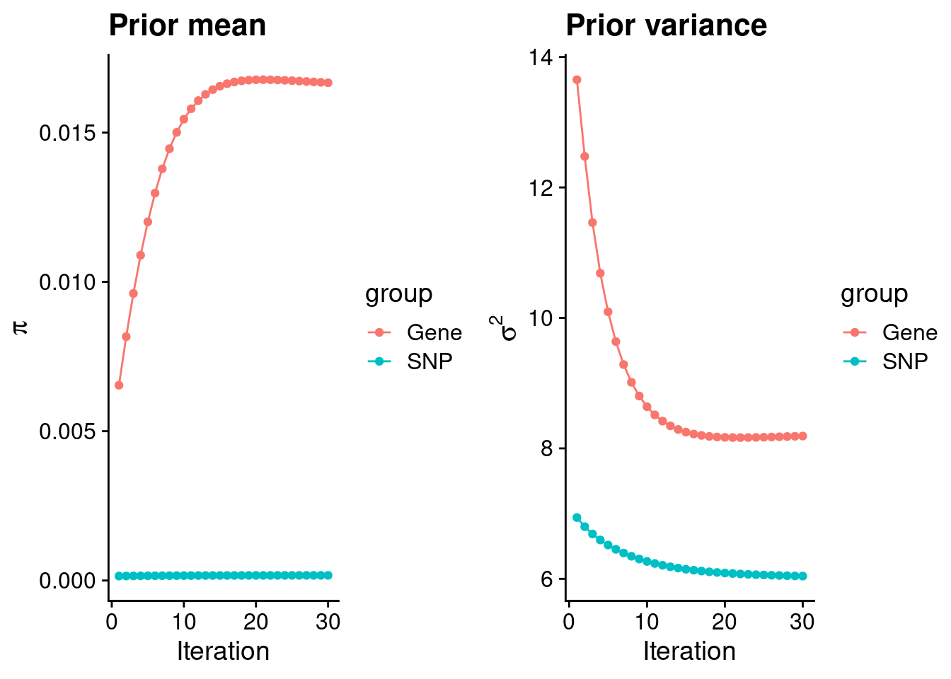
#estimated group prior
estimated_group_prior <- group_prior_rec[,ncol(group_prior_rec)]
names(estimated_group_prior) <- c("gene", "snp")
estimated_group_prior["snp"] <- estimated_group_prior["snp"]*thin #adjust parameter to account for thin argument
print(estimated_group_prior)
gene snp
0.0166666915 0.0001731877 #estimated group prior variance
estimated_group_prior_var <- group_prior_var_rec[,ncol(group_prior_var_rec)]
names(estimated_group_prior_var) <- c("gene", "snp")
print(estimated_group_prior_var) gene snp
8.188773 6.042154 #report sample size
print(sample_size)[1] 292933#report group size
group_size <- c(nrow(ctwas_gene_res), n_snps)
print(group_size)[1] 10876 8681670#estimated group PVE
estimated_group_pve <- estimated_group_prior_var*estimated_group_prior*group_size/sample_size #check PVE calculation
names(estimated_group_pve) <- c("gene", "snp")
print(estimated_group_pve) gene snp
0.005067213 0.031013005 #compare sum(PIP*mu2/sample_size) with above PVE calculation
c(sum(ctwas_gene_res$PVE),sum(ctwas_snp_res$PVE))[1] 0.02515714 0.26383586Genes with highest PIPs
#distribution of PIPs
hist(ctwas_gene_res$susie_pip, xlim=c(0,1), main="Distribution of Gene PIPs")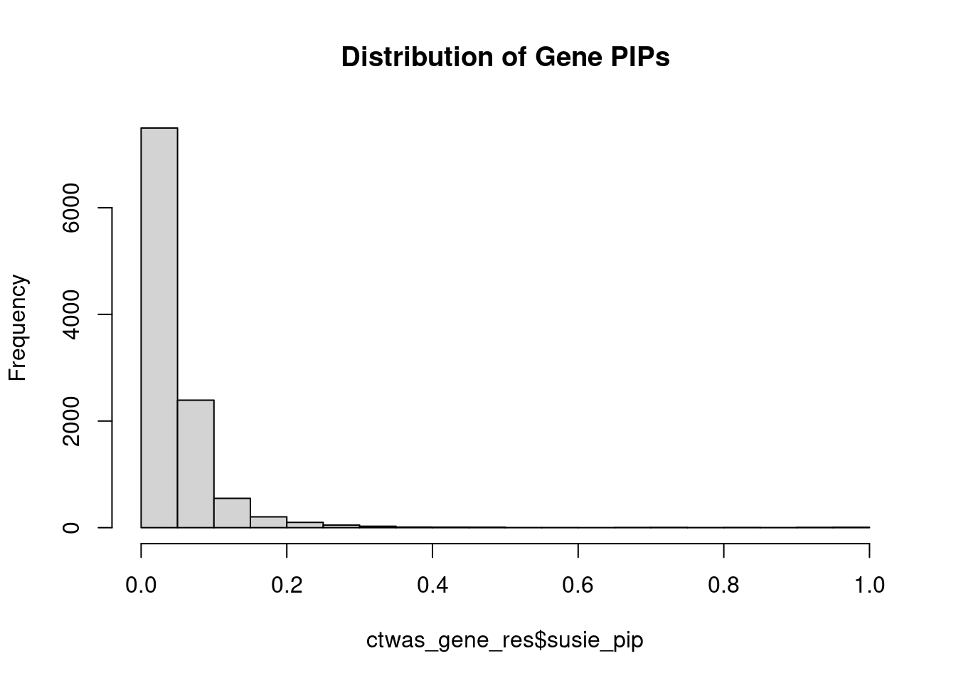
#genes with PIP>0.8 or 20 highest PIPs
head(ctwas_gene_res[order(-ctwas_gene_res$susie_pip),report_cols], max(sum(ctwas_gene_res$susie_pip>0.8), 20))
genename region_tag susie_pip mu2 PVE z
3212 CCND2 12_4 0.999 28.18 9.6e-05 5.34
12467 RP11-219B17.3 15_27 0.998 47.46 1.6e-04 7.18
1848 CD276 15_35 0.998 34.46 1.2e-04 6.13
7040 INHBB 2_70 0.995 23.55 8.0e-05 4.81
10667 HLA-G 6_24 0.975 38.44 1.3e-04 -6.69
11790 CYP2A6 19_28 0.960 22.30 7.3e-05 -4.73
1320 CWF19L1 10_64 0.958 30.61 1.0e-04 -7.09
12687 RP4-781K5.7 1_121 0.941 19.48 6.3e-05 -4.17
3562 ACVR1C 2_94 0.936 22.42 7.2e-05 4.62
10495 PRMT6 1_66 0.935 25.78 8.2e-05 5.14
5563 ABCG8 2_27 0.930 33.27 1.1e-04 5.88
2359 ABCC3 17_29 0.915 21.62 6.8e-05 4.38
2924 EFHD1 2_136 0.908 37.25 1.2e-04 6.05
7547 LIPC 15_26 0.892 19.62 6.0e-05 3.99
4269 ITGB4 17_42 0.854 21.77 6.3e-05 -4.91
1231 PABPC4 1_24 0.841 22.43 6.4e-05 4.52
6682 CYB5R1 1_102 0.840 19.39 5.6e-05 -3.95
10212 IL27 16_23 0.821 23.75 6.7e-05 -4.76
537 DGAT2 11_42 0.804 49.68 1.4e-04 -7.51
1120 CETP 16_31 0.758 22.52 5.8e-05 -4.03Genes with largest effect sizes
#plot PIP vs effect size
plot(ctwas_gene_res$susie_pip, ctwas_gene_res$mu2, xlab="PIP", ylab="mu^2", main="Gene PIPs vs Effect Size")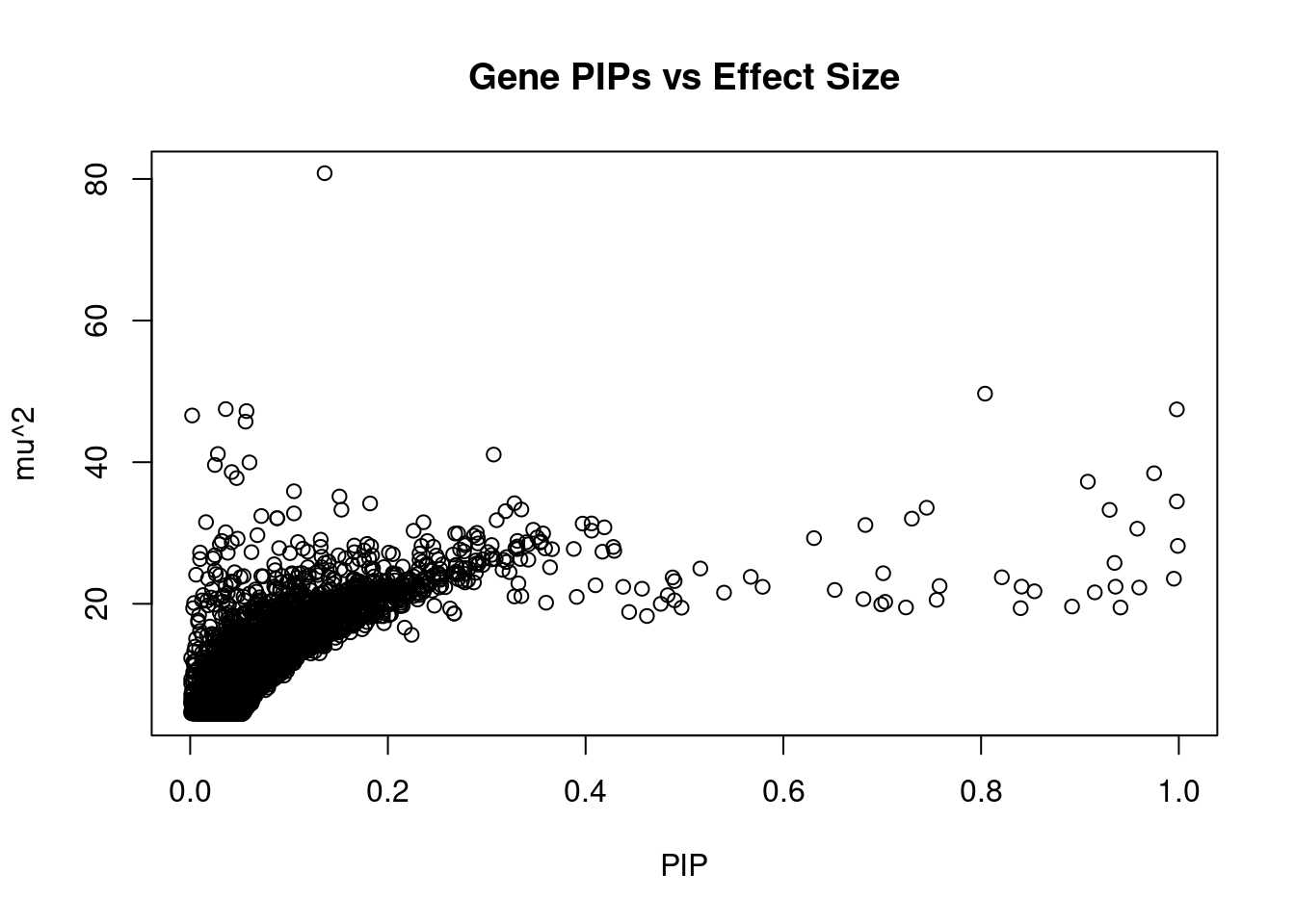
#genes with 20 largest effect sizes
head(ctwas_gene_res[order(-ctwas_gene_res$mu2),report_cols],20)
genename region_tag susie_pip mu2 PVE z
8651 MSL2 3_84 0.136 80.82 3.8e-05 10.28
537 DGAT2 11_42 0.804 49.68 1.4e-04 -7.51
3641 SLC17A1 6_20 0.036 47.50 5.8e-06 6.08
12467 RP11-219B17.3 15_27 0.998 47.46 1.6e-04 7.18
4962 EXOC6 10_59 0.057 47.22 9.2e-06 -6.37
823 TACR2 10_46 0.002 46.60 3.0e-07 3.90
2170 AHR 7_17 0.056 45.73 8.7e-06 -6.58
9850 HIST1H1C 6_20 0.028 41.16 3.9e-06 4.79
10214 ZNF165 6_22 0.307 41.08 4.3e-05 5.99
11290 MAPKAPK5-AS1 12_66 0.060 39.97 8.1e-06 -7.21
12379 U91328.22 6_20 0.025 39.61 3.4e-06 -4.74
5942 EIF4EBP2 10_46 0.042 38.61 5.5e-06 -3.06
10667 HLA-G 6_24 0.975 38.44 1.3e-04 -6.69
2541 ALDH2 12_66 0.047 37.76 6.0e-06 7.10
2924 EFHD1 2_136 0.908 37.25 1.2e-04 6.05
8505 HECTD4 12_66 0.105 35.90 1.3e-05 6.33
10734 NAP1L4 11_2 0.151 35.16 1.8e-05 3.47
1848 CD276 15_35 0.998 34.46 1.2e-04 6.13
1999 PRKD2 19_33 0.328 34.21 3.8e-05 -3.74
10425 AKR1C4 10_6 0.182 34.18 2.1e-05 6.16Genes with highest PVE
#genes with 20 highest pve
head(ctwas_gene_res[order(-ctwas_gene_res$PVE),report_cols],20)
genename region_tag susie_pip mu2 PVE z
12467 RP11-219B17.3 15_27 0.998 47.46 1.6e-04 7.18
537 DGAT2 11_42 0.804 49.68 1.4e-04 -7.51
10667 HLA-G 6_24 0.975 38.44 1.3e-04 -6.69
2924 EFHD1 2_136 0.908 37.25 1.2e-04 6.05
1848 CD276 15_35 0.998 34.46 1.2e-04 6.13
5563 ABCG8 2_27 0.930 33.27 1.1e-04 5.88
1320 CWF19L1 10_64 0.958 30.61 1.0e-04 -7.09
3212 CCND2 12_4 0.999 28.18 9.6e-05 5.34
10000 ZKSCAN3 6_22 0.745 33.57 8.5e-05 3.82
10495 PRMT6 1_66 0.935 25.78 8.2e-05 5.14
7040 INHBB 2_70 0.995 23.55 8.0e-05 4.81
2004 TGFB1 19_28 0.730 32.03 8.0e-05 5.64
11669 RP11-452H21.4 11_43 0.683 31.13 7.3e-05 5.78
11790 CYP2A6 19_28 0.960 22.30 7.3e-05 -4.73
3562 ACVR1C 2_94 0.936 22.42 7.2e-05 4.62
2359 ABCC3 17_29 0.915 21.62 6.8e-05 4.38
10212 IL27 16_23 0.821 23.75 6.7e-05 -4.76
1231 PABPC4 1_24 0.841 22.43 6.4e-05 4.52
12687 RP4-781K5.7 1_121 0.941 19.48 6.3e-05 -4.17
8142 CNTROB 17_7 0.631 29.28 6.3e-05 -5.71Genes with largest z scores
#genes with 20 largest z scores
head(ctwas_gene_res[order(-abs(ctwas_gene_res$z)),report_cols],20)
genename region_tag susie_pip mu2 PVE z
8651 MSL2 3_84 0.136 80.82 3.8e-05 10.28
537 DGAT2 11_42 0.804 49.68 1.4e-04 -7.51
11290 MAPKAPK5-AS1 12_66 0.060 39.97 8.1e-06 -7.21
12467 RP11-219B17.3 15_27 0.998 47.46 1.6e-04 7.18
2541 ALDH2 12_66 0.047 37.76 6.0e-06 7.10
1320 CWF19L1 10_64 0.958 30.61 1.0e-04 -7.09
2536 SH2B3 12_66 0.016 31.54 1.8e-06 6.80
10667 HLA-G 6_24 0.975 38.44 1.3e-04 -6.69
2170 AHR 7_17 0.056 45.73 8.7e-06 -6.58
4962 EXOC6 10_59 0.057 47.22 9.2e-06 -6.37
8505 HECTD4 12_66 0.105 35.90 1.3e-05 6.33
1191 ERP29 12_66 0.088 32.09 9.6e-06 6.25
10370 TMEM116 12_66 0.088 32.09 9.6e-06 -6.25
9829 ZKSCAN4 6_22 0.036 22.64 2.8e-06 -6.24
10425 AKR1C4 10_6 0.182 34.18 2.1e-05 6.16
1848 CD276 15_35 0.998 34.46 1.2e-04 6.13
2544 NAA25 12_66 0.068 29.70 6.9e-06 -6.12
3641 SLC17A1 6_20 0.036 47.50 5.8e-06 6.08
11216 CYP21A2 6_26 0.105 32.77 1.2e-05 -6.07
2924 EFHD1 2_136 0.908 37.25 1.2e-04 6.05Comparing z scores and PIPs
#set nominal signifiance threshold for z scores
alpha <- 0.05

#bonferroni adjusted threshold for z scores
sig_thresh <- qnorm(1-(alpha/nrow(ctwas_gene_res)/2), lower=T)

#Q-Q plot for z scores
obs_z <- ctwas_gene_res$z[order(ctwas_gene_res$z)]
exp_z <- qnorm((1:nrow(ctwas_gene_res))/nrow(ctwas_gene_res))

plot(exp_z, obs_z, xlab="Expected z", ylab="Observed z", main="Gene z score Q-Q plot")
abline(a=0,b=1)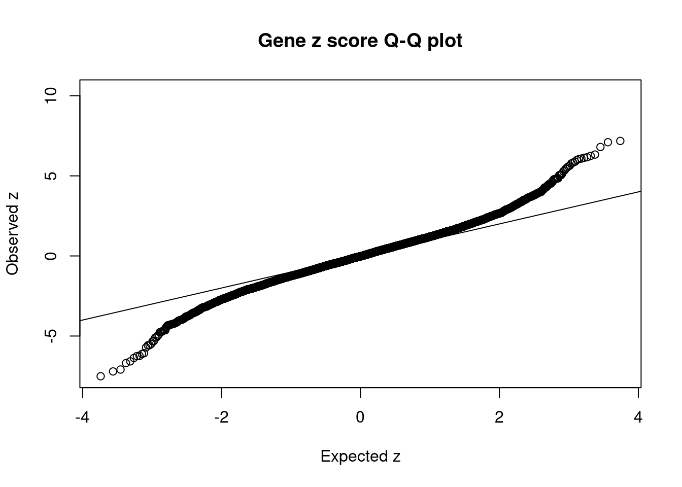
#plot z score vs PIP
plot(abs(ctwas_gene_res$z), ctwas_gene_res$susie_pip, xlab="abs(z)", ylab="PIP")
abline(v=sig_thresh, col="red", lty=2)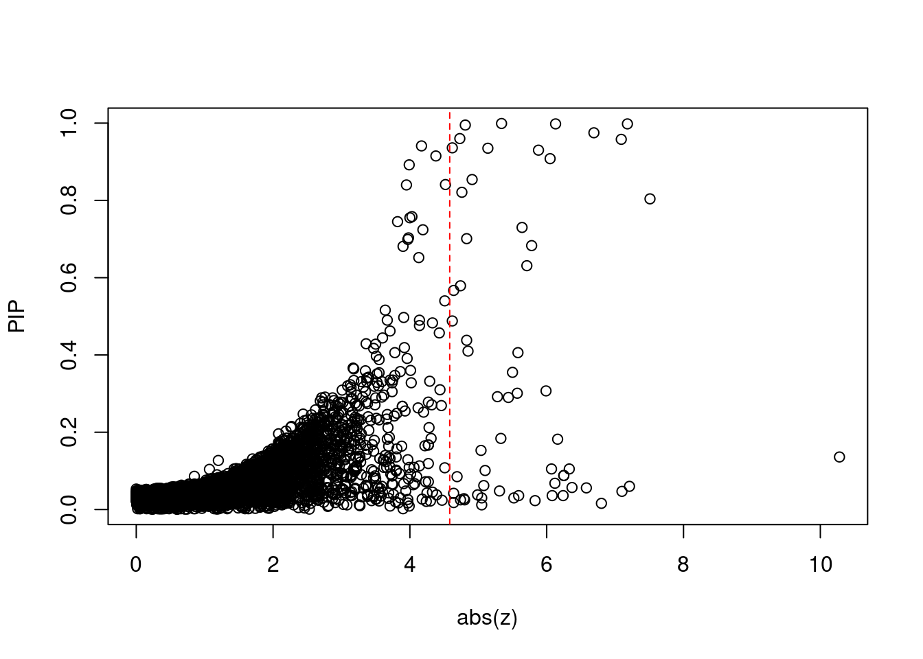
#proportion of significant z scores
mean(abs(ctwas_gene_res$z) > sig_thresh)
[1] 0.005516734#genes with most significant z scores
head(ctwas_gene_res[order(-abs(ctwas_gene_res$z)),report_cols],20) genename region_tag susie_pip mu2 PVE z
8651 MSL2 3_84 0.136 80.82 3.8e-05 10.28
537 DGAT2 11_42 0.804 49.68 1.4e-04 -7.51
11290 MAPKAPK5-AS1 12_66 0.060 39.97 8.1e-06 -7.21
12467 RP11-219B17.3 15_27 0.998 47.46 1.6e-04 7.18
2541 ALDH2 12_66 0.047 37.76 6.0e-06 7.10
1320 CWF19L1 10_64 0.958 30.61 1.0e-04 -7.09
2536 SH2B3 12_66 0.016 31.54 1.8e-06 6.80
10667 HLA-G 6_24 0.975 38.44 1.3e-04 -6.69
2170 AHR 7_17 0.056 45.73 8.7e-06 -6.58
4962 EXOC6 10_59 0.057 47.22 9.2e-06 -6.37
8505 HECTD4 12_66 0.105 35.90 1.3e-05 6.33
1191 ERP29 12_66 0.088 32.09 9.6e-06 6.25
10370 TMEM116 12_66 0.088 32.09 9.6e-06 -6.25
9829 ZKSCAN4 6_22 0.036 22.64 2.8e-06 -6.24
10425 AKR1C4 10_6 0.182 34.18 2.1e-05 6.16
1848 CD276 15_35 0.998 34.46 1.2e-04 6.13
2544 NAA25 12_66 0.068 29.70 6.9e-06 -6.12
3641 SLC17A1 6_20 0.036 47.50 5.8e-06 6.08
11216 CYP21A2 6_26 0.105 32.77 1.2e-05 -6.07
2924 EFHD1 2_136 0.908 37.25 1.2e-04 6.05Locus plots for genes and SNPs
ctwas_gene_res_sortz <- ctwas_gene_res[order(-abs(ctwas_gene_res$z)),]

n_plots <- 5
for (region_tag_plot in head(unique(ctwas_gene_res_sortz$region_tag), n_plots)){
  ctwas_res_region <-  ctwas_res[ctwas_res$region_tag==region_tag_plot,]
  start <- min(ctwas_res_region$pos)
  end <- max(ctwas_res_region$pos)

  ctwas_res_region <- ctwas_res_region[order(ctwas_res_region$pos),]
  ctwas_res_region_gene <- ctwas_res_region[ctwas_res_region$type=="gene",]
  ctwas_res_region_snp <- ctwas_res_region[ctwas_res_region$type=="SNP",]

  #region name
  print(paste0("Region: ", region_tag_plot))

  #table of genes in region
  print(ctwas_res_region_gene[,report_cols])

  par(mfrow=c(4,1))

  #gene z scores
  plot(ctwas_res_region_gene$pos, abs(ctwas_res_region_gene$z), xlab="Position", ylab="abs(gene_z)", xlim=c(start,end),
   ylim=c(0,max(sig_thresh, abs(ctwas_res_region_gene$z))),
   main=paste0("Region: ", region_tag_plot))
  abline(h=sig_thresh,col="red",lty=2)

  #significance threshold for SNPs
  alpha_snp <- 5*10^(-8)
  sig_thresh_snp <- qnorm(1-alpha_snp/2, lower=T)

  #snp z scores
  plot(ctwas_res_region_snp$pos, abs(ctwas_res_region_snp$z), xlab="Position", ylab="abs(snp_z)",xlim=c(start,end),
   ylim=c(0,max(sig_thresh_snp, max(abs(ctwas_res_region_snp$z)))))
  abline(h=sig_thresh_snp,col="purple",lty=2)

  #gene pips
  plot(ctwas_res_region_gene$pos, ctwas_res_region_gene$susie_pip, xlab="Position", ylab="Gene PIP", xlim=c(start,end), ylim=c(0,1))
  abline(h=0.8,col="blue",lty=2)

  #snp pips
  plot(ctwas_res_region_snp$pos, ctwas_res_region_snp$susie_pip, xlab="Position", ylab="SNP PIP", xlim=c(start,end), ylim=c(0,1))
  abline(h=0.8,col="blue",lty=2)
}
[1] "Region: 3_84"
genename region_tag susie_pip mu2 PVE z
796 PPP2R3A 3_84 0.069 13.42 3.2e-06 -2.46
8651 MSL2 3_84 0.136 80.82 3.8e-05 10.28
2795 PCCB 3_84 0.030 5.57 5.7e-07 1.22
3148 STAG1 3_84 0.033 5.11 5.7e-07 -0.03
6584 NCK1 3_84 0.030 7.87 8.1e-07 -2.19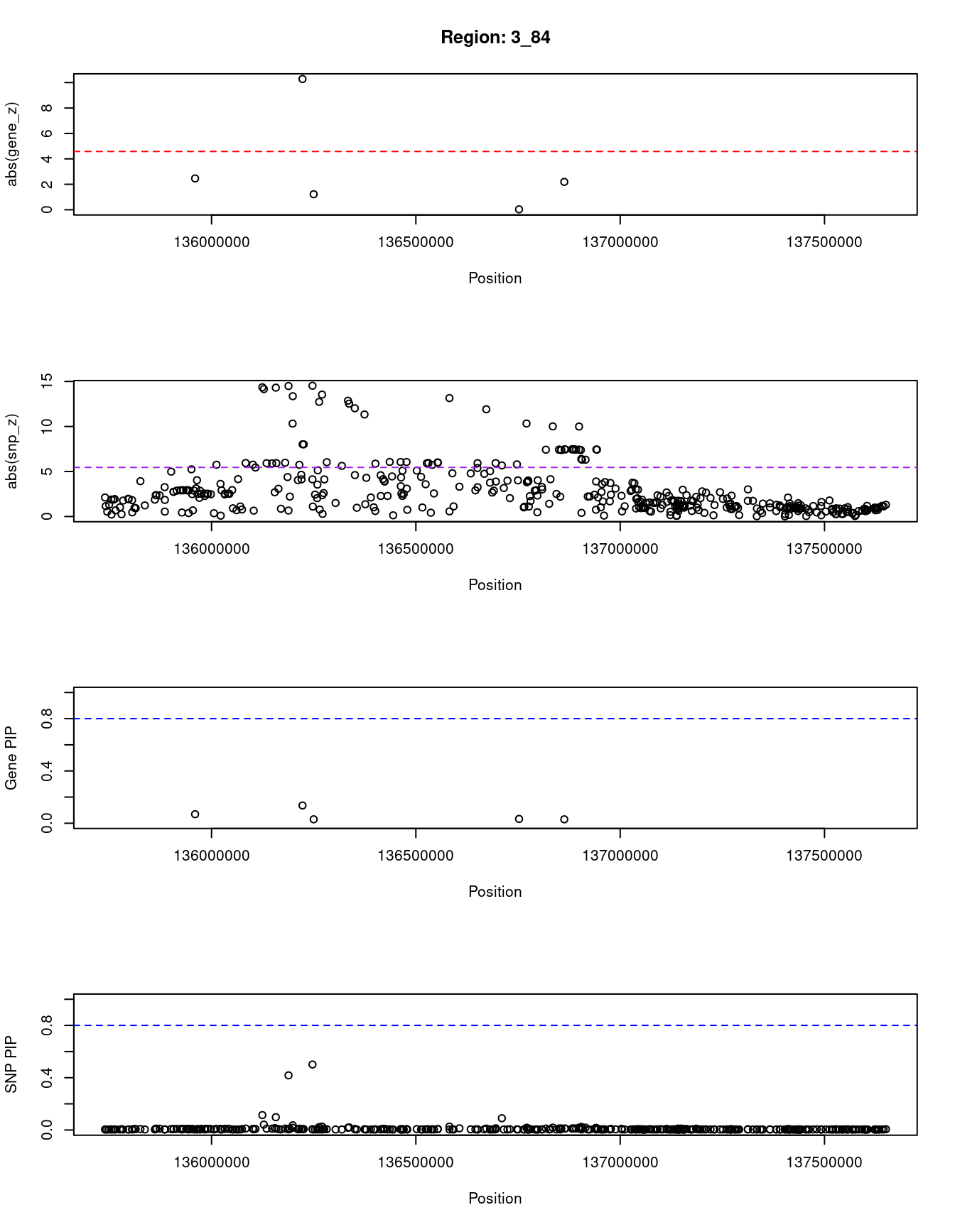
[1] "Region: 11_42"
           genename region_tag susie_pip   mu2     PVE     z
7611          XRRA1      11_42     0.031  8.09 8.5e-07 -1.00
3170          SPCS2      11_42     0.023  5.89 4.7e-07  0.73
6901           NEU3      11_42     0.021  4.64 3.3e-07  0.39
4848        SLCO2B1      11_42     0.021  4.65 3.3e-07 -0.22
12001         TPBGL      11_42     0.028  7.28 7.0e-07  0.68
6617          GDPD5      11_42     0.032 10.58 1.1e-06  1.95
8328           MAP6      11_42     0.025  6.11 5.2e-07  0.24
7603         MOGAT2      11_42     0.086 15.16 4.5e-06  0.85
537           DGAT2      11_42     0.804 49.68 1.4e-04 -7.51
10381         UVRAG      11_42     0.024  6.88 5.6e-07  1.62
1082          WNT11      11_42     0.030  7.98 8.0e-07  1.06
11773 RP11-619A14.3      11_42     0.024  5.82 4.7e-07  0.61
4849         THAP12      11_42     0.022  5.44 4.1e-07 -0.66
12265 RP11-111M22.5      11_42     0.025  6.37 5.4e-07  0.80
11766 RP11-111M22.3      11_42     0.021  4.69 3.3e-07  0.31
11751  RP11-672A2.4      11_42     0.022  5.37 4.1e-07  0.53
9350           TSKU      11_42     0.022  5.00 3.7e-07  0.25
905           ACER3      11_42     0.081 16.62 4.6e-06 -2.04
5976          CAPN5      11_42     0.056 13.67 2.6e-06  1.72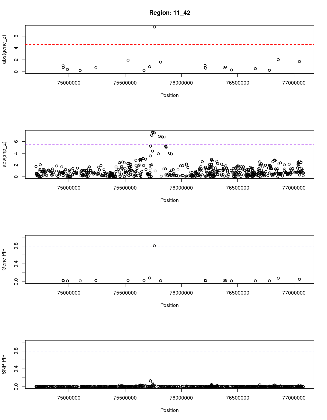
[1] "Region: 12_66"
          genename region_tag susie_pip   mu2     PVE     z
5112          TCHP      12_66     0.217 16.64 1.2e-05  3.21
5111          GIT2      12_66     0.143 15.95 7.8e-06  3.36
8639      C12orf76      12_66     0.016  6.20 3.4e-07 -0.30
3515         IFT81      12_66     0.020 11.38 7.9e-07  2.50
10093       ANAPC7      12_66     0.020  9.13 6.3e-07  2.16
2531         ARPC3      12_66     0.019  7.35 4.9e-07  0.54
10684      FAM216A      12_66     0.018  9.95 6.0e-07  2.42
2532          GPN3      12_66     0.014  5.66 2.6e-07  1.40
2533         VPS29      12_66     0.014  5.73 2.7e-07 -1.41
10683        TCTN1      12_66     0.017  5.93 3.3e-07  0.02
3517         HVCN1      12_66     0.034 14.22 1.6e-06  2.67
9717        PPP1CC      12_66     0.034 14.14 1.6e-06 -2.65
10375      FAM109A      12_66     0.014  7.61 3.7e-07 -1.46
2536         SH2B3      12_66     0.016 31.54 1.8e-06  6.80
10680        ATXN2      12_66     0.017 20.43 1.2e-06  3.97
2541         ALDH2      12_66     0.047 37.76 6.0e-06  7.10
11290 MAPKAPK5-AS1      12_66     0.060 39.97 8.1e-06 -7.21
1191         ERP29      12_66     0.088 32.09 9.6e-06  6.25
10370      TMEM116      12_66     0.088 32.09 9.6e-06 -6.25
2544         NAA25      12_66     0.068 29.70 6.9e-06 -6.12
8505        HECTD4      12_66     0.105 35.90 1.3e-05  6.33
9084        PTPN11      12_66     0.016  6.36 3.5e-07 -0.78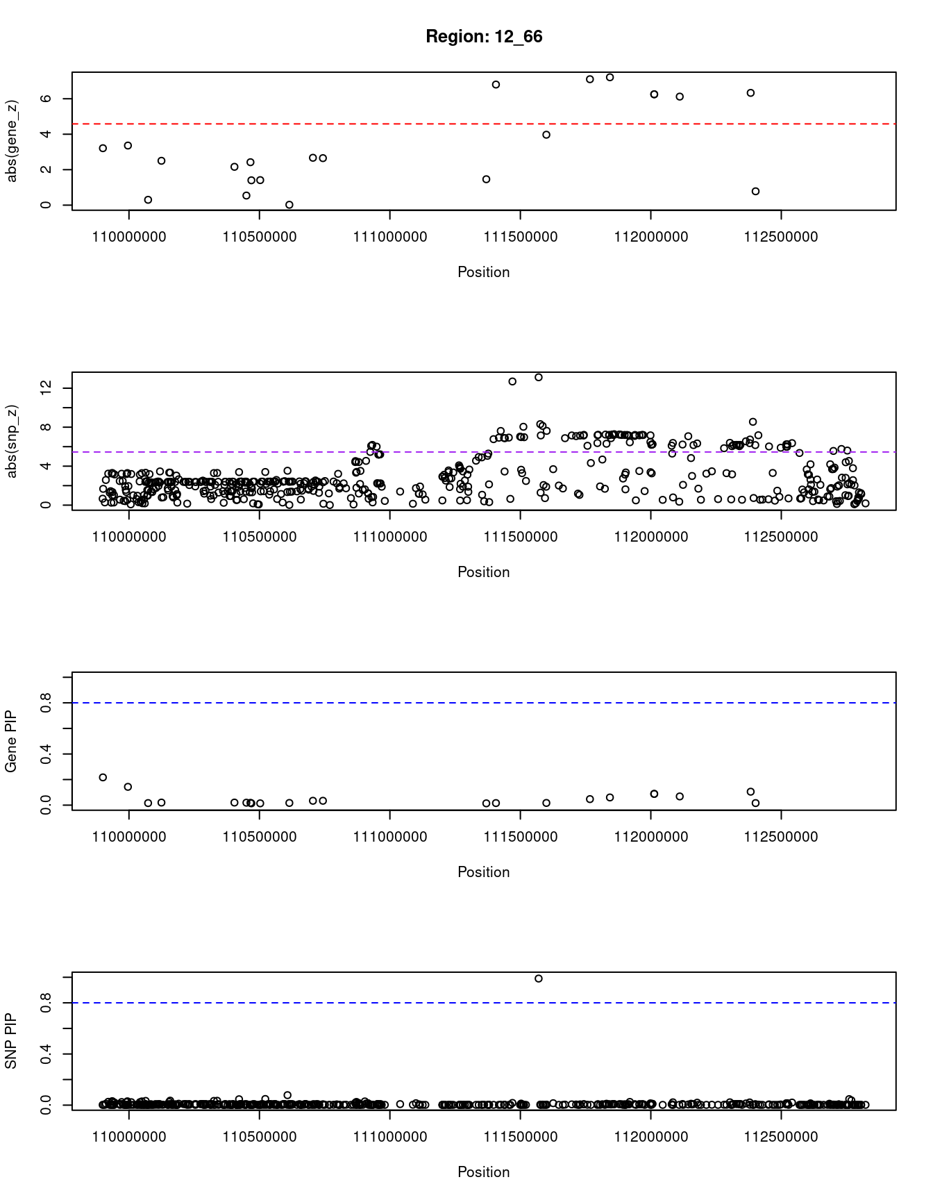
[1] "Region: 15_27"
           genename region_tag susie_pip   mu2     PVE     z
5185          GCNT3      15_27     0.037  6.23 7.9e-07 -0.60
5186         GTF2A2      15_27     0.054  9.58 1.8e-06 -1.23
3965           ICE2      15_27     0.031  6.67 7.1e-07 -1.54
12467 RP11-219B17.3      15_27     0.998 47.46 1.6e-04  7.18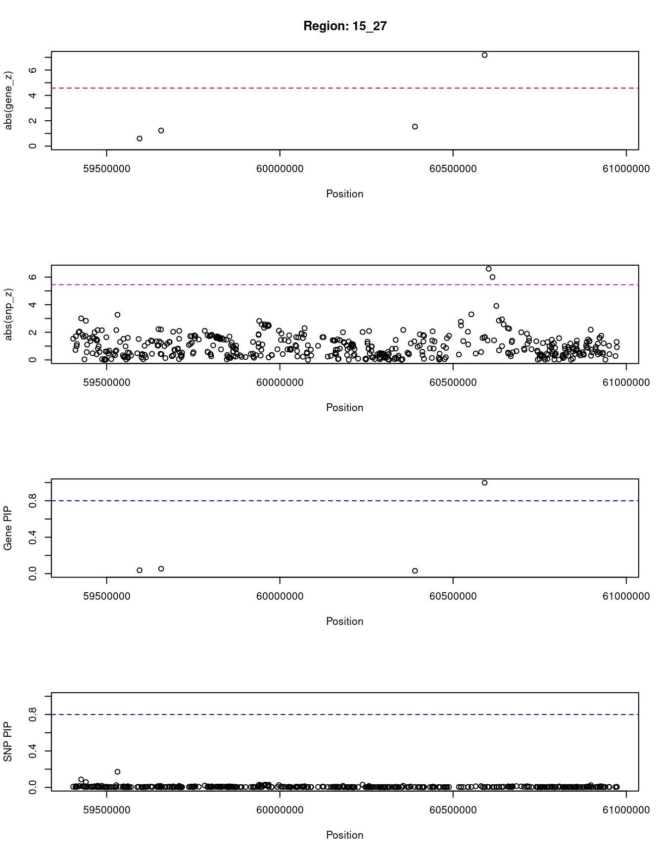
[1] "Region: 10_64"
           genename region_tag susie_pip   mu2     PVE     z
3299          CNNM1      10_64     0.041 17.81 2.5e-06  2.68
3307           GOT1      10_64     0.039 19.82 2.7e-06  3.38
11056 RP11-441O15.3      10_64     0.039 19.82 2.7e-06 -3.38
11947   RP11-85A1.3      10_64     0.015  7.57 3.8e-07 -0.63
10330        ENTPD7      10_64     0.012  6.60 2.7e-07  0.21
3296           CUTC      10_64     0.013  7.36 3.3e-07  0.46
228           COX15      10_64     0.011  5.10 2.0e-07  0.08
281           ABCC2      10_64     0.030 24.03 2.5e-06  5.05
2234          DNMBP      10_64     0.037 20.06 2.5e-06 -3.13
3308           CPN1      10_64     0.012 12.43 5.1e-07  5.05
2237         ERLIN1      10_64     0.019 13.48 8.9e-07 -2.74
10819          CHUK      10_64     0.014  7.59 3.5e-07 -1.62
1320        CWF19L1      10_64     0.958 30.61 1.0e-04 -7.09
10014       BLOC1S2      10_64     0.017 10.87 6.3e-07 -2.24
11326      OLMALINC      10_64     0.019 11.22 7.1e-07 -2.01
12405 RP11-285F16.1      10_64     0.013  5.91 2.7e-07 -0.59
7557         NDUFB8      10_64     0.015  6.55 3.3e-07 -0.61
3291           SLF2      10_64     0.012  5.01 2.0e-07 -0.49
1321         SEMA4G      10_64     0.022 10.30 7.9e-07 -1.03
2256          LZTS2      10_64     0.012  4.87 2.0e-07  0.03
9772          PDZD7      10_64     0.025 11.14 9.4e-07  1.21
2254           TLX1      10_64     0.021  9.99 7.1e-07  1.04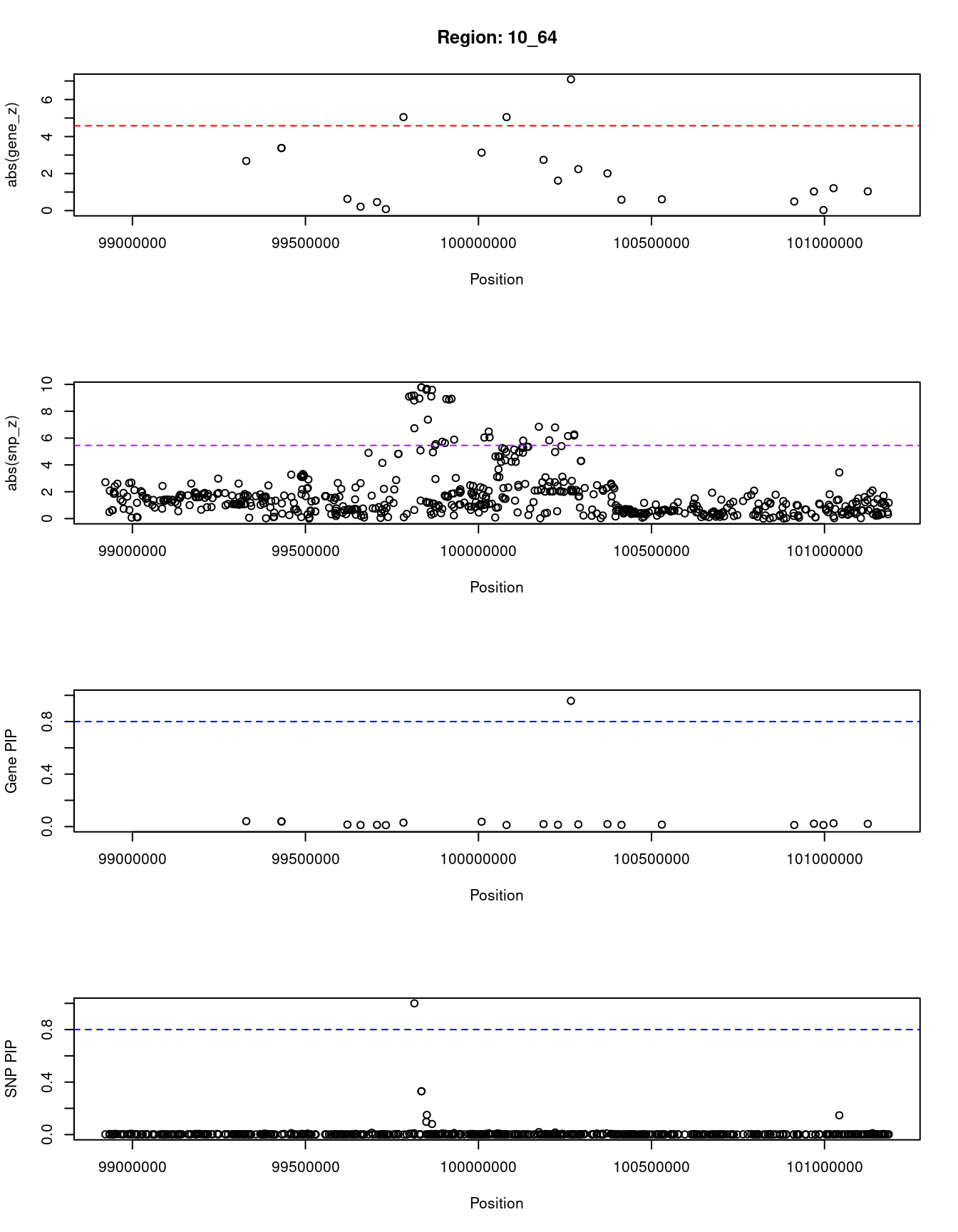
SNPs with highest PIPs
#snps with PIP>0.8 or 20 highest PIPs
head(ctwas_snp_res[order(-ctwas_snp_res$susie_pip),report_cols_snps],
max(sum(ctwas_snp_res$susie_pip>0.8), 20))
id region_tag susie_pip mu2 PVE z
330793 rs72834643 6_20 1.000 94.30 3.2e-04 9.73
330814 rs115740542 6_20 1.000 143.95 4.9e-04 12.66
376219 rs12208357 6_103 1.000 60.36 2.1e-04 -6.65
388005 rs542176135 7_17 1.000 100.83 3.4e-04 -8.38
539954 rs6480402 10_46 1.000 155.90 5.3e-04 8.90
549432 rs111286300 10_64 1.000 34.49 1.2e-04 6.73
811047 rs59616136 19_14 1.000 41.67 1.4e-04 7.00
136166 rs6731991 2_136 0.999 33.88 1.2e-04 -5.75
539953 rs4745982 10_46 0.999 60.61 2.1e-04 11.95
331984 rs3130253 6_23 0.998 34.34 1.2e-04 -6.63
819540 rs113345881 19_32 0.998 32.30 1.1e-04 6.12
515241 rs115478735 9_70 0.997 53.75 1.8e-04 -8.02
819538 rs814573 19_32 0.996 33.75 1.1e-04 -6.68
561859 rs76153913 11_2 0.994 41.04 1.4e-04 6.70
831269 rs34507316 20_13 0.991 27.41 9.3e-05 5.60
637833 rs653178 12_66 0.990 130.44 4.4e-04 -13.12
621249 rs7397189 12_35 0.987 29.65 1.0e-04 5.69
809276 rs141645070 19_10 0.977 26.33 8.8e-05 -5.27
756467 rs2608604 16_53 0.966 40.34 1.3e-04 -6.33
37561 rs2779116 1_78 0.963 58.83 1.9e-04 -8.25
819543 rs12721109 19_32 0.957 29.11 9.5e-05 6.44
716804 rs2070895 15_26 0.941 27.90 9.0e-05 -5.24
819474 rs1551891 19_32 0.935 33.76 1.1e-04 7.88
539974 rs73267649 10_46 0.932 63.74 2.0e-04 -3.84
811832 rs3794991 19_15 0.931 107.07 3.4e-04 11.64
611249 rs73080739 12_15 0.922 31.25 9.8e-05 -7.24
860343 rs34662558 22_10 0.907 26.45 8.2e-05 -5.19
515626 rs34755157 9_71 0.905 25.20 7.8e-05 -5.03
611244 rs7962574 12_15 0.903 42.83 1.3e-04 -8.40
566312 rs34623292 11_10 0.897 25.87 7.9e-05 -5.06
388027 rs4721597 7_17 0.896 47.67 1.5e-04 1.94
237701 rs17238095 4_72 0.886 26.69 8.1e-05 5.18
501160 rs9410381 9_45 0.872 63.49 1.9e-04 8.62
443676 rs12549737 8_24 0.845 26.32 7.6e-05 5.15
673588 rs35115456 13_53 0.815 24.34 6.8e-05 -4.47
863094 rs6000553 22_14 0.814 37.48 1.0e-04 6.47
611284 rs10770693 12_15 0.813 53.50 1.5e-04 8.86
299010 rs4566840 5_66 0.808 27.05 7.5e-05 -5.46
564881 rs4910498 11_8 0.803 43.52 1.2e-04 6.71SNPs with largest effect sizes
#plot PIP vs effect size
plot(ctwas_snp_res$susie_pip, ctwas_snp_res$mu2, xlab="PIP", ylab="mu^2", main="SNP PIPs vs Effect Size")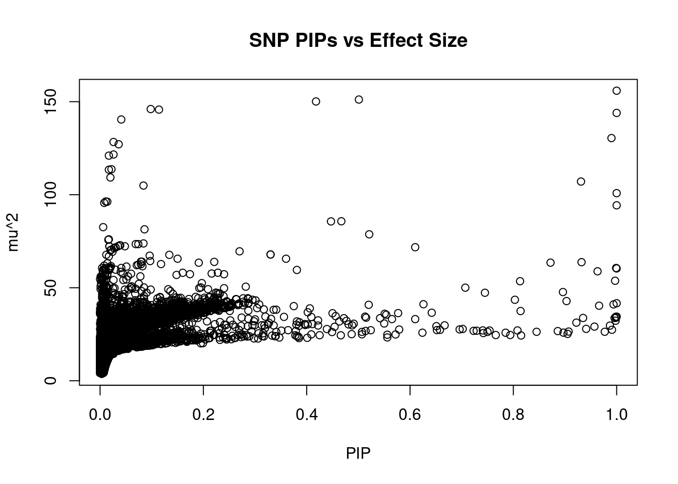
#SNPs with 50 largest effect sizes
head(ctwas_snp_res[order(-ctwas_snp_res$mu2),report_cols_snps],50)
id region_tag susie_pip mu2 PVE z
539954 rs6480402 10_46 1.000 155.90 5.3e-04 8.90
181216 rs523118 3_84 0.501 151.15 2.6e-04 -14.52
181205 rs6779146 3_84 0.418 150.11 2.1e-04 14.49
181198 rs9865841 3_84 0.098 146.03 4.9e-05 -14.31
181193 rs9840812 3_84 0.114 145.74 5.7e-05 -14.35
330814 rs115740542 6_20 1.000 143.95 4.9e-04 12.66
181194 rs2400727 3_84 0.041 140.43 1.9e-05 -14.15
637833 rs653178 12_66 0.990 130.44 4.4e-04 -13.12
181224 rs576771 3_84 0.026 128.33 1.1e-05 -13.54
181208 rs61789561 3_84 0.036 127.11 1.5e-05 13.36
181274 rs12630999 3_84 0.026 121.61 1.1e-05 -13.15
637825 rs35350651 12_66 0.017 121.00 6.8e-06 -12.69
181222 rs372863955 3_84 0.022 113.69 8.5e-06 -12.73
181232 rs610860 3_84 0.017 113.45 6.8e-06 -12.86
181233 rs8045 3_84 0.020 109.26 7.6e-06 12.53
811832 rs3794991 19_15 0.931 107.07 3.4e-04 11.64
811858 rs73004951 19_15 0.084 104.92 3.0e-05 11.37
388005 rs542176135 7_17 1.000 100.83 3.4e-04 -8.38
181285 rs3856637 3_84 0.011 96.36 3.7e-06 11.91
388014 rs10950655 7_17 0.014 96.24 4.8e-06 -7.96
181234 rs667920 3_84 0.008 95.60 2.5e-06 -12.02
330793 rs72834643 6_20 1.000 94.30 3.2e-04 9.73
539959 rs35233497 10_46 0.467 85.72 1.4e-04 -4.24
539962 rs79086908 10_46 0.447 85.64 1.3e-04 -4.24
181237 rs35923792 3_84 0.006 82.56 1.6e-06 -11.33
539960 rs570124086 10_46 0.086 81.40 2.4e-05 -4.08
537908 rs7090758 10_42 0.521 78.71 1.4e-04 9.99
181207 rs35087366 3_84 0.017 76.02 4.4e-06 10.32
181300 rs71336078 3_84 0.016 75.76 4.2e-06 10.33
537911 rs10822186 10_42 0.084 73.81 2.1e-05 -9.73
537910 rs570234162 10_42 0.069 73.44 1.7e-05 9.70
537912 rs7895549 10_42 0.074 73.44 1.9e-05 -9.71
537811 rs1935 10_42 0.039 72.80 9.7e-06 -9.60
537806 rs35751397 10_42 0.038 72.77 9.4e-06 -9.59
537854 rs10822160 10_42 0.035 72.32 8.7e-06 -9.58
537903 rs2163188 10_42 0.048 72.29 1.2e-05 9.65
181318 rs1406539 3_84 0.018 72.25 4.4e-06 -10.01
181333 rs370148911 3_84 0.018 72.23 4.5e-06 -9.99
502009 rs7849152 9_46 0.610 71.78 1.5e-04 9.47
537822 rs10761729 10_42 0.030 71.71 7.4e-06 -9.55
537866 rs10822168 10_42 0.030 71.63 7.3e-06 -9.55
537860 rs7910927 10_42 0.027 71.25 6.6e-06 -9.54
537875 rs3956912 10_42 0.027 71.24 6.6e-06 -9.54
537842 rs5785566 10_42 0.022 70.50 5.3e-06 -9.50
537858 rs6479896 10_42 0.021 70.24 5.1e-06 -9.49
537868 rs10640079 10_42 0.020 70.10 4.8e-06 -9.49
502023 rs111550777 9_46 0.270 69.57 6.4e-05 9.36
537907 rs4746205 10_42 0.024 69.31 5.8e-06 9.56
549436 rs55672373 10_64 0.330 67.87 7.7e-05 -9.78
549437 rs55804858 10_64 0.330 67.86 7.6e-05 -9.78SNPs with highest PVE
#SNPs with 50 highest pve
head(ctwas_snp_res[order(-ctwas_snp_res$PVE),report_cols_snps],50)
id region_tag susie_pip mu2 PVE z
539954 rs6480402 10_46 1.000 155.90 5.3e-04 8.90
330814 rs115740542 6_20 1.000 143.95 4.9e-04 12.66
637833 rs653178 12_66 0.990 130.44 4.4e-04 -13.12
388005 rs542176135 7_17 1.000 100.83 3.4e-04 -8.38
811832 rs3794991 19_15 0.931 107.07 3.4e-04 11.64
330793 rs72834643 6_20 1.000 94.30 3.2e-04 9.73
181216 rs523118 3_84 0.501 151.15 2.6e-04 -14.52
181205 rs6779146 3_84 0.418 150.11 2.1e-04 14.49
376219 rs12208357 6_103 1.000 60.36 2.1e-04 -6.65
539953 rs4745982 10_46 0.999 60.61 2.1e-04 11.95
539974 rs73267649 10_46 0.932 63.74 2.0e-04 -3.84
37561 rs2779116 1_78 0.963 58.83 1.9e-04 -8.25
501160 rs9410381 9_45 0.872 63.49 1.9e-04 8.62
515241 rs115478735 9_70 0.997 53.75 1.8e-04 -8.02
388027 rs4721597 7_17 0.896 47.67 1.5e-04 1.94
502009 rs7849152 9_46 0.610 71.78 1.5e-04 9.47
611284 rs10770693 12_15 0.813 53.50 1.5e-04 8.86
537908 rs7090758 10_42 0.521 78.71 1.4e-04 9.99
539959 rs35233497 10_46 0.467 85.72 1.4e-04 -4.24
561859 rs76153913 11_2 0.994 41.04 1.4e-04 6.70
811047 rs59616136 19_14 1.000 41.67 1.4e-04 7.00
539962 rs79086908 10_46 0.447 85.64 1.3e-04 -4.24
611244 rs7962574 12_15 0.903 42.83 1.3e-04 -8.40
756467 rs2608604 16_53 0.966 40.34 1.3e-04 -6.33
136166 rs6731991 2_136 0.999 33.88 1.2e-04 -5.75
330632 rs75080831 6_19 0.707 50.03 1.2e-04 7.96
331984 rs3130253 6_23 0.998 34.34 1.2e-04 -6.63
549432 rs111286300 10_64 1.000 34.49 1.2e-04 6.73
561905 rs16929046 11_2 0.745 47.30 1.2e-04 7.10
564881 rs4910498 11_8 0.803 43.52 1.2e-04 6.71
819474 rs1551891 19_32 0.935 33.76 1.1e-04 7.88
819538 rs814573 19_32 0.996 33.75 1.1e-04 -6.68
819540 rs113345881 19_32 0.998 32.30 1.1e-04 6.12
621249 rs7397189 12_35 0.987 29.65 1.0e-04 5.69
863094 rs6000553 22_14 0.814 37.48 1.0e-04 6.47
611249 rs73080739 12_15 0.922 31.25 9.8e-05 -7.24
819543 rs12721109 19_32 0.957 29.11 9.5e-05 6.44
831269 rs34507316 20_13 0.991 27.41 9.3e-05 5.60
716804 rs2070895 15_26 0.941 27.90 9.0e-05 -5.24
376232 rs1443844 6_103 0.626 41.14 8.8e-05 4.37
809276 rs141645070 19_10 0.977 26.33 8.8e-05 -5.27
860343 rs34662558 22_10 0.907 26.45 8.2e-05 -5.19
237701 rs17238095 4_72 0.886 26.69 8.1e-05 5.18
547440 rs570762793 10_59 0.360 65.59 8.1e-05 9.01
334157 rs9267293 6_25 0.642 36.56 8.0e-05 -6.54
566312 rs34623292 11_10 0.897 25.87 7.9e-05 -5.06
515626 rs34755157 9_71 0.905 25.20 7.8e-05 -5.03
549436 rs55672373 10_64 0.330 67.87 7.7e-05 -9.78
555752 rs7078330 10_75 0.381 59.56 7.7e-05 -8.30
443676 rs12549737 8_24 0.845 26.32 7.6e-05 5.15SNPs with largest z scores
#SNPs with 50 largest z scores
head(ctwas_snp_res[order(-abs(ctwas_snp_res$z)),report_cols_snps],50)
id region_tag susie_pip mu2 PVE z
181216 rs523118 3_84 0.501 151.15 2.6e-04 -14.52
181205 rs6779146 3_84 0.418 150.11 2.1e-04 14.49
181193 rs9840812 3_84 0.114 145.74 5.7e-05 -14.35
181198 rs9865841 3_84 0.098 146.03 4.9e-05 -14.31
181194 rs2400727 3_84 0.041 140.43 1.9e-05 -14.15
181224 rs576771 3_84 0.026 128.33 1.1e-05 -13.54
181208 rs61789561 3_84 0.036 127.11 1.5e-05 13.36
181274 rs12630999 3_84 0.026 121.61 1.1e-05 -13.15
637833 rs653178 12_66 0.990 130.44 4.4e-04 -13.12
181232 rs610860 3_84 0.017 113.45 6.8e-06 -12.86
181222 rs372863955 3_84 0.022 113.69 8.5e-06 -12.73
637825 rs35350651 12_66 0.017 121.00 6.8e-06 -12.69
330814 rs115740542 6_20 1.000 143.95 4.9e-04 12.66
181233 rs8045 3_84 0.020 109.26 7.6e-06 12.53
181234 rs667920 3_84 0.008 95.60 2.5e-06 -12.02
539953 rs4745982 10_46 0.999 60.61 2.1e-04 11.95
181285 rs3856637 3_84 0.011 96.36 3.7e-06 11.91
811832 rs3794991 19_15 0.931 107.07 3.4e-04 11.64
811858 rs73004951 19_15 0.084 104.92 3.0e-05 11.37
181237 rs35923792 3_84 0.006 82.56 1.6e-06 -11.33
181300 rs71336078 3_84 0.016 75.76 4.2e-06 10.33
181207 rs35087366 3_84 0.017 76.02 4.4e-06 10.32
181318 rs1406539 3_84 0.018 72.25 4.4e-06 -10.01
330804 rs1800702 6_20 0.011 60.03 2.2e-06 10.00
181333 rs370148911 3_84 0.018 72.23 4.5e-06 -9.99
330801 rs7738854 6_20 0.010 59.34 2.1e-06 9.99
537908 rs7090758 10_42 0.521 78.71 1.4e-04 9.99
330799 rs9348706 6_20 0.010 58.09 1.9e-06 9.94
330786 rs2032449 6_20 0.009 56.41 1.7e-06 9.87
549436 rs55672373 10_64 0.330 67.87 7.7e-05 -9.78
549437 rs55804858 10_64 0.330 67.86 7.6e-05 -9.78
330793 rs72834643 6_20 1.000 94.30 3.2e-04 9.73
330795 rs2032446 6_20 0.008 54.13 1.4e-06 9.73
537911 rs10822186 10_42 0.084 73.81 2.1e-05 -9.73
537912 rs7895549 10_42 0.074 73.44 1.9e-05 -9.71
537910 rs570234162 10_42 0.069 73.44 1.7e-05 9.70
549440 rs17216212 10_64 0.150 65.59 3.4e-05 -9.67
537903 rs2163188 10_42 0.048 72.29 1.2e-05 9.65
537811 rs1935 10_42 0.039 72.80 9.7e-06 -9.60
537806 rs35751397 10_42 0.038 72.77 9.4e-06 -9.59
549439 rs72838143 10_64 0.097 64.34 2.1e-05 -9.59
549447 rs113354025 10_64 0.081 64.00 1.8e-05 -9.59
537854 rs10822160 10_42 0.035 72.32 8.7e-06 -9.58
537907 rs4746205 10_42 0.024 69.31 5.8e-06 9.56
537822 rs10761729 10_42 0.030 71.71 7.4e-06 -9.55
537866 rs10822168 10_42 0.030 71.63 7.3e-06 -9.55
537860 rs7910927 10_42 0.027 71.25 6.6e-06 -9.54
537875 rs3956912 10_42 0.027 71.24 6.6e-06 -9.54
537842 rs5785566 10_42 0.022 70.50 5.3e-06 -9.50
537858 rs6479896 10_42 0.021 70.24 5.1e-06 -9.49
sessionInfo()R version 4.1.0 (2021-05-18)
Platform: x86_64-pc-linux-gnu (64-bit)
Running under: CentOS Linux 7 (Core)
Matrix products: default
BLAS: /software/R-4.1.0-no-openblas-el7-x86_64/lib64/R/lib/libRblas.so
LAPACK: /software/R-4.1.0-no-openblas-el7-x86_64/lib64/R/lib/libRlapack.so
locale:
[1] LC_CTYPE=en_US.UTF-8 LC_NUMERIC=C LC_TIME=C
[4] LC_COLLATE=C LC_MONETARY=C LC_MESSAGES=C
[7] LC_PAPER=C LC_NAME=C LC_ADDRESS=C
[10] LC_TELEPHONE=C LC_MEASUREMENT=C LC_IDENTIFICATION=C
attached base packages:
[1] stats graphics grDevices utils datasets methods base
other attached packages:
[1] cowplot_1.1.1 ggplot2_3.4.0
loaded via a namespace (and not attached):
[1] bitops_1.0-7 matrixStats_0.63.0
[3] fs_1.5.2 bit64_4.0.5
[5] filelock_1.0.2 progress_1.2.2
[7] httr_1.4.4 rprojroot_2.0.3
[9] GenomeInfoDb_1.30.1 tools_4.1.0
[11] bslib_0.4.1 utf8_1.2.2
[13] R6_2.5.1 colorspace_2.0-3
[15] DBI_1.1.3 BiocGenerics_0.40.0
[17] withr_2.5.0 tidyselect_1.2.0
[19] prettyunits_1.1.1 bit_4.0.5
[21] curl_4.3.3 compiler_4.1.0
[23] git2r_0.30.1 cli_3.4.1
[25] Biobase_2.54.0 xml2_1.3.3
[27] DelayedArray_0.20.0 labeling_0.4.2
[29] rtracklayer_1.54.0 sass_0.4.4
[31] scales_1.2.1 rappdirs_0.3.3
[33] stringr_1.5.0 digest_0.6.31
[35] Rsamtools_2.10.0 rmarkdown_2.18
[37] XVector_0.34.0 pkgconfig_2.0.3
[39] htmltools_0.5.4 MatrixGenerics_1.6.0
[41] highr_0.9 dbplyr_2.2.1
[43] fastmap_1.1.0 BSgenome_1.62.0
[45] rlang_1.0.6 rstudioapi_0.14
[47] RSQLite_2.2.19 farver_2.1.1
[49] jquerylib_0.1.4 BiocIO_1.4.0
[51] generics_0.1.3 jsonlite_1.8.4
[53] BiocParallel_1.28.3 dplyr_1.0.10
[55] VariantAnnotation_1.40.0 RCurl_1.98-1.9
[57] magrittr_2.0.3 GenomeInfoDbData_1.2.7
[59] Matrix_1.5-3 munsell_0.5.0
[61] Rcpp_1.0.9 S4Vectors_0.32.4
[63] fansi_1.0.3 lifecycle_1.0.3
[65] stringi_1.7.8 whisker_0.4.1
[67] yaml_2.3.6 SummarizedExperiment_1.24.0
[69] zlibbioc_1.40.0 BiocFileCache_2.2.1
[71] grid_4.1.0 blob_1.2.3
[73] parallel_4.1.0 promises_1.2.0.1
[75] crayon_1.5.2 lattice_0.20-45
[77] Biostrings_2.62.0 GenomicFeatures_1.46.5
[79] hms_1.1.2 KEGGREST_1.34.0
[81] knitr_1.41 pillar_1.8.1
[83] GenomicRanges_1.46.1 rjson_0.2.21
[85] biomaRt_2.50.3 stats4_4.1.0
[87] XML_3.99-0.13 glue_1.6.2
[89] evaluate_0.18 data.table_1.14.6
[91] png_0.1-8 vctrs_0.5.1
[93] httpuv_1.6.6 gtable_0.3.1
[95] assertthat_0.2.1 cachem_1.0.6
[97] xfun_0.35 restfulr_0.0.15
[99] later_1.3.0 tibble_3.1.8
[101] GenomicAlignments_1.30.0 AnnotationDbi_1.56.2
[103] memoise_2.0.1 IRanges_2.28.0
[105] workflowr_1.7.0 ellipsis_0.3.2