Direct bilirubin (quantile) - Liver [fixed prior variance]
wesleycrouse
2021-08-18
Last updated: 2021-09-09
Checks: 7 0
Knit directory: ctwas_applied/
This reproducible R Markdown analysis was created with workflowr (version 1.6.2). The Checks tab describes the reproducibility checks that were applied when the results were created. The Past versions tab lists the development history.
Great! Since the R Markdown file has been committed to the Git repository, you know the exact version of the code that produced these results.
Great job! The global environment was empty. Objects defined in the global environment can affect the analysis in your R Markdown file in unknown ways. For reproduciblity it’s best to always run the code in an empty environment.
The command set.seed(20210726) was run prior to running the code in the R Markdown file. Setting a seed ensures that any results that rely on randomness, e.g. subsampling or permutations, are reproducible.
Great job! Recording the operating system, R version, and package versions is critical for reproducibility.
Nice! There were no cached chunks for this analysis, so you can be confident that you successfully produced the results during this run.
Great job! Using relative paths to the files within your workflowr project makes it easier to run your code on other machines.
Great! You are using Git for version control. Tracking code development and connecting the code version to the results is critical for reproducibility.
The results in this page were generated with repository version 59e5f4d. See the Past versions tab to see a history of the changes made to the R Markdown and HTML files.
Note that you need to be careful to ensure that all relevant files for the analysis have been committed to Git prior to generating the results (you can use wflow_publish or wflow_git_commit). workflowr only checks the R Markdown file, but you know if there are other scripts or data files that it depends on. Below is the status of the Git repository when the results were generated:
Unstaged changes:
    Modified:   analysis/ukb-d-30500_irnt_Liver.Rmd
    Modified:   analysis/ukb-d-30500_irnt_Whole_Blood.Rmd
    Modified:   analysis/ukb-d-30600_irnt_Liver.Rmd
    Modified:   analysis/ukb-d-30600_irnt_Whole_Blood.Rmd
    Modified:   analysis/ukb-d-30610_irnt_Liver.Rmd
    Modified:   analysis/ukb-d-30610_irnt_Whole_Blood.Rmd
    Modified:   analysis/ukb-d-30620_irnt_Liver.Rmd
    Modified:   analysis/ukb-d-30620_irnt_Whole_Blood.Rmd
    Modified:   analysis/ukb-d-30630_irnt_Liver.Rmd
    Modified:   analysis/ukb-d-30630_irnt_Whole_Blood.Rmd
    Modified:   analysis/ukb-d-30640_irnt_Liver.Rmd
    Modified:   analysis/ukb-d-30640_irnt_Whole_Blood.Rmd
    Modified:   analysis/ukb-d-30650_irnt_Liver.Rmd
    Modified:   analysis/ukb-d-30650_irnt_Whole_Blood.Rmd
    Modified:   analysis/ukb-d-30660_irnt_Liver.Rmd
    Modified:   analysis/ukb-d-30660_irnt_Whole_Blood.Rmd
    Modified:   analysis/ukb-d-30670_irnt_Liver.Rmd
    Modified:   analysis/ukb-d-30670_irnt_Whole_Blood.Rmd
    Modified:   analysis/ukb-d-30680_irnt_Liver.Rmd
    Modified:   analysis/ukb-d-30690_irnt_Liver.Rmd
    Modified:   analysis/ukb-d-30690_irnt_Whole_Blood.Rmd
    Modified:   analysis/ukb-d-30700_irnt_Liver.Rmd
    Modified:   analysis/ukb-d-30700_irnt_Whole_Blood.Rmd
    Modified:   analysis/ukb-d-30710_irnt_Liver.Rmd
    Modified:   analysis/ukb-d-30710_irnt_Whole_Blood.Rmd
    Modified:   analysis/ukb-d-30720_irnt_Liver.Rmd
    Modified:   analysis/ukb-d-30720_irnt_Whole_Blood.Rmd
    Modified:   analysis/ukb-d-30730_irnt_Liver.Rmd
    Modified:   analysis/ukb-d-30740_irnt_Liver.Rmd
    Modified:   analysis/ukb-d-30740_irnt_Whole_Blood.Rmd
    Modified:   analysis/ukb-d-30750_irnt_Liver.Rmd
    Modified:   analysis/ukb-d-30750_irnt_Whole_Blood.Rmd
    Modified:   analysis/ukb-d-30760_irnt_Liver.Rmd
    Modified:   analysis/ukb-d-30760_irnt_Whole_Blood.Rmd
    Modified:   analysis/ukb-d-30770_irnt_Liver.Rmd
    Modified:   analysis/ukb-d-30770_irnt_Whole_Blood.Rmd
    Modified:   analysis/ukb-d-30780_irnt_Liver.Rmd
    Modified:   analysis/ukb-d-30780_irnt_Whole_Blood.Rmd
    Modified:   analysis/ukb-d-30790_irnt_Liver.Rmd
    Modified:   analysis/ukb-d-30800_irnt_Liver.Rmd
    Modified:   analysis/ukb-d-30800_irnt_Whole_Blood.Rmd
    Modified:   analysis/ukb-d-30810_irnt_Liver.Rmd
    Modified:   analysis/ukb-d-30820_irnt_Liver.Rmd
    Modified:   analysis/ukb-d-30820_irnt_Whole_Blood.Rmd
    Modified:   analysis/ukb-d-30830_irnt_Liver.Rmd
    Modified:   analysis/ukb-d-30830_irnt_Whole_Blood.Rmd
    Modified:   analysis/ukb-d-30840_irnt_Liver.Rmd
    Modified:   analysis/ukb-d-30840_irnt_Whole_Blood.Rmd
    Modified:   analysis/ukb-d-30850_irnt_Liver.Rmd
    Modified:   analysis/ukb-d-30850_irnt_Whole_Blood.Rmd
    Modified:   analysis/ukb-d-30860_irnt_Liver.Rmd
    Modified:   analysis/ukb-d-30860_irnt_Whole_Blood.Rmd
    Modified:   analysis/ukb-d-30870_irnt_Liver.Rmd
    Modified:   analysis/ukb-d-30870_irnt_Whole_Blood.Rmd
    Modified:   analysis/ukb-d-30880_irnt_Liver.Rmd
    Modified:   analysis/ukb-d-30880_irnt_Whole_Blood.Rmd
    Modified:   analysis/ukb-d-30890_irnt_Liver.Rmd
    Modified:   analysis/ukb-d-30890_irnt_Whole_Blood.Rmd
Note that any generated files, e.g. HTML, png, CSS, etc., are not included in this status report because it is ok for generated content to have uncommitted changes.
These are the previous versions of the repository in which changes were made to the R Markdown (analysis/ukb-d-30660_irnt_Liver_fixedsigma_50_10.Rmd) and HTML (docs/ukb-d-30660_irnt_Liver_fixedsigma_50_10.html) files. If you’ve configured a remote Git repository (see ?wflow_git_remote), click on the hyperlinks in the table below to view the files as they were in that past version.
| File | Version | Author | Date | Message |
|---|---|---|---|---|
| html | cbf7408 | wesleycrouse | 2021-09-08 | adding enrichment to reports |
| html | 4970e3e | wesleycrouse | 2021-09-08 | updating reports |
| html | dfd2b5f | wesleycrouse | 2021-09-07 | regenerating reports |
| html | 47f58ac | wesleycrouse | 2021-09-06 | fixing thin argument for fixed pi results |
| Rmd | 209346f | wesleycrouse | 2021-09-06 | updating additional analyses |
| html | 209346f | wesleycrouse | 2021-09-06 | updating additional analyses |
| html | b14741c | wesleycrouse | 2021-09-06 | switching from render to wflow_build |
| html | 61b53b3 | wesleycrouse | 2021-09-06 | updated PVE calculation |
| html | 837dd01 | wesleycrouse | 2021-09-01 | adding additional fixedsigma report |
| Rmd | dabaa15 | wesleycrouse | 2021-09-01 | New fixed sigma result |
Overview
These are the results of a ctwas analysis of the UK Biobank trait Direct bilirubin (quantile) using Liver gene weights.
The GWAS was conducted by the Neale Lab, and the biomarker traits we analyzed are discussed here. Summary statistics were obtained from IEU OpenGWAS using GWAS ID: ukb-d-30660_irnt. Results were obtained from from IEU rather than Neale Lab because they are in a standardard format (GWAS VCF). Note that 3 of the 34 biomarker traits were not available from IEU and were excluded from analysis.
The weights are mashr GTEx v8 models on Liver eQTL obtained from PredictDB. We performed a full harmonization of the variants, including recovering strand ambiguous variants. This procedure is discussed in a separate document. (TO-DO: add report that describes harmonization)
LD matrices were computed from a 10% subset of Neale lab subjects. Subjects were matched using the plate and well information from genotyping. We included only biallelic variants with MAF>0.01 in the original Neale Lab GWAS. (TO-DO: add more details [number of subjects, variants, etc])
Weight QC
TO-DO: add enhanced QC reporting (total number of weights, why each variant was missing for all genes)
qclist_all <- list()

qc_files <- paste0(results_dir, "/", list.files(results_dir, pattern="exprqc.Rd"))

for (i in 1:length(qc_files)){
  load(qc_files[i])
  chr <- unlist(strsplit(rev(unlist(strsplit(qc_files[i], "_")))[1], "[.]"))[1]
  qclist_all[[chr]] <- cbind(do.call(rbind, lapply(qclist,unlist)), as.numeric(substring(chr,4)))
}

qclist_all <- data.frame(do.call(rbind, qclist_all))
colnames(qclist_all)[ncol(qclist_all)] <- "chr"

rm(qclist, wgtlist, z_gene_chr)

#number of imputed weights
nrow(qclist_all)
[1] 10901#number of imputed weights by chromosome
table(qclist_all$chr)
   1    2    3    4    5    6    7    8    9   10   11   12   13   14   15
1070  768  652  417  494  611  548  408  405  434  634  629  195  365  354
  16   17   18   19   20   21   22
 526  663  160  859  306  114  289
#proportion of imputed weights without missing variants
mean(qclist_all$nmiss==0)[1] 0.8366205Load ctwas results
#load ctwas results
ctwas_res <- data.table::fread(paste0(results_dir, "/", analysis_id, "_ctwas_fixedsigma_50_10.susieIrss.txt"))

#make unique identifier for regions
ctwas_res$region_tag <- paste(ctwas_res$region_tag1, ctwas_res$region_tag2, sep="_")

#compute PVE for each gene/SNP
ctwas_res$PVE = ctwas_res$susie_pip*ctwas_res$mu/sample_size #check PVE calculation

#separate gene and SNP results
ctwas_gene_res <- ctwas_res[ctwas_res$type == "gene", ]
ctwas_gene_res <- data.frame(ctwas_gene_res)
ctwas_snp_res <- ctwas_res[ctwas_res$type == "SNP", ]
ctwas_snp_res <- data.frame(ctwas_snp_res)

#add gene information to results
sqlite <- RSQLite::dbDriver("SQLite")
db = RSQLite::dbConnect(sqlite, paste0("/project2/compbio/predictdb/mashr_models/mashr_", weight, ".db"))
query <- function(...) RSQLite::dbGetQuery(db, ...)
gene_info <- query("select gene, genename from extra")
gene_info <- query("select gene, genename, gene_type from extra")
RSQLite::dbDisconnect(db)

ctwas_gene_res <- cbind(ctwas_gene_res, gene_info[sapply(ctwas_gene_res$id, match, gene_info$gene), c("genename", "gene_type")])

#add z score to results
load(paste0(results_dir, "/", analysis_id, "_expr_z_gene.Rd"))
ctwas_gene_res$z <- z_gene[ctwas_gene_res$id,]$z

#load(paste0(results_dir, "/", analysis_id, "_expr_z_snp.Rd")) #for new version, stored after harmonization
z_snp <- readRDS(paste0(results_dir, "/", trait_id, ".RDS")) #for old version, unharmonized

z_snp <- z_snp[z_snp$id %in% ctwas_snp_res$id,] #subset snps to those included in analysis, note some are duplicated, need to match which allele was used
ctwas_snp_res$z <- z_snp$z[match(ctwas_snp_res$id, z_snp$id)] #for duplicated snps, this arbitrarily uses the first allele
ctwas_snp_res$z_flag <- as.numeric(ctwas_snp_res$id %in% z_snp$id[duplicated(z_snp$id)]) #mark the unclear z scores, flag=1

#formatting and rounding for tables
ctwas_gene_res$z <- round(ctwas_gene_res$z,2)
ctwas_snp_res$z <- round(ctwas_snp_res$z,2)
ctwas_gene_res$susie_pip <- round(ctwas_gene_res$susie_pip,3)
ctwas_snp_res$susie_pip <- round(ctwas_snp_res$susie_pip,3)
ctwas_gene_res$mu2 <- round(ctwas_gene_res$mu2,2)
ctwas_snp_res$mu2 <- round(ctwas_snp_res$mu2,2)
ctwas_gene_res$PVE <- signif(ctwas_gene_res$PVE, 2)
ctwas_snp_res$PVE <- signif(ctwas_snp_res$PVE, 2)

#merge gene and snp results with added information
ctwas_gene_res$z_flag=NA
ctwas_snp_res$genename=NA
ctwas_snp_res$gene_type=NA

ctwas_res <- rbind(ctwas_gene_res,
                   ctwas_snp_res[,colnames(ctwas_gene_res)])

#store columns to report
report_cols <- colnames(ctwas_gene_res)[!(colnames(ctwas_gene_res) %in% c("type", "region_tag1", "region_tag2", "cs_index", "gene_type", "z_flag", "id", "chrom", "pos"))]
first_cols <- c("genename", "region_tag")
report_cols <- c(first_cols, report_cols[!(report_cols %in% first_cols)])

report_cols_snps <- c("id", report_cols[-1])

#get number of SNPs from s1 results; adjust for thin
ctwas_res_s1 <- data.table::fread(paste0(results_dir, "/", analysis_id, "_ctwas_fixedsigma_50_10.s1.susieIrss.txt"))
n_snps <- sum(ctwas_res_s1$type=="SNP")/thin
rm(ctwas_res_s1)
Check convergence of parameters
library(ggplot2)
library(cowplot)
********************************************************Note: As of version 1.0.0, cowplot does not change the default ggplot2 theme anymore. To recover the previous behavior, execute:
theme_set(theme_cowplot())********************************************************load(paste0(results_dir, "/", analysis_id, "_ctwas_fixedsigma_50_10.s2.susieIrssres.Rd"))
df <- data.frame(niter = rep(1:ncol(group_prior_rec), 2),
value = c(group_prior_rec[1,], group_prior_rec[2,]),
group = rep(c("Gene", "SNP"), each = ncol(group_prior_rec)))
df$group <- as.factor(df$group)
df$value[df$group=="SNP"] <- df$value[df$group=="SNP"]*thin #adjust parameter to account for thin argument
p_pi <- ggplot(df, aes(x=niter, y=value, group=group)) +
geom_line(aes(color=group)) +
geom_point(aes(color=group)) +
xlab("Iteration") + ylab(bquote(pi)) +
ggtitle("Prior mean") +
theme_cowplot()
#hardcode fixed sigma, paramters not stored as part of the analysis
group_prior_var_rec[1,] <- 50
group_prior_var_rec[2,] <- 10
df <- data.frame(niter = rep(1:ncol(group_prior_var_rec), 2),
value = c(group_prior_var_rec[1,], group_prior_var_rec[2,]),
group = rep(c("Gene", "SNP"), each = ncol(group_prior_var_rec)))
df$group <- as.factor(df$group)
p_sigma2 <- ggplot(df, aes(x=niter, y=value, group=group)) +
geom_line(aes(color=group)) +
geom_point(aes(color=group)) +
xlab("Iteration") + ylab(bquote(sigma^2)) +
ggtitle("Prior variance") +
theme_cowplot()
plot_grid(p_pi, p_sigma2)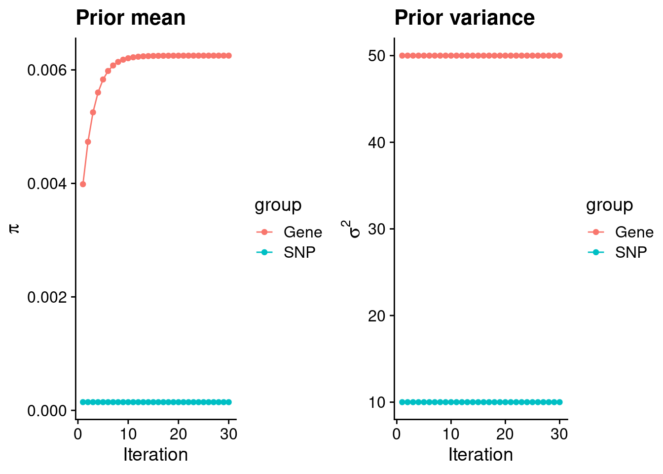
| Version | Author | Date |
|---|---|---|
| b14741c | wesleycrouse | 2021-09-06 |
#estimated group prior
estimated_group_prior <- group_prior_rec[,ncol(group_prior_rec)]
names(estimated_group_prior) <- c("gene", "snp")
estimated_group_prior["snp"] <- estimated_group_prior["snp"]*thin #adjust parameter to account for thin argument
print(estimated_group_prior)
gene snp
0.0062514042 0.0001448313 #estimated group prior variance
estimated_group_prior_var <- group_prior_var_rec[,ncol(group_prior_var_rec)]
names(estimated_group_prior_var) <- c("gene", "snp")
print(estimated_group_prior_var)gene snp
50 10 #report sample size
print(sample_size)[1] 292933#report group size
group_size <- c(nrow(ctwas_gene_res), n_snps)
print(group_size)[1] 10901 8697330#estimated group PVE
estimated_group_pve <- estimated_group_prior_var*estimated_group_prior*group_size/sample_size #check PVE calculation
names(estimated_group_pve) <- c("gene", "snp")
print(estimated_group_pve) gene snp
0.01163177 0.04300114 #compare sum(PIP*mu2/sample_size) with above PVE calculation
c(sum(ctwas_gene_res$PVE),sum(ctwas_snp_res$PVE))[1] 0.01191521 0.48019989Genes with highest PIPs
#distribution of PIPs
hist(ctwas_gene_res$susie_pip, xlim=c(0,1), main="Distribution of Gene PIPs")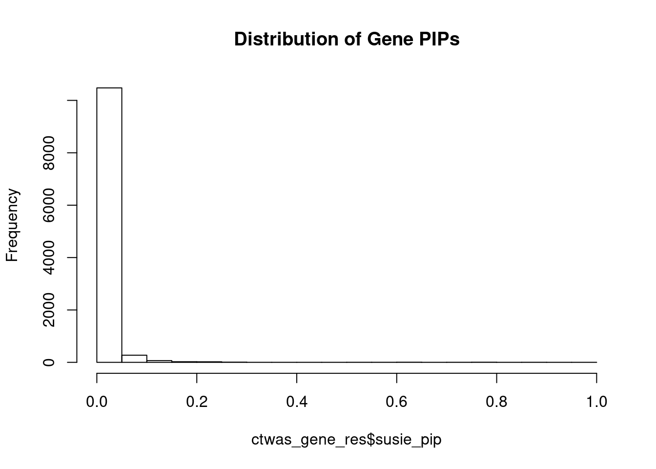
| Version | Author | Date |
|---|---|---|
| b14741c | wesleycrouse | 2021-09-06 |
#genes with PIP>0.8 or 20 highest PIPs
head(ctwas_gene_res[order(-ctwas_gene_res$susie_pip),report_cols], max(sum(ctwas_gene_res$susie_pip>0.8), 20))
genename region_tag susie_pip mu2 PVE z
12467 RP11-219B17.3 15_27 0.988 54.95 1.9e-04 7.18
3212 CCND2 12_4 0.982 32.46 1.1e-04 5.34
7040 INHBB 2_70 0.948 27.18 8.8e-05 4.81
5563 ABCG8 2_27 0.895 38.43 1.2e-04 5.88
1320 CWF19L1 10_64 0.895 33.84 1.0e-04 -7.09
3562 ACVR1C 2_94 0.876 25.90 7.7e-05 4.62
2359 ABCC3 17_29 0.825 23.86 6.7e-05 4.38
11790 CYP2A6 19_28 0.789 25.42 6.8e-05 -4.73
10667 HLA-G 6_24 0.781 287.01 7.7e-04 -6.69
1848 CD276 15_35 0.780 39.99 1.1e-04 6.13
7547 LIPC 15_26 0.758 24.65 6.4e-05 3.99
10212 IL27 16_23 0.758 27.82 7.2e-05 -4.76
537 DGAT2 11_42 0.735 58.00 1.5e-04 -7.51
2004 TGFB1 19_28 0.725 41.46 1.0e-04 5.64
4269 ITGB4 17_42 0.714 24.47 6.0e-05 -4.91
6682 CYB5R1 1_102 0.676 26.01 6.0e-05 -3.95
1231 PABPC4 1_24 0.647 26.02 5.7e-05 4.52
12687 RP4-781K5.7 1_121 0.628 22.98 4.9e-05 -4.17
1120 CETP 16_31 0.625 29.40 6.3e-05 -4.03
10495 PRMT6 1_66 0.606 31.38 6.5e-05 5.14Genes with largest effect sizes
#plot PIP vs effect size
plot(ctwas_gene_res$susie_pip, ctwas_gene_res$mu2, xlab="PIP", ylab="mu^2", main="Gene PIPs vs Effect Size")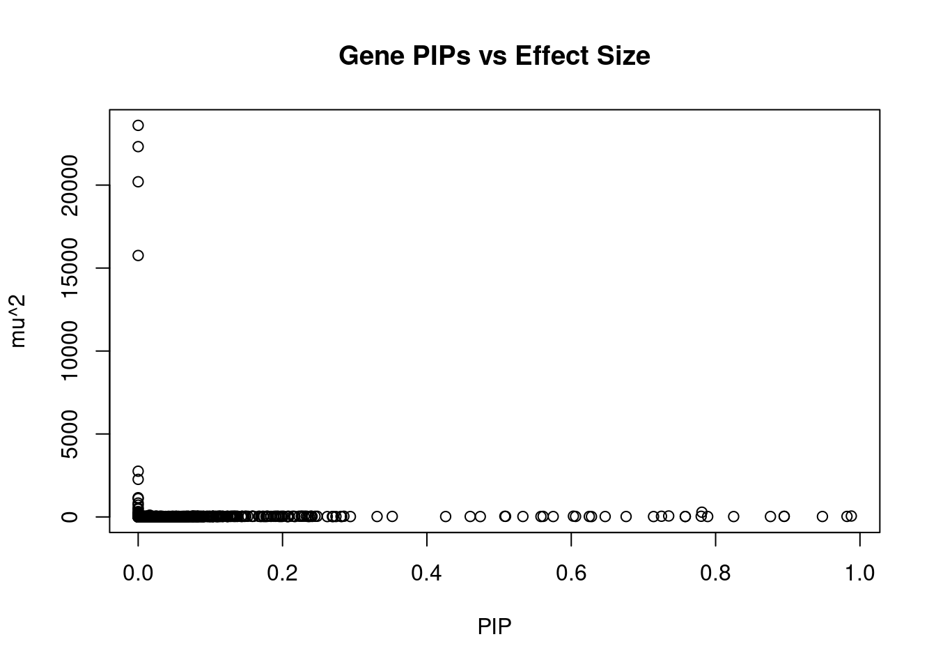
| Version | Author | Date |
|---|---|---|
| b14741c | wesleycrouse | 2021-09-06 |
#genes with 20 largest effect sizes
head(ctwas_gene_res[order(-ctwas_gene_res$mu2),report_cols],20)
genename region_tag susie_pip mu2 PVE z
11533 UGT1A4 2_137 0.000 23599.35 0.0e+00 232.75
11447 UGT1A1 2_137 0.000 22318.31 0.0e+00 -230.41
11489 UGT1A3 2_137 0.000 20201.28 0.0e+00 213.80
7732 UGT1A6 2_137 0.000 15757.53 0.0e+00 186.96
11522 UGT1A7 2_137 0.000 2757.23 0.0e+00 -71.90
12683 HCP5B 6_24 0.000 2265.61 9.9e-09 -3.52
10663 TRIM31 6_24 0.000 1159.83 1.1e-12 1.07
4833 FLOT1 6_24 0.000 1107.05 9.5e-13 -1.07
1088 USP40 2_137 0.000 837.22 0.0e+00 -46.64
10747 SLCO1B7 12_16 0.000 715.07 0.0e+00 12.26
10651 ABCF1 6_24 0.000 534.13 2.7e-10 -3.76
5766 PPP1R18 6_24 0.000 471.56 4.7e-10 -3.94
2584 SLCO1B3 12_16 0.000 324.95 0.0e+00 9.93
10667 HLA-G 6_24 0.781 287.01 7.7e-04 -6.69
4836 NRM 6_24 0.000 251.96 4.7e-14 -0.40
4482 SPX 12_16 0.000 180.88 0.0e+00 4.60
624 ZNRD1 6_24 0.000 178.49 3.8e-14 0.19
36 RECQL 12_16 0.000 148.06 0.0e+00 3.81
3400 IAPP 12_16 0.000 116.63 0.0e+00 5.16
8651 MSL2 3_84 0.016 107.80 5.8e-06 10.28Genes with highest PVE
#genes with 20 highest pve
head(ctwas_gene_res[order(-ctwas_gene_res$PVE),report_cols],20)
genename region_tag susie_pip mu2 PVE z
10667 HLA-G 6_24 0.781 287.01 7.7e-04 -6.69
12467 RP11-219B17.3 15_27 0.988 54.95 1.9e-04 7.18
537 DGAT2 11_42 0.735 58.00 1.5e-04 -7.51
5563 ABCG8 2_27 0.895 38.43 1.2e-04 5.88
3212 CCND2 12_4 0.982 32.46 1.1e-04 5.34
1848 CD276 15_35 0.780 39.99 1.1e-04 6.13
1320 CWF19L1 10_64 0.895 33.84 1.0e-04 -7.09
2004 TGFB1 19_28 0.725 41.46 1.0e-04 5.64
10000 ZKSCAN3 6_22 0.603 46.85 9.6e-05 3.82
7040 INHBB 2_70 0.948 27.18 8.8e-05 4.81
3562 ACVR1C 2_94 0.876 25.90 7.7e-05 4.62
10212 IL27 16_23 0.758 27.82 7.2e-05 -4.76
11669 RP11-452H21.4 11_43 0.508 39.09 6.8e-05 5.78
11790 CYP2A6 19_28 0.789 25.42 6.8e-05 -4.73
2359 ABCC3 17_29 0.825 23.86 6.7e-05 4.38
10495 PRMT6 1_66 0.606 31.38 6.5e-05 5.14
7547 LIPC 15_26 0.758 24.65 6.4e-05 3.99
8142 CNTROB 17_7 0.561 33.40 6.4e-05 -5.71
1120 CETP 16_31 0.625 29.40 6.3e-05 -4.03
2924 EFHD1 2_136 0.509 35.87 6.2e-05 6.05Genes with largest z scores
#genes with 20 largest z scores
head(ctwas_gene_res[order(-abs(ctwas_gene_res$z)),report_cols],20)
genename region_tag susie_pip mu2 PVE z
11533 UGT1A4 2_137 0.000 23599.35 0.0e+00 232.75
11447 UGT1A1 2_137 0.000 22318.31 0.0e+00 -230.41
11489 UGT1A3 2_137 0.000 20201.28 0.0e+00 213.80
7732 UGT1A6 2_137 0.000 15757.53 0.0e+00 186.96
11522 UGT1A7 2_137 0.000 2757.23 0.0e+00 -71.90
1088 USP40 2_137 0.000 837.22 0.0e+00 -46.64
10747 SLCO1B7 12_16 0.000 715.07 0.0e+00 12.26
3556 HJURP 2_137 0.000 101.54 0.0e+00 10.96
8651 MSL2 3_84 0.016 107.80 5.8e-06 10.28
2584 SLCO1B3 12_16 0.000 324.95 0.0e+00 9.93
2586 GOLT1B 12_16 0.000 84.62 0.0e+00 7.53
537 DGAT2 11_42 0.735 58.00 1.5e-04 -7.51
11290 MAPKAPK5-AS1 12_67 0.015 52.80 2.7e-06 -7.21
12467 RP11-219B17.3 15_27 0.988 54.95 1.9e-04 7.18
2541 ALDH2 12_67 0.012 49.97 2.0e-06 7.10
1320 CWF19L1 10_64 0.895 33.84 1.0e-04 -7.09
2536 SH2B3 12_67 0.004 41.59 5.5e-07 6.80
10667 HLA-G 6_24 0.781 287.01 7.7e-04 -6.69
2170 AHR 7_17 0.007 48.66 1.1e-06 -6.58
4962 EXOC6 10_59 0.012 57.26 2.3e-06 -6.37Comparing z scores and PIPs
#set nominal signifiance threshold for z scores
alpha <- 0.05

#bonferroni adjusted threshold for z scores
sig_thresh <- qnorm(1-(alpha/nrow(ctwas_gene_res)/2), lower=T)

#Q-Q plot for z scores
obs_z <- ctwas_gene_res$z[order(ctwas_gene_res$z)]
exp_z <- qnorm((1:nrow(ctwas_gene_res))/nrow(ctwas_gene_res))

plot(exp_z, obs_z, xlab="Expected z", ylab="Observed z", main="Gene z score Q-Q plot")
abline(a=0,b=1)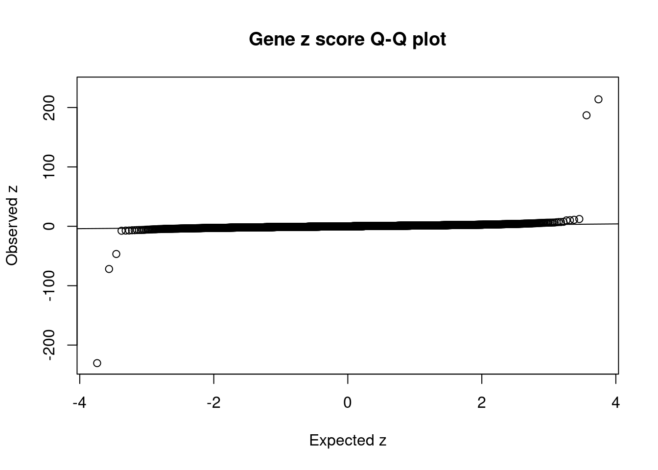
| Version | Author | Date |
|---|---|---|
| b14741c | wesleycrouse | 2021-09-06 |
#plot z score vs PIP
plot(abs(ctwas_gene_res$z), ctwas_gene_res$susie_pip, xlab="abs(z)", ylab="PIP")
abline(v=sig_thresh, col="red", lty=2)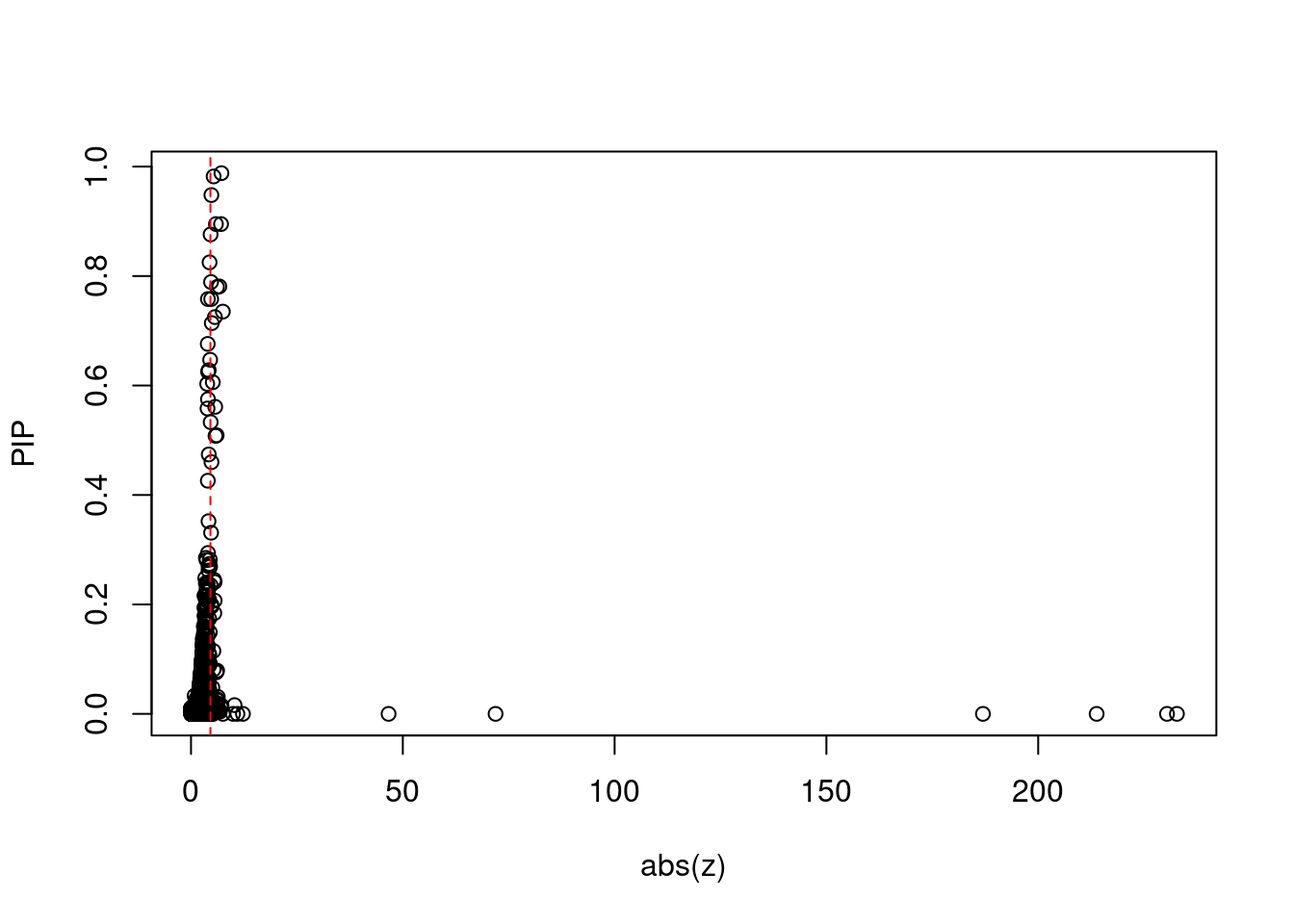
| Version | Author | Date |
|---|---|---|
| b14741c | wesleycrouse | 2021-09-06 |
#proportion of significant z scores
mean(abs(ctwas_gene_res$z) > sig_thresh)
[1] 0.006696633#genes with most significant z scores
head(ctwas_gene_res[order(-abs(ctwas_gene_res$z)),report_cols],20) genename region_tag susie_pip mu2 PVE z
11533 UGT1A4 2_137 0.000 23599.35 0.0e+00 232.75
11447 UGT1A1 2_137 0.000 22318.31 0.0e+00 -230.41
11489 UGT1A3 2_137 0.000 20201.28 0.0e+00 213.80
7732 UGT1A6 2_137 0.000 15757.53 0.0e+00 186.96
11522 UGT1A7 2_137 0.000 2757.23 0.0e+00 -71.90
1088 USP40 2_137 0.000 837.22 0.0e+00 -46.64
10747 SLCO1B7 12_16 0.000 715.07 0.0e+00 12.26
3556 HJURP 2_137 0.000 101.54 0.0e+00 10.96
8651 MSL2 3_84 0.016 107.80 5.8e-06 10.28
2584 SLCO1B3 12_16 0.000 324.95 0.0e+00 9.93
2586 GOLT1B 12_16 0.000 84.62 0.0e+00 7.53
537 DGAT2 11_42 0.735 58.00 1.5e-04 -7.51
11290 MAPKAPK5-AS1 12_67 0.015 52.80 2.7e-06 -7.21
12467 RP11-219B17.3 15_27 0.988 54.95 1.9e-04 7.18
2541 ALDH2 12_67 0.012 49.97 2.0e-06 7.10
1320 CWF19L1 10_64 0.895 33.84 1.0e-04 -7.09
2536 SH2B3 12_67 0.004 41.59 5.5e-07 6.80
10667 HLA-G 6_24 0.781 287.01 7.7e-04 -6.69
2170 AHR 7_17 0.007 48.66 1.1e-06 -6.58
4962 EXOC6 10_59 0.012 57.26 2.3e-06 -6.37Locus plots for genes and SNPs
ctwas_gene_res_sortz <- ctwas_gene_res[order(-abs(ctwas_gene_res$z)),]

n_plots <- 5
for (region_tag_plot in head(unique(ctwas_gene_res_sortz$region_tag), n_plots)){
  ctwas_res_region <-  ctwas_res[ctwas_res$region_tag==region_tag_plot,]
  start <- min(ctwas_res_region$pos)
  end <- max(ctwas_res_region$pos)

  ctwas_res_region <- ctwas_res_region[order(ctwas_res_region$pos),]
  ctwas_res_region_gene <- ctwas_res_region[ctwas_res_region$type=="gene",]
  ctwas_res_region_snp <- ctwas_res_region[ctwas_res_region$type=="SNP",]

  #region name
  print(paste0("Region: ", region_tag_plot))

  #table of genes in region
  print(ctwas_res_region_gene[,report_cols])

  par(mfrow=c(4,1))

  #gene z scores
  plot(ctwas_res_region_gene$pos, abs(ctwas_res_region_gene$z), xlab="Position", ylab="abs(gene_z)", xlim=c(start,end),
   ylim=c(0,max(sig_thresh, abs(ctwas_res_region_gene$z))),
   main=paste0("Region: ", region_tag_plot))
  abline(h=sig_thresh,col="red",lty=2)

  #significance threshold for SNPs
  alpha_snp <- 5*10^(-8)
  sig_thresh_snp <- qnorm(1-alpha_snp/2, lower=T)

  #snp z scores
  plot(ctwas_res_region_snp$pos, abs(ctwas_res_region_snp$z), xlab="Position", ylab="abs(snp_z)",xlim=c(start,end),
   ylim=c(0,max(sig_thresh_snp, max(abs(ctwas_res_region_snp$z)))))
  abline(h=sig_thresh_snp,col="purple",lty=2)

  #gene pips
  plot(ctwas_res_region_gene$pos, ctwas_res_region_gene$susie_pip, xlab="Position", ylab="Gene PIP", xlim=c(start,end), ylim=c(0,1))
  abline(h=0.8,col="blue",lty=2)

  #snp pips
  plot(ctwas_res_region_snp$pos, ctwas_res_region_snp$susie_pip, xlab="Position", ylab="SNP PIP", xlim=c(start,end), ylim=c(0,1))
  abline(h=0.8,col="blue",lty=2)
}
[1] "Region: 2_137"
genename region_tag susie_pip mu2 PVE z
10567 GIGYF2 2_137 0 17.81 0 -5.12
9340 C2orf82 2_137 0 8.33 0 0.45
620 NGEF 2_137 0 9.62 0 2.52
8006 INPP5D 2_137 0 16.92 0 4.05
879 DGKD 2_137 0 43.46 0 -0.07
1088 USP40 2_137 0 837.22 0 -46.64
11522 UGT1A7 2_137 0 2757.23 0 -71.90
7732 UGT1A6 2_137 0 15757.53 0 186.96
11533 UGT1A4 2_137 0 23599.35 0 232.75
11489 UGT1A3 2_137 0 20201.28 0 213.80
11447 UGT1A1 2_137 0 22318.31 0 -230.41
3556 HJURP 2_137 0 101.54 0 10.96
11098 AC006037.2 2_137 0 5.32 0 1.50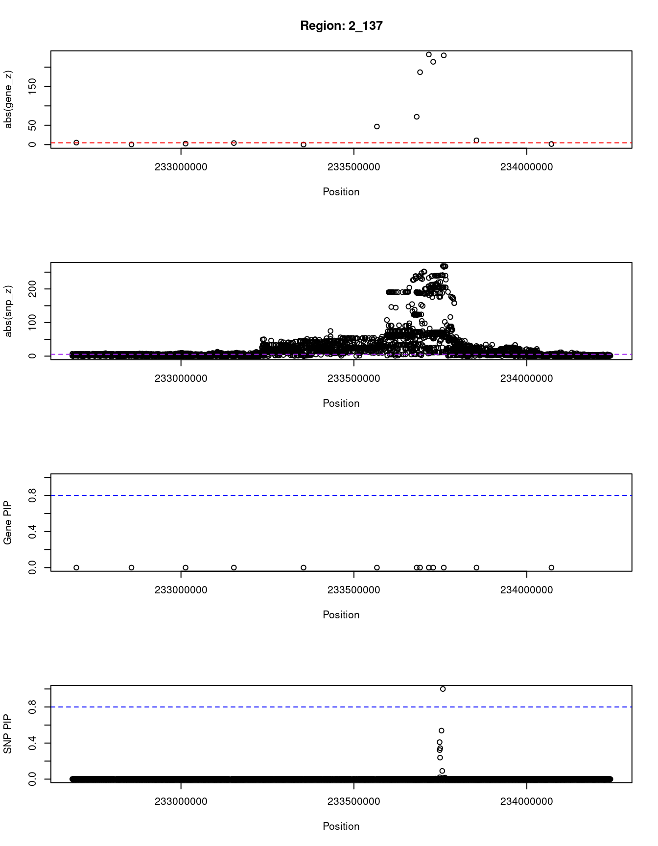
| Version | Author | Date |
|---|---|---|
| b14741c | wesleycrouse | 2021-09-06 |
[1] "Region: 12_16"
      genename region_tag susie_pip    mu2 PVE     z
2584   SLCO1B3      12_16         0 324.95   0  9.93
10747  SLCO1B7      12_16         0 715.07   0 12.26
3400      IAPP      12_16         0 116.63   0  5.16
3399   PYROXD1      12_16         0  13.15   0  0.89
36       RECQL      12_16         0 148.06   0  3.81
2586    GOLT1B      12_16         0  84.62   0  7.53
4482       SPX      12_16         0 180.88   0  4.60
2587      LDHB      12_16         0   9.74   0  0.07
3401     KCNJ8      12_16         0   6.99   0 -0.33
689      ABCC9      12_16         0   7.75   0  2.11
2590     C2CD5      12_16         0  12.90   0 -1.39
5073     ETNK1      12_16         0  10.39   0  0.30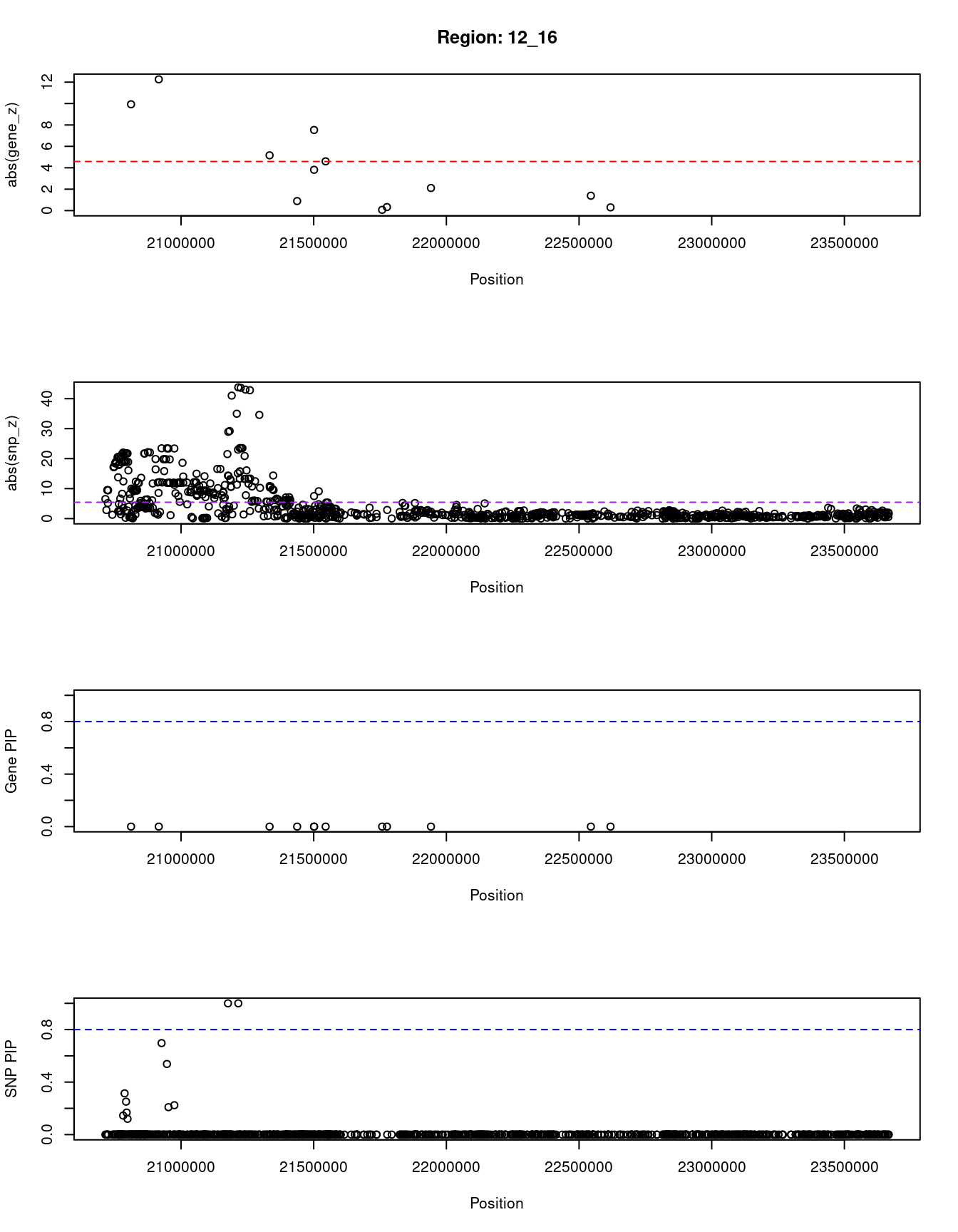
| Version | Author | Date |
|---|---|---|
| b14741c | wesleycrouse | 2021-09-06 |
[1] "Region: 3_84"
     genename region_tag susie_pip    mu2     PVE     z
796   PPP2R3A       3_84     0.015  17.35 9.0e-07 -2.46
8651     MSL2       3_84     0.016 107.80 5.8e-06 10.28
2795     PCCB       3_84     0.006   6.41 1.2e-07  1.22
3148    STAG1       3_84     0.006   5.50 1.1e-07 -0.03
6584     NCK1       3_84     0.006   9.53 1.8e-07 -2.19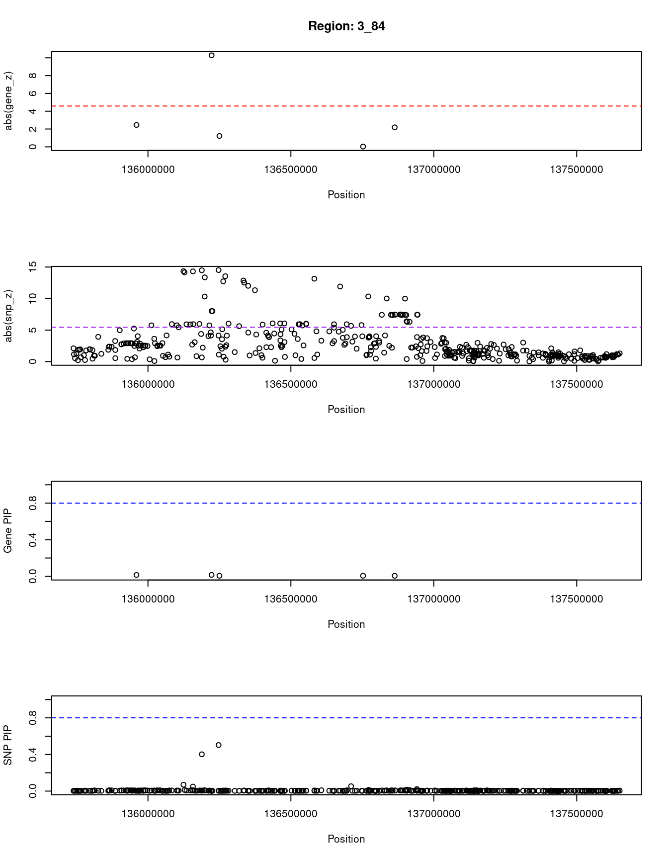
| Version | Author | Date |
|---|---|---|
| b14741c | wesleycrouse | 2021-09-06 |
[1] "Region: 11_42"
           genename region_tag susie_pip   mu2     PVE     z
7611          XRRA1      11_42     0.009  9.35 2.7e-07 -1.00
3170          SPCS2      11_42     0.006  6.60 1.4e-07  0.73
6901           NEU3      11_42     0.005  5.10 9.5e-08  0.39
4848        SLCO2B1      11_42     0.006  5.13 9.6e-08 -0.22
12001         TPBGL      11_42     0.008  8.50 2.3e-07  0.68
6617          GDPD5      11_42     0.008 11.91 3.3e-07  1.95
8328           MAP6      11_42     0.007  7.49 1.9e-07  0.24
7603         MOGAT2      11_42     0.033 19.53 2.2e-06  0.85
537           DGAT2      11_42     0.735 58.00 1.5e-04 -7.51
10381         UVRAG      11_42     0.006  7.49 1.6e-07  1.62
1082          WNT11      11_42     0.008  9.14 2.5e-07  1.06
11773 RP11-619A14.3      11_42     0.006  6.63 1.4e-07  0.61
4849         THAP12      11_42     0.006  6.04 1.2e-07 -0.66
12265 RP11-111M22.5      11_42     0.007  7.23 1.7e-07  0.80
11766 RP11-111M22.3      11_42     0.005  5.17 9.7e-08  0.31
11751  RP11-672A2.4      11_42     0.006  6.00 1.2e-07  0.53
9350           TSKU      11_42     0.006  5.62 1.1e-07  0.25
905           ACER3      11_42     0.025 19.70 1.7e-06 -2.04
5976          CAPN5      11_42     0.017 16.17 9.2e-07  1.72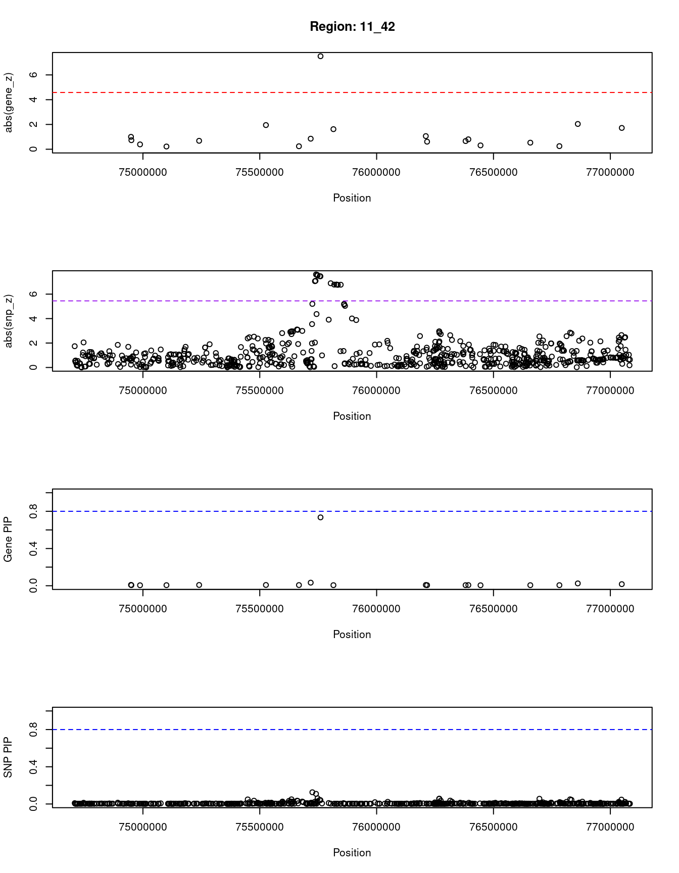
| Version | Author | Date |
|---|---|---|
| b14741c | wesleycrouse | 2021-09-06 |
[1] "Region: 12_67"
          genename region_tag susie_pip   mu2     PVE     z
5112          TCHP      12_67     0.087 18.95 5.6e-06  3.21
5111          GIT2      12_67     0.053 18.09 3.3e-06  3.36
8639      C12orf76      12_67     0.004  7.15 1.0e-07 -0.30
3515         IFT81      12_67     0.005 13.07 2.3e-07  2.50
10093       ANAPC7      12_67     0.005 11.10 2.0e-07  2.16
2531         ARPC3      12_67     0.005  8.92 1.6e-07  0.54
10684      FAM216A      12_67     0.004 11.28 1.6e-07  2.42
2532          GPN3      12_67     0.003  6.71 7.9e-08  1.40
2533         VPS29      12_67     0.003  6.80 8.1e-08 -1.41
10683        TCTN1      12_67     0.004  7.01 1.0e-07  0.02
3517         HVCN1      12_67     0.009 17.42 5.6e-07  2.67
9717        PPP1CC      12_67     0.009 17.33 5.5e-07 -2.65
10375      FAM109A      12_67     0.004  8.59 1.0e-07 -1.46
2536         SH2B3      12_67     0.004 41.59 5.5e-07  6.80
10680        ATXN2      12_67     0.004 22.35 2.8e-07  3.97
2541         ALDH2      12_67     0.012 49.97 2.0e-06  7.10
11290 MAPKAPK5-AS1      12_67     0.015 52.80 2.7e-06 -7.21
1191         ERP29      12_67     0.025 44.67 3.9e-06  6.25
10370      TMEM116      12_67     0.025 44.67 3.9e-06 -6.25
2544         NAA25      12_67     0.020 41.48 2.8e-06 -6.12
8505        HECTD4      12_67     0.031 48.79 5.1e-06  6.33
9084        PTPN11      12_67     0.004  7.73 1.1e-07 -0.78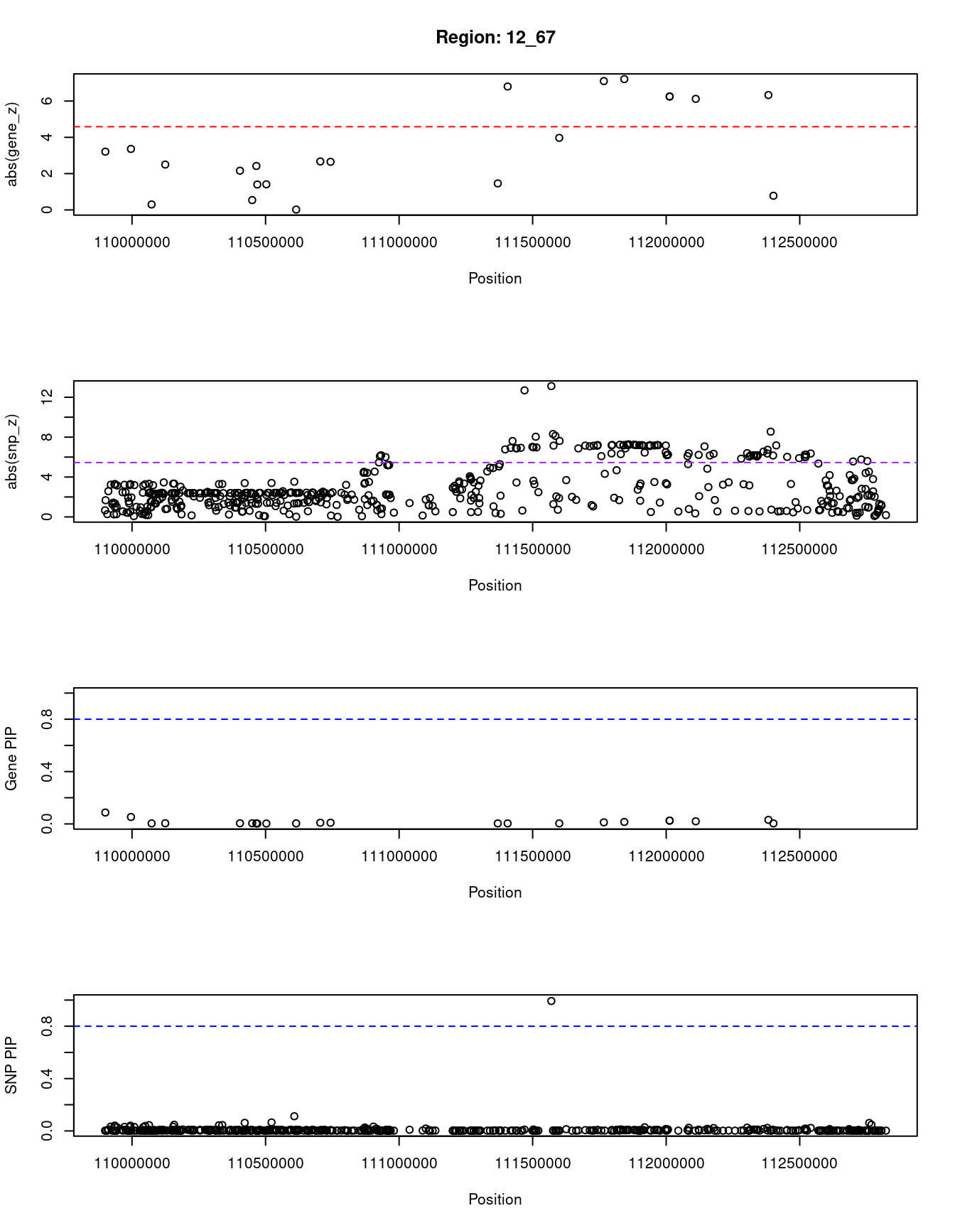
| Version | Author | Date |
|---|---|---|
| b14741c | wesleycrouse | 2021-09-06 |
SNPs with highest PIPs
#snps with PIP>0.8 or 20 highest PIPs
head(ctwas_snp_res[order(-ctwas_snp_res$susie_pip),report_cols_snps],
max(sum(ctwas_snp_res$susie_pip>0.8), 20))
id region_tag susie_pip mu2 PVE z
328040 rs72834643 6_20 1.000 106.48 3.6e-04 9.73
328061 rs115740542 6_20 1.000 160.00 5.5e-04 12.66
372492 rs12208357 6_103 1.000 68.76 2.3e-04 -6.65
384278 rs542176135 7_17 1.000 123.44 4.2e-04 -8.38
536243 rs6480402 10_46 1.000 226.82 7.7e-04 8.90
606967 rs11045819 12_16 1.000 1856.07 6.3e-03 -14.34
606984 rs4363657 12_16 1.000 1486.76 5.1e-03 43.78
805825 rs59616136 19_14 1.000 44.78 1.5e-04 7.00
813971 rs113345881 19_32 1.000 36.54 1.2e-04 6.12
890179 rs13031505 2_136 1.000 53.91 1.8e-04 -8.07
893719 rs1976391 2_137 1.000 27927.25 9.5e-02 268.40
895635 rs1611236 6_24 1.000 4012.69 1.4e-02 -3.60
329231 rs3130253 6_23 0.999 36.87 1.3e-04 -6.63
557539 rs76153913 11_2 0.999 52.65 1.8e-04 6.70
511528 rs115478735 9_70 0.998 57.97 2.0e-04 -8.02
813969 rs814573 19_32 0.998 34.01 1.2e-04 -6.68
536242 rs4745982 10_46 0.995 58.34 2.0e-04 11.95
890116 rs34247311 2_136 0.995 34.59 1.2e-04 4.44
617657 rs7397189 12_36 0.994 31.94 1.1e-04 5.69
825702 rs34507316 20_13 0.994 28.59 9.7e-05 5.60
634243 rs653178 12_67 0.993 144.66 4.9e-04 -13.12
804054 rs141645070 19_10 0.991 27.74 9.4e-05 -5.27
557544 rs2519158 11_2 0.983 33.90 1.1e-04 5.74
813974 rs12721109 19_32 0.977 29.67 9.9e-05 6.44
384300 rs4721597 7_17 0.976 64.38 2.1e-04 1.94
36885 rs2779116 1_78 0.971 63.50 2.1e-04 -8.25
557537 rs10832897 11_2 0.964 29.80 9.8e-05 -2.62
751839 rs2608604 16_53 0.963 50.17 1.6e-04 -6.33
713221 rs2070895 15_26 0.953 29.70 9.7e-05 -5.24
813905 rs1551891 19_32 0.944 33.76 1.1e-04 7.88
806610 rs3794991 19_15 0.943 118.76 3.8e-04 11.64
234941 rs17238095 4_72 0.931 27.62 8.8e-05 5.18
606687 rs73080739 12_15 0.930 31.63 1.0e-04 -7.24
854778 rs34662558 22_10 0.924 27.91 8.8e-05 -5.19
511913 rs34755157 9_71 0.919 26.56 8.3e-05 -5.03
561992 rs34623292 11_10 0.917 27.27 8.5e-05 -5.06
606682 rs7962574 12_15 0.916 43.97 1.4e-04 -8.40
497446 rs9410381 9_45 0.893 68.36 2.1e-04 8.62
439954 rs12549737 8_24 0.890 27.33 8.3e-05 5.15
817150 rs71185869 19_36 0.882 24.36 7.3e-05 4.56
296256 rs4566840 5_66 0.839 29.07 8.3e-05 -5.46
277741 rs79086423 5_29 0.836 24.25 6.9e-05 4.53
670004 rs35115456 13_53 0.834 24.97 7.1e-05 -4.47
760017 rs62640050 17_17 0.832 24.30 6.9e-05 -4.59
65060 rs12239046 1_131 0.829 25.06 7.1e-05 -4.57
606722 rs10770693 12_15 0.829 55.90 1.6e-04 8.86
560561 rs4910498 11_8 0.827 48.19 1.4e-04 6.71
857529 rs6000553 22_14 0.827 39.94 1.1e-04 6.47
749728 rs11641197 16_49 0.819 25.05 7.0e-05 -4.43
34678 rs12124727 1_73 0.816 25.34 7.1e-05 -4.54
255620 rs12651414 4_113 0.802 26.00 7.1e-05 4.71
506145 rs10759697 9_59 0.802 27.81 7.6e-05 -5.05SNPs with largest effect sizes
#plot PIP vs effect size
plot(ctwas_snp_res$susie_pip, ctwas_snp_res$mu2, xlab="PIP", ylab="mu^2", main="SNP PIPs vs Effect Size")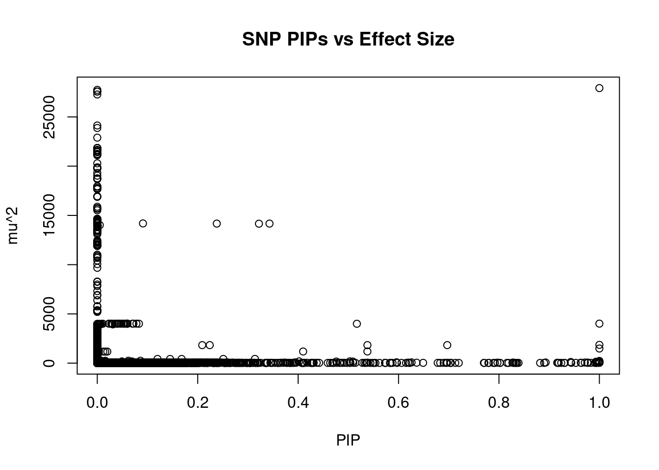
| Version | Author | Date |
|---|---|---|
| b14741c | wesleycrouse | 2021-09-06 |
#SNPs with 50 largest effect sizes
head(ctwas_snp_res[order(-ctwas_snp_res$mu2),report_cols_snps],50)
id region_tag susie_pip mu2 PVE z
893719 rs1976391 2_137 1 27927.25 9.5e-02 268.40
893728 rs887829 2_137 0 27748.16 8.9e-16 267.84
893737 rs4148325 2_137 0 27577.86 0.0e+00 267.14
893733 rs6742078 2_137 0 27576.43 0.0e+00 267.16
893735 rs4148324 2_137 0 27573.07 0.0e+00 267.15
893729 rs34983651 2_137 0 27275.91 0.0e+00 265.62
893480 rs17863787 2_137 0 24129.83 0.0e+00 252.20
893482 rs7567229 2_137 0 23874.95 0.0e+00 251.23
893465 rs28899170 2_137 0 22896.22 0.0e+00 247.07
893712 rs6714634 2_137 0 21849.64 0.0e+00 240.76
893718 rs10929302 2_137 0 21841.51 0.0e+00 240.75
893698 rs2885296 2_137 0 21840.50 0.0e+00 240.61
893709 rs6747843 2_137 0 21837.35 0.0e+00 240.71
893628 rs7567468 2_137 0 21645.52 0.0e+00 239.52
893670 rs17864701 2_137 0 21628.96 0.0e+00 239.62
893679 rs11695484 2_137 0 21627.98 0.0e+00 239.66
893656 rs34352510 2_137 0 21624.98 0.0e+00 239.54
893651 rs17862875 2_137 0 21623.10 0.0e+00 239.53
893736 rs3771341 2_137 0 21616.55 0.0e+00 239.79
893643 rs6722076 2_137 0 21493.41 0.0e+00 238.91
893587 rs112132688 2_137 0 21420.56 0.0e+00 238.55
893383 rs11692664 2_137 0 21240.53 0.0e+00 238.08
893377 rs7571915 2_137 0 21230.78 0.0e+00 238.05
893457 rs2070959 2_137 0 21223.97 0.0e+00 238.14
893436 rs10173355 2_137 0 21211.16 0.0e+00 238.10
893435 rs10168416 2_137 0 21211.15 0.0e+00 238.10
893585 rs202203863 2_137 0 21199.15 0.0e+00 237.52
893386 rs10202865 2_137 0 21110.10 0.0e+00 237.49
893539 rs6744284 2_137 0 20291.87 0.0e+00 232.75
893456 rs1105880 2_137 0 19883.77 0.0e+00 232.16
893458 rs1105879 2_137 0 19844.61 0.0e+00 231.91
893391 rs35984508 2_137 0 19812.85 0.0e+00 231.56
893390 rs75444879 2_137 0 19784.52 0.0e+00 231.44
893389 rs77070100 2_137 0 19765.89 0.0e+00 231.38
893470 rs6715829 2_137 0 19317.56 0.0e+00 229.45
893745 rs929596 2_137 0 19037.92 0.0e+00 227.71
893360 rs2602376 2_137 0 18760.44 0.0e+00 227.08
893350 rs2741046 2_137 0 18753.27 0.0e+00 227.06
893349 rs2741045 2_137 0 18716.79 0.0e+00 226.92
893344 rs2741044 2_137 0 18686.69 0.0e+00 226.76
893630 rs7576166 2_137 0 17952.36 0.0e+00 213.95
893650 rs2018985 2_137 0 17946.94 0.0e+00 213.92
893632 rs4477910 2_137 0 17924.80 0.0e+00 213.81
893697 rs12987866 2_137 0 17782.48 0.0e+00 220.81
893611 rs6431625 2_137 0 17765.43 0.0e+00 212.64
893603 rs1983023 2_137 0 17760.45 0.0e+00 212.90
893583 rs6750992 2_137 0 17687.89 0.0e+00 212.83
893667 rs13009407 2_137 0 17662.19 0.0e+00 220.02
893531 rs6749496 2_137 0 16941.36 0.0e+00 208.13
893642 rs17862873 2_137 0 16921.52 0.0e+00 215.62SNPs with highest PVE
#SNPs with 50 highest pve
head(ctwas_snp_res[order(-ctwas_snp_res$PVE),report_cols_snps],50)
id region_tag susie_pip mu2 PVE z
893719 rs1976391 2_137 1.000 27927.25 0.09500 268.40
893693 rs7604115 2_137 0.343 14168.33 0.01700 187.81
893686 rs11888459 2_137 0.322 14158.90 0.01600 187.72
895635 rs1611236 6_24 1.000 4012.69 0.01400 -3.60
893690 rs10178992 2_137 0.238 14170.56 0.01200 187.81
895647 rs1611241 6_24 0.517 3999.61 0.00710 -3.84
606967 rs11045819 12_16 1.000 1856.07 0.00630 -14.34
606984 rs4363657 12_16 1.000 1486.76 0.00510 43.78
606868 rs12366506 12_16 0.697 1832.47 0.00440 23.44
893707 rs11673726 2_137 0.091 14187.10 0.00440 187.95
606874 rs11045612 12_16 0.538 1830.88 0.00340 23.44
893704 rs17862878 2_137 0.538 1185.09 0.00220 -11.26
893685 rs12466997 2_137 0.410 1183.03 0.00170 -11.17
606885 rs73062442 12_16 0.224 1830.04 0.00140 23.39
606877 rs11513221 12_16 0.209 1829.98 0.00130 23.38
895553 rs1633033 6_24 0.078 4011.80 0.00110 -3.63
895701 rs9258382 6_24 0.083 4002.92 0.00110 -3.69
895658 rs1611248 6_24 0.072 4011.84 0.00099 -3.63
895916 rs1633001 6_24 0.070 4010.11 0.00096 -3.64
895566 rs2844838 6_24 0.060 4011.54 0.00082 -3.63
895614 rs2508055 6_24 0.060 4011.62 0.00082 -3.62
895617 rs111734624 6_24 0.060 4011.62 0.00082 -3.62
895662 rs1611252 6_24 0.059 4011.63 0.00081 -3.62
895679 rs1611260 6_24 0.059 4011.62 0.00081 -3.62
895685 rs1611265 6_24 0.059 4011.62 0.00081 -3.62
536243 rs6480402 10_46 1.000 226.82 0.00077 8.90
895888 rs3129185 6_24 0.056 4010.33 0.00076 -3.63
896092 rs1632980 6_24 0.054 4009.68 0.00074 -3.63
895589 rs1614309 6_24 0.053 4008.66 0.00072 -3.63
895903 rs1736999 6_24 0.051 4010.11 0.00069 -3.63
895570 rs1633032 6_24 0.048 4011.14 0.00066 -3.62
895561 rs2844840 6_24 0.047 4010.17 0.00064 -3.62
895621 rs1611228 6_24 0.044 4011.33 0.00060 -3.62
895687 rs1611267 6_24 0.043 4011.31 0.00059 -3.62
328061 rs115740542 6_20 1.000 160.00 0.00055 12.66
895689 rs2394171 6_24 0.040 4011.26 0.00055 -3.61
895691 rs2893981 6_24 0.040 4011.25 0.00055 -3.61
895656 rs1611246 6_24 0.038 4009.43 0.00052 -3.62
634243 rs653178 12_67 0.993 144.66 0.00049 -13.12
895604 rs1633020 6_24 0.035 4010.68 0.00047 -3.61
606778 rs3060461 12_16 0.314 429.45 0.00046 -21.86
384278 rs542176135 7_17 1.000 123.44 0.00042 -8.38
895493 rs1610726 6_24 0.030 4010.14 0.00041 -3.61
895659 rs1611249 6_24 0.031 3936.54 0.00041 -4.10
806610 rs3794991 19_15 0.943 118.76 0.00038 11.64
895610 rs1737020 6_24 0.028 4010.90 0.00038 -3.60
895611 rs1737019 6_24 0.028 4010.90 0.00038 -3.60
606782 rs35290079 12_16 0.251 427.23 0.00037 -21.76
328040 rs72834643 6_20 1.000 106.48 0.00036 9.73
895633 rs1611234 6_24 0.024 4010.18 0.00033 -3.60SNPs with largest z scores
#SNPs with 50 largest z scores
head(ctwas_snp_res[order(-abs(ctwas_snp_res$z)),report_cols_snps],50)
id region_tag susie_pip mu2 PVE z
893719 rs1976391 2_137 1 27927.25 9.5e-02 268.40
893728 rs887829 2_137 0 27748.16 8.9e-16 267.84
893733 rs6742078 2_137 0 27576.43 0.0e+00 267.16
893735 rs4148324 2_137 0 27573.07 0.0e+00 267.15
893737 rs4148325 2_137 0 27577.86 0.0e+00 267.14
893729 rs34983651 2_137 0 27275.91 0.0e+00 265.62
893480 rs17863787 2_137 0 24129.83 0.0e+00 252.20
893482 rs7567229 2_137 0 23874.95 0.0e+00 251.23
893465 rs28899170 2_137 0 22896.22 0.0e+00 247.07
893712 rs6714634 2_137 0 21849.64 0.0e+00 240.76
893718 rs10929302 2_137 0 21841.51 0.0e+00 240.75
893709 rs6747843 2_137 0 21837.35 0.0e+00 240.71
893698 rs2885296 2_137 0 21840.50 0.0e+00 240.61
893736 rs3771341 2_137 0 21616.55 0.0e+00 239.79
893679 rs11695484 2_137 0 21627.98 0.0e+00 239.66
893670 rs17864701 2_137 0 21628.96 0.0e+00 239.62
893656 rs34352510 2_137 0 21624.98 0.0e+00 239.54
893651 rs17862875 2_137 0 21623.10 0.0e+00 239.53
893628 rs7567468 2_137 0 21645.52 0.0e+00 239.52
893643 rs6722076 2_137 0 21493.41 0.0e+00 238.91
893587 rs112132688 2_137 0 21420.56 0.0e+00 238.55
893457 rs2070959 2_137 0 21223.97 0.0e+00 238.14
893435 rs10168416 2_137 0 21211.15 0.0e+00 238.10
893436 rs10173355 2_137 0 21211.16 0.0e+00 238.10
893383 rs11692664 2_137 0 21240.53 0.0e+00 238.08
893377 rs7571915 2_137 0 21230.78 0.0e+00 238.05
893585 rs202203863 2_137 0 21199.15 0.0e+00 237.52
893386 rs10202865 2_137 0 21110.10 0.0e+00 237.49
893539 rs6744284 2_137 0 20291.87 0.0e+00 232.75
893456 rs1105880 2_137 0 19883.77 0.0e+00 232.16
893458 rs1105879 2_137 0 19844.61 0.0e+00 231.91
893391 rs35984508 2_137 0 19812.85 0.0e+00 231.56
893390 rs75444879 2_137 0 19784.52 0.0e+00 231.44
893389 rs77070100 2_137 0 19765.89 0.0e+00 231.38
893470 rs6715829 2_137 0 19317.56 0.0e+00 229.45
893745 rs929596 2_137 0 19037.92 0.0e+00 227.71
893360 rs2602376 2_137 0 18760.44 0.0e+00 227.08
893350 rs2741046 2_137 0 18753.27 0.0e+00 227.06
893349 rs2741045 2_137 0 18716.79 0.0e+00 226.92
893344 rs2741044 2_137 0 18686.69 0.0e+00 226.76
893697 rs12987866 2_137 0 17782.48 0.0e+00 220.81
893667 rs13009407 2_137 0 17662.19 0.0e+00 220.02
893642 rs17862873 2_137 0 16921.52 0.0e+00 215.62
893630 rs7576166 2_137 0 17952.36 0.0e+00 213.95
893650 rs2018985 2_137 0 17946.94 0.0e+00 213.92
893632 rs4477910 2_137 0 17924.80 0.0e+00 213.81
893603 rs1983023 2_137 0 17760.45 0.0e+00 212.90
893583 rs6750992 2_137 0 17687.89 0.0e+00 212.83
893611 rs6431625 2_137 0 17765.43 0.0e+00 212.64
893531 rs6749496 2_137 0 16941.36 0.0e+00 208.13
sessionInfo()R version 3.6.1 (2019-07-05)
Platform: x86_64-pc-linux-gnu (64-bit)
Running under: Scientific Linux 7.4 (Nitrogen)
Matrix products: default
BLAS/LAPACK: /software/openblas-0.2.19-el7-x86_64/lib/libopenblas_haswellp-r0.2.19.so
locale:
[1] LC_CTYPE=en_US.UTF-8 LC_NUMERIC=C
[3] LC_TIME=en_US.UTF-8 LC_COLLATE=en_US.UTF-8
[5] LC_MONETARY=en_US.UTF-8 LC_MESSAGES=en_US.UTF-8
[7] LC_PAPER=en_US.UTF-8 LC_NAME=C
[9] LC_ADDRESS=C LC_TELEPHONE=C
[11] LC_MEASUREMENT=en_US.UTF-8 LC_IDENTIFICATION=C
attached base packages:
[1] stats graphics grDevices utils datasets methods base
other attached packages:
[1] cowplot_1.0.0 ggplot2_3.3.3
loaded via a namespace (and not attached):
[1] Biobase_2.44.0 httr_1.4.1
[3] bit64_4.0.5 assertthat_0.2.1
[5] stats4_3.6.1 blob_1.2.1
[7] BSgenome_1.52.0 GenomeInfoDbData_1.2.1
[9] Rsamtools_2.0.0 yaml_2.2.0
[11] progress_1.2.2 pillar_1.6.1
[13] RSQLite_2.2.7 lattice_0.20-38
[15] glue_1.4.2 digest_0.6.20
[17] GenomicRanges_1.36.0 promises_1.0.1
[19] XVector_0.24.0 colorspace_1.4-1
[21] htmltools_0.3.6 httpuv_1.5.1
[23] Matrix_1.2-18 XML_3.98-1.20
[25] pkgconfig_2.0.3 biomaRt_2.40.1
[27] zlibbioc_1.30.0 purrr_0.3.4
[29] scales_1.1.0 whisker_0.3-2
[31] later_0.8.0 BiocParallel_1.18.0
[33] git2r_0.26.1 tibble_3.1.2
[35] farver_2.1.0 generics_0.0.2
[37] IRanges_2.18.1 ellipsis_0.3.2
[39] withr_2.4.1 cachem_1.0.5
[41] SummarizedExperiment_1.14.1 GenomicFeatures_1.36.3
[43] BiocGenerics_0.30.0 magrittr_2.0.1
[45] crayon_1.4.1 memoise_2.0.0
[47] evaluate_0.14 fs_1.3.1
[49] fansi_0.5.0 tools_3.6.1
[51] data.table_1.14.0 prettyunits_1.0.2
[53] hms_1.1.0 lifecycle_1.0.0
[55] matrixStats_0.57.0 stringr_1.4.0
[57] S4Vectors_0.22.1 munsell_0.5.0
[59] DelayedArray_0.10.0 AnnotationDbi_1.46.0
[61] Biostrings_2.52.0 compiler_3.6.1
[63] GenomeInfoDb_1.20.0 rlang_0.4.11
[65] grid_3.6.1 RCurl_1.98-1.1
[67] VariantAnnotation_1.30.1 labeling_0.3
[69] bitops_1.0-6 rmarkdown_1.13
[71] gtable_0.3.0 DBI_1.1.1
[73] R6_2.5.0 GenomicAlignments_1.20.1
[75] dplyr_1.0.7 knitr_1.23
[77] rtracklayer_1.44.0 utf8_1.2.1
[79] fastmap_1.1.0 bit_4.0.4
[81] workflowr_1.6.2 rprojroot_2.0.2
[83] stringi_1.4.3 parallel_3.6.1
[85] Rcpp_1.0.6 vctrs_0.3.8
[87] tidyselect_1.1.0 xfun_0.8