Direct bilirubin (quantile) - Liver [fixed prior variance]
wesleycrouse
2021-08-18
Last updated: 2021-09-09
Checks: 7 0
Knit directory: ctwas_applied/
This reproducible R Markdown analysis was created with workflowr (version 1.6.2). The Checks tab describes the reproducibility checks that were applied when the results were created. The Past versions tab lists the development history.
Great! Since the R Markdown file has been committed to the Git repository, you know the exact version of the code that produced these results.
Great job! The global environment was empty. Objects defined in the global environment can affect the analysis in your R Markdown file in unknown ways. For reproduciblity it’s best to always run the code in an empty environment.
The command set.seed(20210726) was run prior to running the code in the R Markdown file. Setting a seed ensures that any results that rely on randomness, e.g. subsampling or permutations, are reproducible.
Great job! Recording the operating system, R version, and package versions is critical for reproducibility.
Nice! There were no cached chunks for this analysis, so you can be confident that you successfully produced the results during this run.
Great job! Using relative paths to the files within your workflowr project makes it easier to run your code on other machines.
Great! You are using Git for version control. Tracking code development and connecting the code version to the results is critical for reproducibility.
The results in this page were generated with repository version 59e5f4d. See the Past versions tab to see a history of the changes made to the R Markdown and HTML files.
Note that you need to be careful to ensure that all relevant files for the analysis have been committed to Git prior to generating the results (you can use wflow_publish or wflow_git_commit). workflowr only checks the R Markdown file, but you know if there are other scripts or data files that it depends on. Below is the status of the Git repository when the results were generated:
Unstaged changes:
    Modified:   analysis/ukb-d-30500_irnt_Liver.Rmd
    Modified:   analysis/ukb-d-30500_irnt_Whole_Blood.Rmd
    Modified:   analysis/ukb-d-30600_irnt_Liver.Rmd
    Modified:   analysis/ukb-d-30600_irnt_Whole_Blood.Rmd
    Modified:   analysis/ukb-d-30610_irnt_Liver.Rmd
    Modified:   analysis/ukb-d-30610_irnt_Whole_Blood.Rmd
    Modified:   analysis/ukb-d-30620_irnt_Liver.Rmd
    Modified:   analysis/ukb-d-30620_irnt_Whole_Blood.Rmd
    Modified:   analysis/ukb-d-30630_irnt_Liver.Rmd
    Modified:   analysis/ukb-d-30630_irnt_Whole_Blood.Rmd
    Modified:   analysis/ukb-d-30640_irnt_Liver.Rmd
    Modified:   analysis/ukb-d-30640_irnt_Whole_Blood.Rmd
    Modified:   analysis/ukb-d-30650_irnt_Liver.Rmd
    Modified:   analysis/ukb-d-30650_irnt_Whole_Blood.Rmd
    Modified:   analysis/ukb-d-30660_irnt_Liver.Rmd
    Modified:   analysis/ukb-d-30660_irnt_Whole_Blood.Rmd
    Modified:   analysis/ukb-d-30670_irnt_Liver.Rmd
    Modified:   analysis/ukb-d-30670_irnt_Whole_Blood.Rmd
    Modified:   analysis/ukb-d-30680_irnt_Liver.Rmd
    Modified:   analysis/ukb-d-30690_irnt_Liver.Rmd
    Modified:   analysis/ukb-d-30690_irnt_Whole_Blood.Rmd
    Modified:   analysis/ukb-d-30700_irnt_Liver.Rmd
    Modified:   analysis/ukb-d-30700_irnt_Whole_Blood.Rmd
    Modified:   analysis/ukb-d-30710_irnt_Liver.Rmd
    Modified:   analysis/ukb-d-30710_irnt_Whole_Blood.Rmd
    Modified:   analysis/ukb-d-30720_irnt_Liver.Rmd
    Modified:   analysis/ukb-d-30720_irnt_Whole_Blood.Rmd
    Modified:   analysis/ukb-d-30730_irnt_Liver.Rmd
    Modified:   analysis/ukb-d-30740_irnt_Liver.Rmd
    Modified:   analysis/ukb-d-30740_irnt_Whole_Blood.Rmd
    Modified:   analysis/ukb-d-30750_irnt_Liver.Rmd
    Modified:   analysis/ukb-d-30750_irnt_Whole_Blood.Rmd
    Modified:   analysis/ukb-d-30760_irnt_Liver.Rmd
    Modified:   analysis/ukb-d-30760_irnt_Whole_Blood.Rmd
    Modified:   analysis/ukb-d-30770_irnt_Liver.Rmd
    Modified:   analysis/ukb-d-30770_irnt_Whole_Blood.Rmd
    Modified:   analysis/ukb-d-30780_irnt_Liver.Rmd
    Modified:   analysis/ukb-d-30780_irnt_Whole_Blood.Rmd
    Modified:   analysis/ukb-d-30790_irnt_Liver.Rmd
    Modified:   analysis/ukb-d-30800_irnt_Liver.Rmd
    Modified:   analysis/ukb-d-30800_irnt_Whole_Blood.Rmd
    Modified:   analysis/ukb-d-30810_irnt_Liver.Rmd
    Modified:   analysis/ukb-d-30820_irnt_Liver.Rmd
    Modified:   analysis/ukb-d-30820_irnt_Whole_Blood.Rmd
    Modified:   analysis/ukb-d-30830_irnt_Liver.Rmd
    Modified:   analysis/ukb-d-30830_irnt_Whole_Blood.Rmd
    Modified:   analysis/ukb-d-30840_irnt_Liver.Rmd
    Modified:   analysis/ukb-d-30840_irnt_Whole_Blood.Rmd
    Modified:   analysis/ukb-d-30850_irnt_Liver.Rmd
    Modified:   analysis/ukb-d-30850_irnt_Whole_Blood.Rmd
    Modified:   analysis/ukb-d-30860_irnt_Liver.Rmd
    Modified:   analysis/ukb-d-30860_irnt_Whole_Blood.Rmd
    Modified:   analysis/ukb-d-30870_irnt_Liver.Rmd
    Modified:   analysis/ukb-d-30870_irnt_Whole_Blood.Rmd
    Modified:   analysis/ukb-d-30880_irnt_Liver.Rmd
    Modified:   analysis/ukb-d-30880_irnt_Whole_Blood.Rmd
    Modified:   analysis/ukb-d-30890_irnt_Liver.Rmd
    Modified:   analysis/ukb-d-30890_irnt_Whole_Blood.Rmd
Note that any generated files, e.g. HTML, png, CSS, etc., are not included in this status report because it is ok for generated content to have uncommitted changes.
These are the previous versions of the repository in which changes were made to the R Markdown (analysis/ukb-d-30660_irnt_Liver_fixedsigma.Rmd) and HTML (docs/ukb-d-30660_irnt_Liver_fixedsigma.html) files. If you’ve configured a remote Git repository (see ?wflow_git_remote), click on the hyperlinks in the table below to view the files as they were in that past version.
| File | Version | Author | Date | Message |
|---|---|---|---|---|
| html | cbf7408 | wesleycrouse | 2021-09-08 | adding enrichment to reports |
| html | 4970e3e | wesleycrouse | 2021-09-08 | updating reports |
| html | dfd2b5f | wesleycrouse | 2021-09-07 | regenerating reports |
| html | 47f58ac | wesleycrouse | 2021-09-06 | fixing thin argument for fixed pi results |
| Rmd | 209346f | wesleycrouse | 2021-09-06 | updating additional analyses |
| html | 209346f | wesleycrouse | 2021-09-06 | updating additional analyses |
| html | b14741c | wesleycrouse | 2021-09-06 | switching from render to wflow_build |
| html | 61b53b3 | wesleycrouse | 2021-09-06 | updated PVE calculation |
| html | 837dd01 | wesleycrouse | 2021-09-01 | adding additional fixedsigma report |
| html | 2739f4f | wesleycrouse | 2021-08-30 | fixing typo |
| html | b1e6b7e | wesleycrouse | 2021-08-30 | fixing alignment on index |
| html | d7dfe76 | wesleycrouse | 2021-08-30 | Adding detailed reports for 30660 |
| Rmd | ea2e654 | wesleycrouse | 2021-08-30 | Exploring fixed priors and trimming large z scores |
Overview
These are the results of a ctwas analysis of the UK Biobank trait Direct bilirubin (quantile) using Liver gene weights.
The GWAS was conducted by the Neale Lab, and the biomarker traits we analyzed are discussed here. Summary statistics were obtained from IEU OpenGWAS using GWAS ID: ukb-d-30660_irnt. Results were obtained from from IEU rather than Neale Lab because they are in a standardard format (GWAS VCF). Note that 3 of the 34 biomarker traits were not available from IEU and were excluded from analysis.
The weights are mashr GTEx v8 models on Liver eQTL obtained from PredictDB. We performed a full harmonization of the variants, including recovering strand ambiguous variants. This procedure is discussed in a separate document. (TO-DO: add report that describes harmonization)
LD matrices were computed from a 10% subset of Neale lab subjects. Subjects were matched using the plate and well information from genotyping. We included only biallelic variants with MAF>0.01 in the original Neale Lab GWAS. (TO-DO: add more details [number of subjects, variants, etc])
Weight QC
TO-DO: add enhanced QC reporting (total number of weights, why each variant was missing for all genes)
qclist_all <- list()

qc_files <- paste0(results_dir, "/", list.files(results_dir, pattern="exprqc.Rd"))

for (i in 1:length(qc_files)){
  load(qc_files[i])
  chr <- unlist(strsplit(rev(unlist(strsplit(qc_files[i], "_")))[1], "[.]"))[1]
  qclist_all[[chr]] <- cbind(do.call(rbind, lapply(qclist,unlist)), as.numeric(substring(chr,4)))
}

qclist_all <- data.frame(do.call(rbind, qclist_all))
colnames(qclist_all)[ncol(qclist_all)] <- "chr"

rm(qclist, wgtlist, z_gene_chr)

#number of imputed weights
nrow(qclist_all)
[1] 10901#number of imputed weights by chromosome
table(qclist_all$chr)
   1    2    3    4    5    6    7    8    9   10   11   12   13   14   15
1070  768  652  417  494  611  548  408  405  434  634  629  195  365  354
  16   17   18   19   20   21   22
 526  663  160  859  306  114  289
#proportion of imputed weights without missing variants
mean(qclist_all$nmiss==0)[1] 0.8366205Load ctwas results
#load ctwas results
ctwas_res <- data.table::fread(paste0(results_dir, "/", analysis_id, "_ctwas_fixedsigma.susieIrss.txt"))

#make unique identifier for regions
ctwas_res$region_tag <- paste(ctwas_res$region_tag1, ctwas_res$region_tag2, sep="_")

#compute PVE for each gene/SNP
ctwas_res$PVE = ctwas_res$susie_pip*ctwas_res$mu/sample_size #check PVE calculation

#separate gene and SNP results
ctwas_gene_res <- ctwas_res[ctwas_res$type == "gene", ]
ctwas_gene_res <- data.frame(ctwas_gene_res)
ctwas_snp_res <- ctwas_res[ctwas_res$type == "SNP", ]
ctwas_snp_res <- data.frame(ctwas_snp_res)

#add gene information to results
sqlite <- RSQLite::dbDriver("SQLite")
db = RSQLite::dbConnect(sqlite, paste0("/project2/compbio/predictdb/mashr_models/mashr_", weight, ".db"))
query <- function(...) RSQLite::dbGetQuery(db, ...)
gene_info <- query("select gene, genename from extra")
gene_info <- query("select gene, genename, gene_type from extra")
RSQLite::dbDisconnect(db)

ctwas_gene_res <- cbind(ctwas_gene_res, gene_info[sapply(ctwas_gene_res$id, match, gene_info$gene), c("genename", "gene_type")])

#add z score to results
load(paste0(results_dir, "/", analysis_id, "_expr_z_gene.Rd"))
ctwas_gene_res$z <- z_gene[ctwas_gene_res$id,]$z

#load(paste0(results_dir, "/", analysis_id, "_expr_z_snp.Rd")) #for new version, stored after harmonization
z_snp <- readRDS(paste0(results_dir, "/", trait_id, ".RDS")) #for old version, unharmonized

z_snp <- z_snp[z_snp$id %in% ctwas_snp_res$id,] #subset snps to those included in analysis, note some are duplicated, need to match which allele was used
ctwas_snp_res$z <- z_snp$z[match(ctwas_snp_res$id, z_snp$id)] #for duplicated snps, this arbitrarily uses the first allele
ctwas_snp_res$z_flag <- as.numeric(ctwas_snp_res$id %in% z_snp$id[duplicated(z_snp$id)]) #mark the unclear z scores, flag=1

#formatting and rounding for tables
ctwas_gene_res$z <- round(ctwas_gene_res$z,2)
ctwas_snp_res$z <- round(ctwas_snp_res$z,2)
ctwas_gene_res$susie_pip <- round(ctwas_gene_res$susie_pip,3)
ctwas_snp_res$susie_pip <- round(ctwas_snp_res$susie_pip,3)
ctwas_gene_res$mu2 <- round(ctwas_gene_res$mu2,2)
ctwas_snp_res$mu2 <- round(ctwas_snp_res$mu2,2)
ctwas_gene_res$PVE <- signif(ctwas_gene_res$PVE, 2)
ctwas_snp_res$PVE <- signif(ctwas_snp_res$PVE, 2)

#merge gene and snp results with added information
ctwas_gene_res$z_flag=NA
ctwas_snp_res$genename=NA
ctwas_snp_res$gene_type=NA

ctwas_res <- rbind(ctwas_gene_res,
                   ctwas_snp_res[,colnames(ctwas_gene_res)])

#store columns to report
report_cols <- colnames(ctwas_gene_res)[!(colnames(ctwas_gene_res) %in% c("type", "region_tag1", "region_tag2", "cs_index", "gene_type", "z_flag", "id", "chrom", "pos"))]
first_cols <- c("genename", "region_tag")
report_cols <- c(first_cols, report_cols[!(report_cols %in% first_cols)])

report_cols_snps <- c("id", report_cols[-1])

#get number of SNPs from s1 results; adjust for thin
ctwas_res_s1 <- data.table::fread(paste0(results_dir, "/", analysis_id, "_ctwas_fixedsigma.s1.susieIrss.txt"))
n_snps <- sum(ctwas_res_s1$type=="SNP")/thin
rm(ctwas_res_s1)
Check convergence of parameters
library(ggplot2)
library(cowplot)
********************************************************Note: As of version 1.0.0, cowplot does not change the default ggplot2 theme anymore. To recover the previous behavior, execute:
theme_set(theme_cowplot())********************************************************load(paste0(results_dir, "/", analysis_id, "_ctwas_fixedsigma.s2.susieIrssres.Rd"))
df <- data.frame(niter = rep(1:ncol(group_prior_rec), 2),
value = c(group_prior_rec[1,], group_prior_rec[2,]),
group = rep(c("Gene", "SNP"), each = ncol(group_prior_rec)))
df$group <- as.factor(df$group)
df$value[df$group=="SNP"] <- df$value[df$group=="SNP"]*thin #adjust parameter to account for thin argument
p_pi <- ggplot(df, aes(x=niter, y=value, group=group)) +
geom_line(aes(color=group)) +
geom_point(aes(color=group)) +
xlab("Iteration") + ylab(bquote(pi)) +
ggtitle("Prior mean") +
theme_cowplot()
#hardcode fixed sigma, paramters not stored as part of the analysis
group_prior_var_rec[1,] <- 25
group_prior_var_rec[2,] <- 25
df <- data.frame(niter = rep(1:ncol(group_prior_var_rec), 2),
value = c(group_prior_var_rec[1,], group_prior_var_rec[2,]),
group = rep(c("Gene", "SNP"), each = ncol(group_prior_var_rec)))
df$group <- as.factor(df$group)
p_sigma2 <- ggplot(df, aes(x=niter, y=value, group=group)) +
geom_line(aes(color=group)) +
geom_point(aes(color=group)) +
xlab("Iteration") + ylab(bquote(sigma^2)) +
ggtitle("Prior variance") +
theme_cowplot()
plot_grid(p_pi, p_sigma2)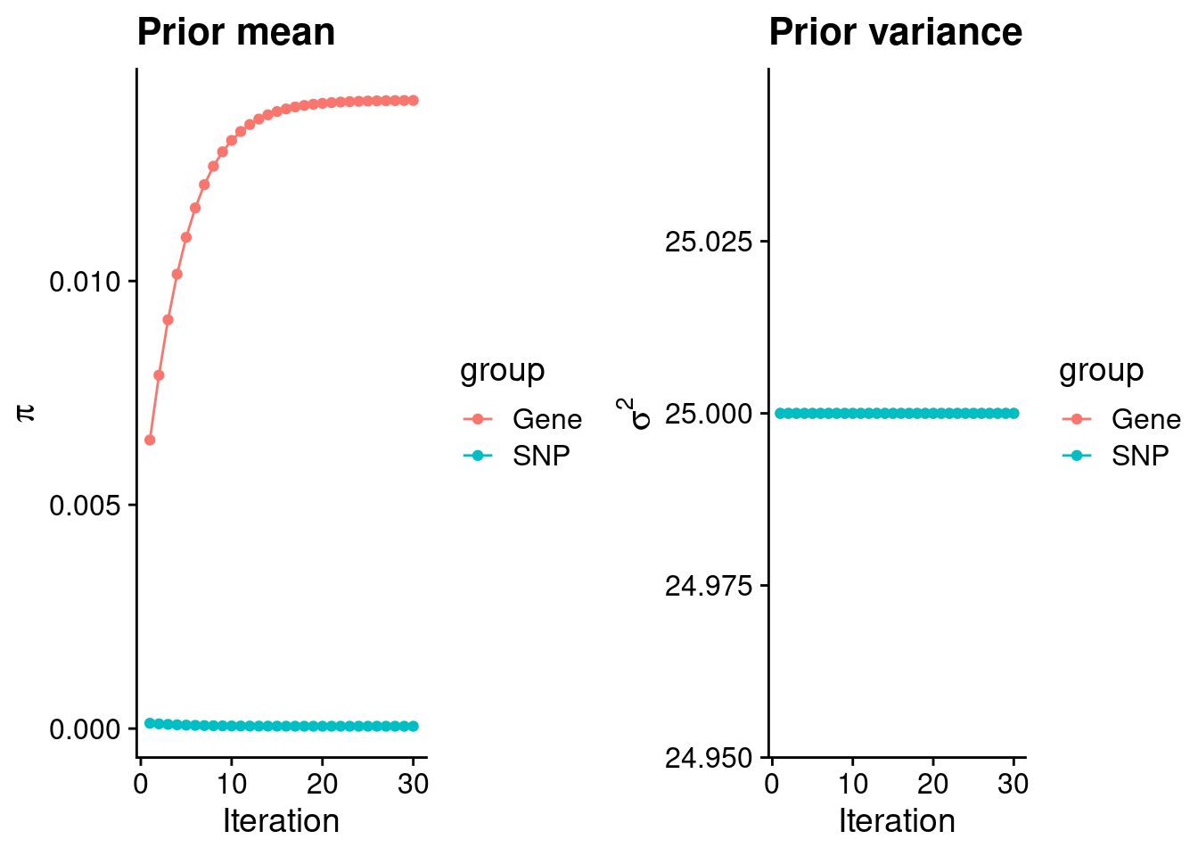
| Version | Author | Date |
|---|---|---|
| b14741c | wesleycrouse | 2021-09-06 |
#estimated group prior
estimated_group_prior <- group_prior_rec[,ncol(group_prior_rec)]
names(estimated_group_prior) <- c("gene", "snp")
estimated_group_prior["snp"] <- estimated_group_prior["snp"]*thin #adjust parameter to account for thin argument
print(estimated_group_prior)
gene snp
1.403410e-02 5.189707e-05 #estimated group prior variance
estimated_group_prior_var <- group_prior_var_rec[,ncol(group_prior_var_rec)]
names(estimated_group_prior_var) <- c("gene", "snp")
print(estimated_group_prior_var)gene snp
25 25 #report sample size
print(sample_size)[1] 292933#report group size
group_size <- c(nrow(ctwas_gene_res), n_snps)
print(group_size)[1] 10901 8697330#estimated group PVE
estimated_group_pve <- estimated_group_prior_var*estimated_group_prior*group_size/sample_size #check PVE calculation
names(estimated_group_pve) <- c("gene", "snp")
print(estimated_group_pve) gene snp
0.01305638 0.03852126 #compare sum(PIP*mu2/sample_size) with above PVE calculation
c(sum(ctwas_gene_res$PVE),sum(ctwas_snp_res$PVE))[1] 0.02927078 0.66913463Genes with highest PIPs
#distribution of PIPs
hist(ctwas_gene_res$susie_pip, xlim=c(0,1), main="Distribution of Gene PIPs")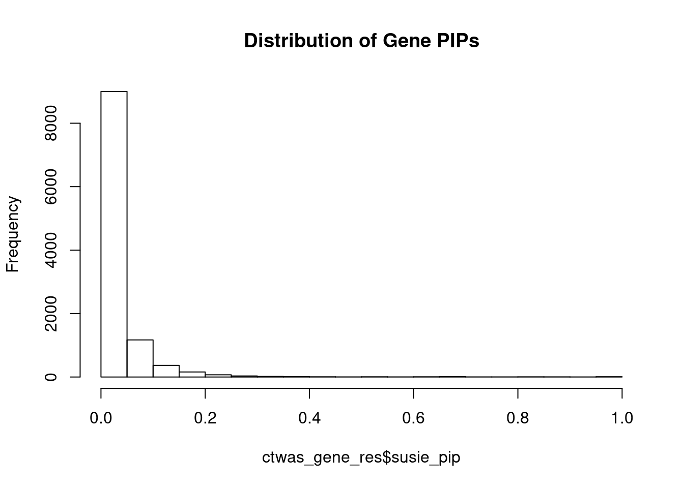
| Version | Author | Date |
|---|---|---|
| b14741c | wesleycrouse | 2021-09-06 |
#genes with PIP>0.8 or 20 highest PIPs
head(ctwas_gene_res[order(-ctwas_gene_res$susie_pip),report_cols], max(sum(ctwas_gene_res$susie_pip>0.8), 20))
genename region_tag susie_pip mu2 PVE z
3212 CCND2 12_4 0.996 31.33 1.1e-04 5.34
12467 RP11-219B17.3 15_27 0.995 52.81 1.8e-04 7.18
7040 INHBB 2_70 0.988 26.35 8.9e-05 4.81
1320 CWF19L1 10_64 0.979 32.02 1.1e-04 -7.09
3562 ACVR1C 2_94 0.972 24.89 8.3e-05 4.62
5563 ABCG8 2_27 0.971 37.02 1.2e-04 5.88
11790 CYP2A6 19_28 0.959 24.54 8.0e-05 -4.73
4269 ITGB4 17_42 0.957 22.69 7.4e-05 -4.91
2359 ABCC3 17_29 0.951 22.33 7.2e-05 4.38
1848 CD276 15_35 0.925 39.20 1.2e-04 6.13
1120 CETP 16_31 0.908 20.46 6.3e-05 -4.03
10667 HLA-G 6_24 0.889 1334.32 4.0e-03 -6.69
12687 RP4-781K5.7 1_121 0.888 21.46 6.5e-05 -4.17
10495 PRMT6 1_66 0.887 29.83 9.0e-05 5.14
10212 IL27 16_23 0.874 26.19 7.8e-05 -4.76
2924 EFHD1 2_136 0.856 30.41 8.9e-05 6.05
1231 PABPC4 1_24 0.844 24.64 7.1e-05 4.52
5978 ZC3H12C 11_65 0.843 21.64 6.2e-05 -4.19
1146 DNMT3B 20_19 0.840 20.73 5.9e-05 -3.98
537 DGAT2 11_42 0.813 57.18 1.6e-04 -7.51
1153 TGDS 13_47 0.809 20.66 5.7e-05 -4.00
11669 RP11-452H21.4 11_43 0.805 36.15 9.9e-05 5.78Genes with largest effect sizes
#plot PIP vs effect size
plot(ctwas_gene_res$susie_pip, ctwas_gene_res$mu2, xlab="PIP", ylab="mu^2", main="Gene PIPs vs Effect Size")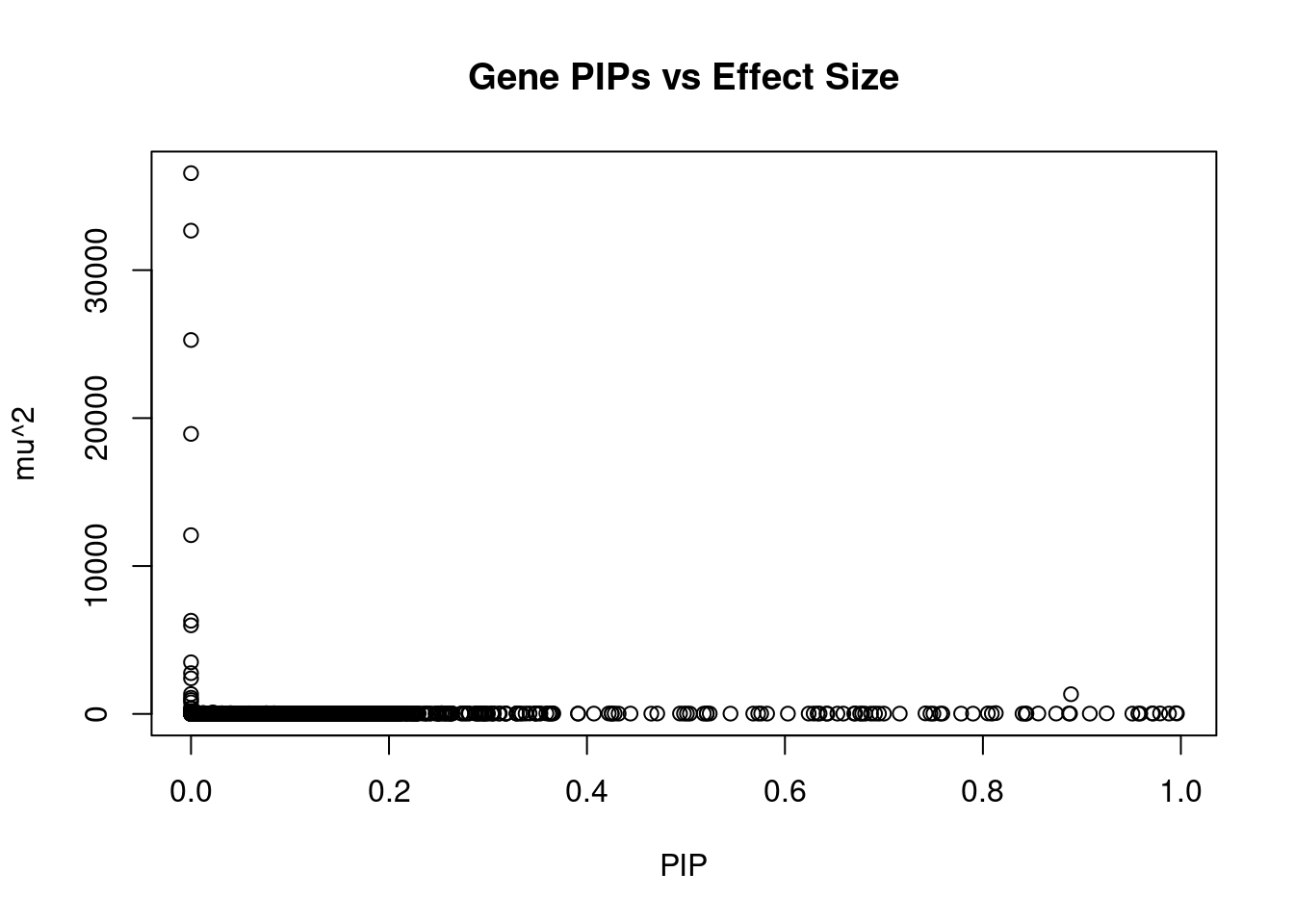
| Version | Author | Date |
|---|---|---|
| b14741c | wesleycrouse | 2021-09-06 |
#genes with 20 largest effect sizes
head(ctwas_gene_res[order(-ctwas_gene_res$mu2),report_cols],20)
genename region_tag susie_pip mu2 PVE z
11533 UGT1A4 2_137 0.000 36556.51 0.0e+00 232.75
11447 UGT1A1 2_137 0.000 32669.69 0.0e+00 -230.41
11489 UGT1A3 2_137 0.000 25276.37 0.0e+00 213.80
7732 UGT1A6 2_137 0.000 18932.93 0.0e+00 186.96
12683 HCP5B 6_24 0.000 12085.12 1.0e-07 -3.52
10663 TRIM31 6_24 0.000 6301.01 1.1e-11 1.07
4833 FLOT1 6_24 0.000 5989.52 9.6e-12 -1.07
11522 UGT1A7 2_137 0.000 3491.57 0.0e+00 -71.90
10651 ABCF1 6_24 0.000 2758.70 1.9e-09 -3.76
5766 PPP1R18 6_24 0.000 2404.67 3.3e-09 -3.94
4836 NRM 6_24 0.000 1343.59 5.4e-13 -0.40
10667 HLA-G 6_24 0.889 1334.32 4.0e-03 -6.69
1088 USP40 2_137 0.000 1095.76 0.0e+00 -46.64
624 ZNRD1 6_24 0.000 946.03 4.6e-13 0.19
10747 SLCO1B7 12_16 0.000 784.97 0.0e+00 12.26
10661 TRIM10 6_24 0.000 401.91 1.7e-13 -0.49
2584 SLCO1B3 12_16 0.000 360.97 0.0e+00 9.93
4482 SPX 12_16 0.000 189.40 0.0e+00 4.60
10648 C6orf136 6_24 0.000 179.57 7.5e-14 0.11
11136 HCG20 6_24 0.000 175.76 4.8e-13 -1.98Genes with highest PVE
#genes with 20 highest pve
head(ctwas_gene_res[order(-ctwas_gene_res$PVE),report_cols],20)
genename region_tag susie_pip mu2 PVE z
10667 HLA-G 6_24 0.889 1334.32 4.0e-03 -6.69
12467 RP11-219B17.3 15_27 0.995 52.81 1.8e-04 7.18
537 DGAT2 11_42 0.813 57.18 1.6e-04 -7.51
5563 ABCG8 2_27 0.971 37.02 1.2e-04 5.88
1848 CD276 15_35 0.925 39.20 1.2e-04 6.13
1320 CWF19L1 10_64 0.979 32.02 1.1e-04 -7.09
3212 CCND2 12_4 0.996 31.33 1.1e-04 5.34
11669 RP11-452H21.4 11_43 0.805 36.15 9.9e-05 5.78
2004 TGFB1 19_28 0.742 38.56 9.8e-05 5.64
10495 PRMT6 1_66 0.887 29.83 9.0e-05 5.14
7040 INHBB 2_70 0.988 26.35 8.9e-05 4.81
2924 EFHD1 2_136 0.856 30.41 8.9e-05 6.05
3562 ACVR1C 2_94 0.972 24.89 8.3e-05 4.62
11790 CYP2A6 19_28 0.959 24.54 8.0e-05 -4.73
10212 IL27 16_23 0.874 26.19 7.8e-05 -4.76
8142 CNTROB 17_7 0.671 33.12 7.6e-05 -5.71
4269 ITGB4 17_42 0.957 22.69 7.4e-05 -4.91
2359 ABCC3 17_29 0.951 22.33 7.2e-05 4.38
1231 PABPC4 1_24 0.844 24.64 7.1e-05 4.52
6093 CSNK1G3 5_75 0.759 25.56 6.6e-05 4.74Genes with largest z scores
#genes with 20 largest z scores
head(ctwas_gene_res[order(-abs(ctwas_gene_res$z)),report_cols],20)
genename region_tag susie_pip mu2 PVE z
11533 UGT1A4 2_137 0.000 36556.51 0.0e+00 232.75
11447 UGT1A1 2_137 0.000 32669.69 0.0e+00 -230.41
11489 UGT1A3 2_137 0.000 25276.37 0.0e+00 213.80
7732 UGT1A6 2_137 0.000 18932.93 0.0e+00 186.96
11522 UGT1A7 2_137 0.000 3491.57 0.0e+00 -71.90
1088 USP40 2_137 0.000 1095.76 0.0e+00 -46.64
10747 SLCO1B7 12_16 0.000 784.97 0.0e+00 12.26
3556 HJURP 2_137 0.000 122.43 0.0e+00 10.96
8651 MSL2 3_84 0.022 104.80 7.9e-06 10.28
2584 SLCO1B3 12_16 0.000 360.97 0.0e+00 9.93
2586 GOLT1B 12_16 0.000 78.22 0.0e+00 7.53
537 DGAT2 11_42 0.813 57.18 1.6e-04 -7.51
11290 MAPKAPK5-AS1 12_67 0.040 54.00 7.3e-06 -7.21
12467 RP11-219B17.3 15_27 0.995 52.81 1.8e-04 7.18
2541 ALDH2 12_67 0.031 51.20 5.5e-06 7.10
1320 CWF19L1 10_64 0.979 32.02 1.1e-04 -7.09
2536 SH2B3 12_67 0.011 42.12 1.6e-06 6.80
10667 HLA-G 6_24 0.889 1334.32 4.0e-03 -6.69
2170 AHR 7_17 0.013 39.39 1.7e-06 -6.58
4962 EXOC6 10_59 0.024 54.35 4.4e-06 -6.37Comparing z scores and PIPs
#set nominal signifiance threshold for z scores
alpha <- 0.05

#bonferroni adjusted threshold for z scores
sig_thresh <- qnorm(1-(alpha/nrow(ctwas_gene_res)/2), lower=T)

#Q-Q plot for z scores
obs_z <- ctwas_gene_res$z[order(ctwas_gene_res$z)]
exp_z <- qnorm((1:nrow(ctwas_gene_res))/nrow(ctwas_gene_res))

plot(exp_z, obs_z, xlab="Expected z", ylab="Observed z", main="Gene z score Q-Q plot")
abline(a=0,b=1)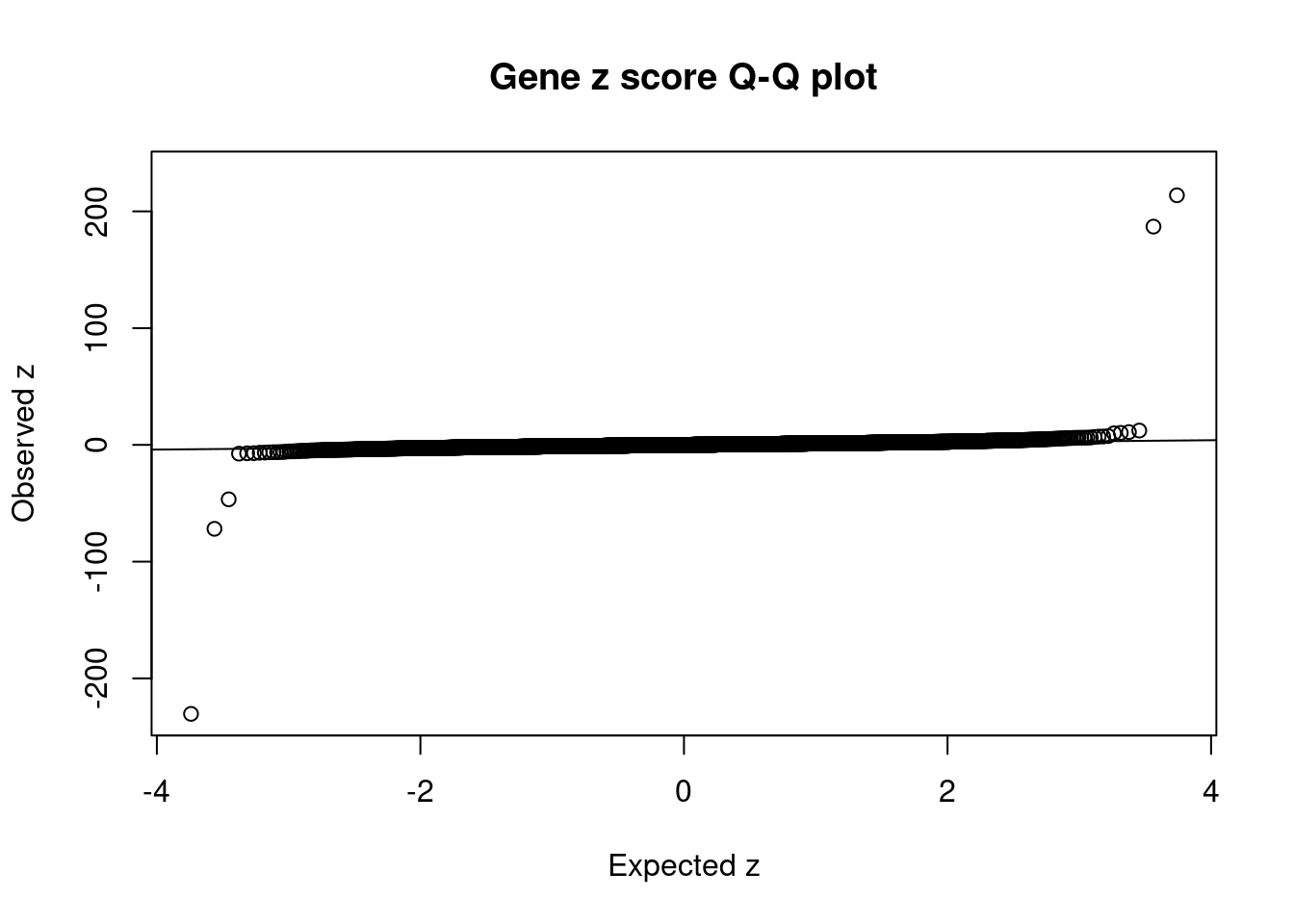
| Version | Author | Date |
|---|---|---|
| b14741c | wesleycrouse | 2021-09-06 |
#plot z score vs PIP
plot(abs(ctwas_gene_res$z), ctwas_gene_res$susie_pip, xlab="abs(z)", ylab="PIP")
abline(v=sig_thresh, col="red", lty=2)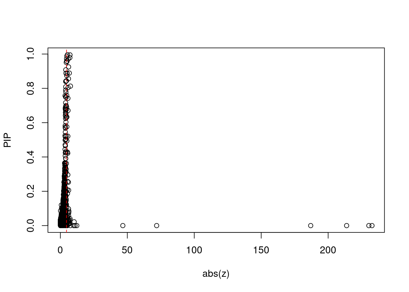
| Version | Author | Date |
|---|---|---|
| b14741c | wesleycrouse | 2021-09-06 |
#proportion of significant z scores
mean(abs(ctwas_gene_res$z) > sig_thresh)
[1] 0.006696633#genes with most significant z scores
head(ctwas_gene_res[order(-abs(ctwas_gene_res$z)),report_cols],20) genename region_tag susie_pip mu2 PVE z
11533 UGT1A4 2_137 0.000 36556.51 0.0e+00 232.75
11447 UGT1A1 2_137 0.000 32669.69 0.0e+00 -230.41
11489 UGT1A3 2_137 0.000 25276.37 0.0e+00 213.80
7732 UGT1A6 2_137 0.000 18932.93 0.0e+00 186.96
11522 UGT1A7 2_137 0.000 3491.57 0.0e+00 -71.90
1088 USP40 2_137 0.000 1095.76 0.0e+00 -46.64
10747 SLCO1B7 12_16 0.000 784.97 0.0e+00 12.26
3556 HJURP 2_137 0.000 122.43 0.0e+00 10.96
8651 MSL2 3_84 0.022 104.80 7.9e-06 10.28
2584 SLCO1B3 12_16 0.000 360.97 0.0e+00 9.93
2586 GOLT1B 12_16 0.000 78.22 0.0e+00 7.53
537 DGAT2 11_42 0.813 57.18 1.6e-04 -7.51
11290 MAPKAPK5-AS1 12_67 0.040 54.00 7.3e-06 -7.21
12467 RP11-219B17.3 15_27 0.995 52.81 1.8e-04 7.18
2541 ALDH2 12_67 0.031 51.20 5.5e-06 7.10
1320 CWF19L1 10_64 0.979 32.02 1.1e-04 -7.09
2536 SH2B3 12_67 0.011 42.12 1.6e-06 6.80
10667 HLA-G 6_24 0.889 1334.32 4.0e-03 -6.69
2170 AHR 7_17 0.013 39.39 1.7e-06 -6.58
4962 EXOC6 10_59 0.024 54.35 4.4e-06 -6.37Locus plots for genes and SNPs
ctwas_gene_res_sortz <- ctwas_gene_res[order(-abs(ctwas_gene_res$z)),]

n_plots <- 5
for (region_tag_plot in head(unique(ctwas_gene_res_sortz$region_tag), n_plots)){
  ctwas_res_region <-  ctwas_res[ctwas_res$region_tag==region_tag_plot,]
  start <- min(ctwas_res_region$pos)
  end <- max(ctwas_res_region$pos)

  ctwas_res_region <- ctwas_res_region[order(ctwas_res_region$pos),]
  ctwas_res_region_gene <- ctwas_res_region[ctwas_res_region$type=="gene",]
  ctwas_res_region_snp <- ctwas_res_region[ctwas_res_region$type=="SNP",]

  #region name
  print(paste0("Region: ", region_tag_plot))

  #table of genes in region
  print(ctwas_res_region_gene[,report_cols])

  par(mfrow=c(4,1))

  #gene z scores
  plot(ctwas_res_region_gene$pos, abs(ctwas_res_region_gene$z), xlab="Position", ylab="abs(gene_z)", xlim=c(start,end),
   ylim=c(0,max(sig_thresh, abs(ctwas_res_region_gene$z))),
   main=paste0("Region: ", region_tag_plot))
  abline(h=sig_thresh,col="red",lty=2)

  #significance threshold for SNPs
  alpha_snp <- 5*10^(-8)
  sig_thresh_snp <- qnorm(1-alpha_snp/2, lower=T)

  #snp z scores
  plot(ctwas_res_region_snp$pos, abs(ctwas_res_region_snp$z), xlab="Position", ylab="abs(snp_z)",xlim=c(start,end),
   ylim=c(0,max(sig_thresh_snp, max(abs(ctwas_res_region_snp$z)))))
  abline(h=sig_thresh_snp,col="purple",lty=2)

  #gene pips
  plot(ctwas_res_region_gene$pos, ctwas_res_region_gene$susie_pip, xlab="Position", ylab="Gene PIP", xlim=c(start,end), ylim=c(0,1))
  abline(h=0.8,col="blue",lty=2)

  #snp pips
  plot(ctwas_res_region_snp$pos, ctwas_res_region_snp$susie_pip, xlab="Position", ylab="SNP PIP", xlim=c(start,end), ylim=c(0,1))
  abline(h=0.8,col="blue",lty=2)
}
[1] "Region: 2_137"
genename region_tag susie_pip mu2 PVE z
10567 GIGYF2 2_137 0 19.52 0 -5.12
9340 C2orf82 2_137 0 5.77 0 0.45
620 NGEF 2_137 0 9.06 0 2.52
8006 INPP5D 2_137 0 12.51 0 4.05
879 DGKD 2_137 0 30.48 0 -0.07
1088 USP40 2_137 0 1095.76 0 -46.64
11522 UGT1A7 2_137 0 3491.57 0 -71.90
7732 UGT1A6 2_137 0 18932.93 0 186.96
11533 UGT1A4 2_137 0 36556.51 0 232.75
11489 UGT1A3 2_137 0 25276.37 0 213.80
11447 UGT1A1 2_137 0 32669.69 0 -230.41
3556 HJURP 2_137 0 122.43 0 10.96
11098 AC006037.2 2_137 0 5.39 0 1.50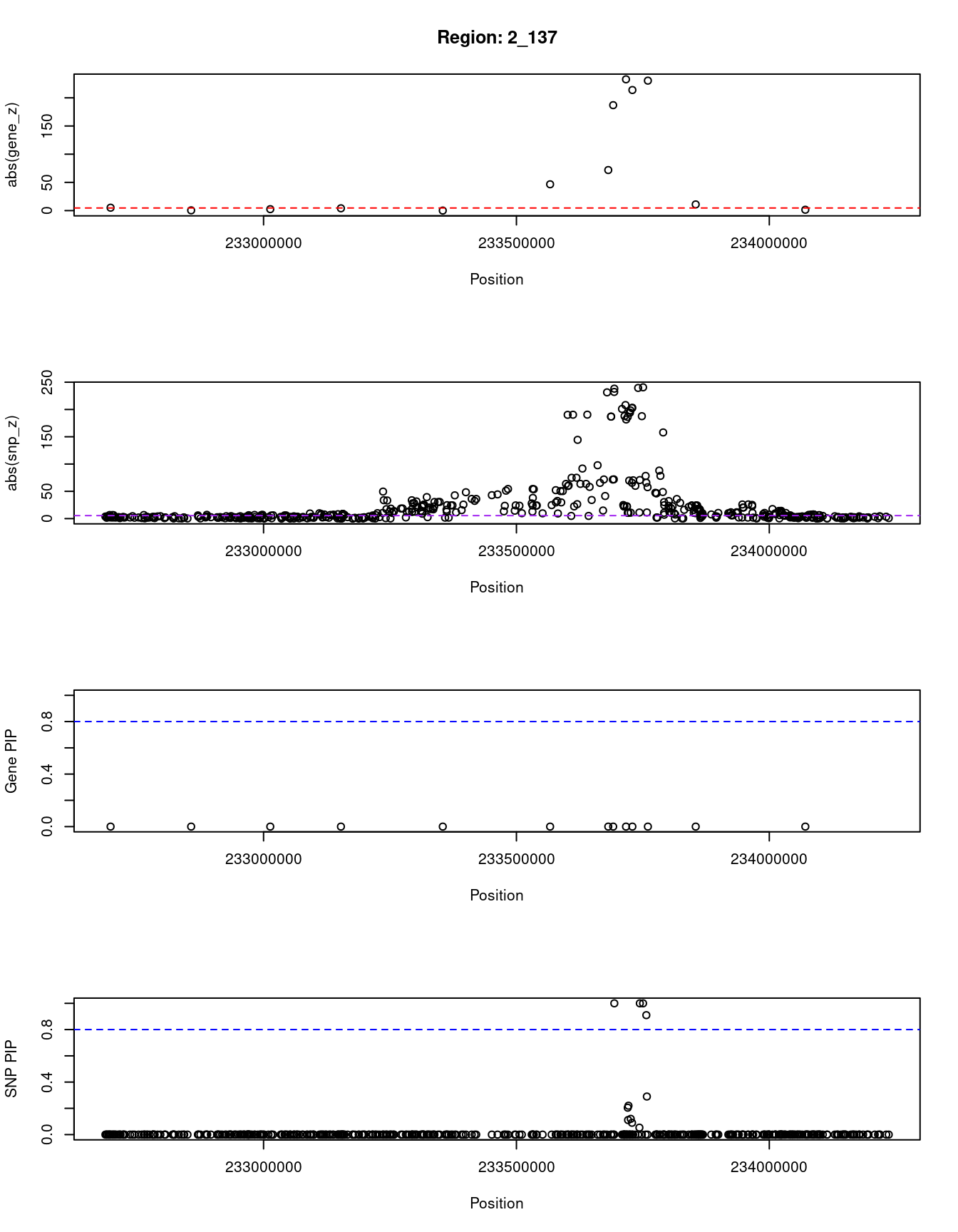
| Version | Author | Date |
|---|---|---|
| b14741c | wesleycrouse | 2021-09-06 |
[1] "Region: 12_16"
      genename region_tag susie_pip    mu2 PVE     z
2584   SLCO1B3      12_16         0 360.97   0  9.93
10747  SLCO1B7      12_16         0 784.97   0 12.26
3400      IAPP      12_16         0 120.32   0  5.16
3399   PYROXD1      12_16         0  14.39   0  0.89
36       RECQL      12_16         0 161.81   0  3.81
2586    GOLT1B      12_16         0  78.22   0  7.53
4482       SPX      12_16         0 189.40   0  4.60
2587      LDHB      12_16         0  10.00   0  0.07
3401     KCNJ8      12_16         0   7.08   0 -0.33
689      ABCC9      12_16         0   8.22   0  2.11
2590     C2CD5      12_16         0  12.46   0 -1.39
5073     ETNK1      12_16         0  10.83   0  0.30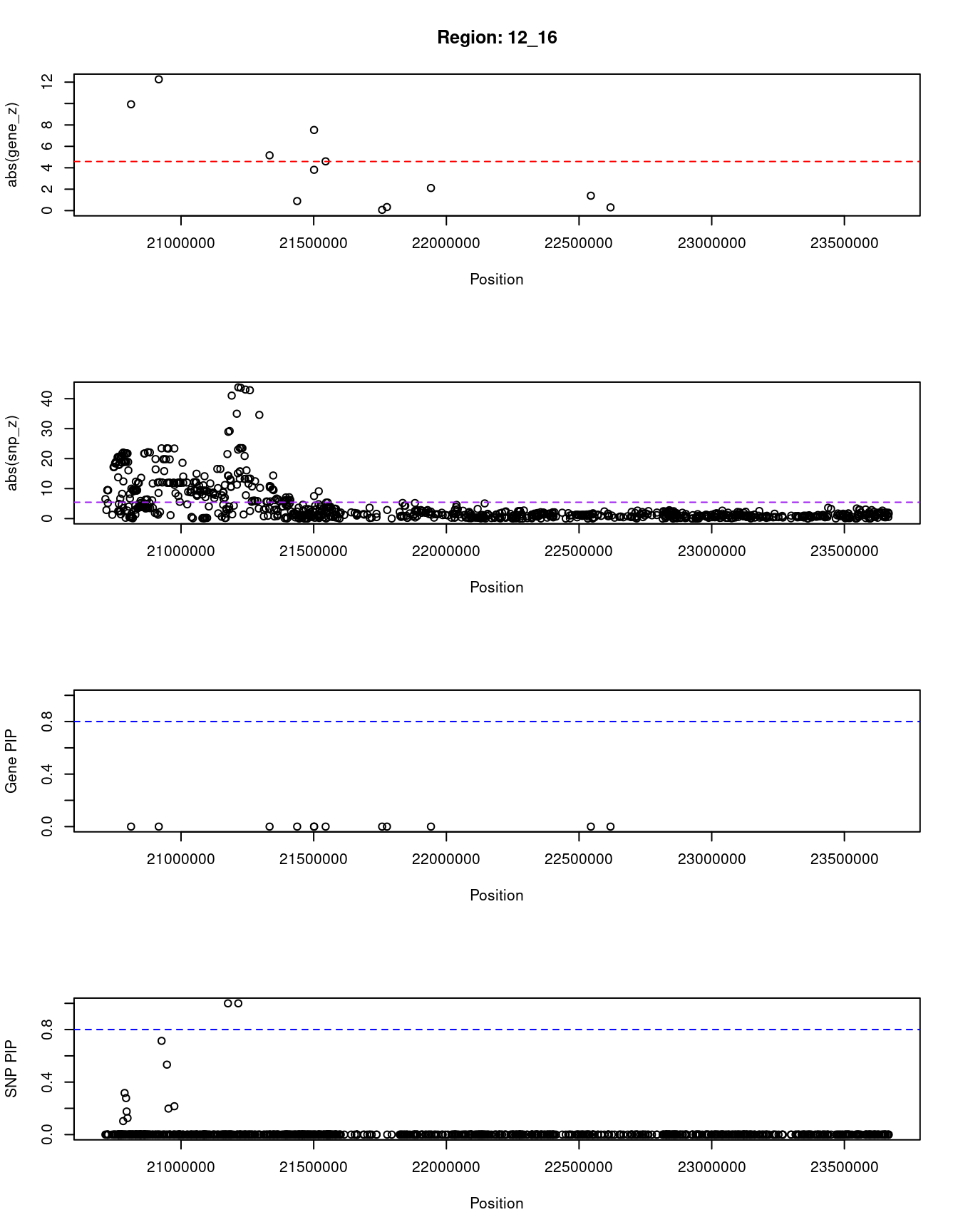
| Version | Author | Date |
|---|---|---|
| b14741c | wesleycrouse | 2021-09-06 |
[1] "Region: 3_84"
     genename region_tag susie_pip    mu2     PVE     z
796   PPP2R3A       3_84     0.041  18.33 2.6e-06 -2.46
8651     MSL2       3_84     0.022 104.80 7.9e-06 10.28
2795     PCCB       3_84     0.014   6.33 3.1e-07  1.22
3148    STAG1       3_84     0.015   5.19 2.6e-07 -0.03
6584     NCK1       3_84     0.014   9.46 4.6e-07 -2.19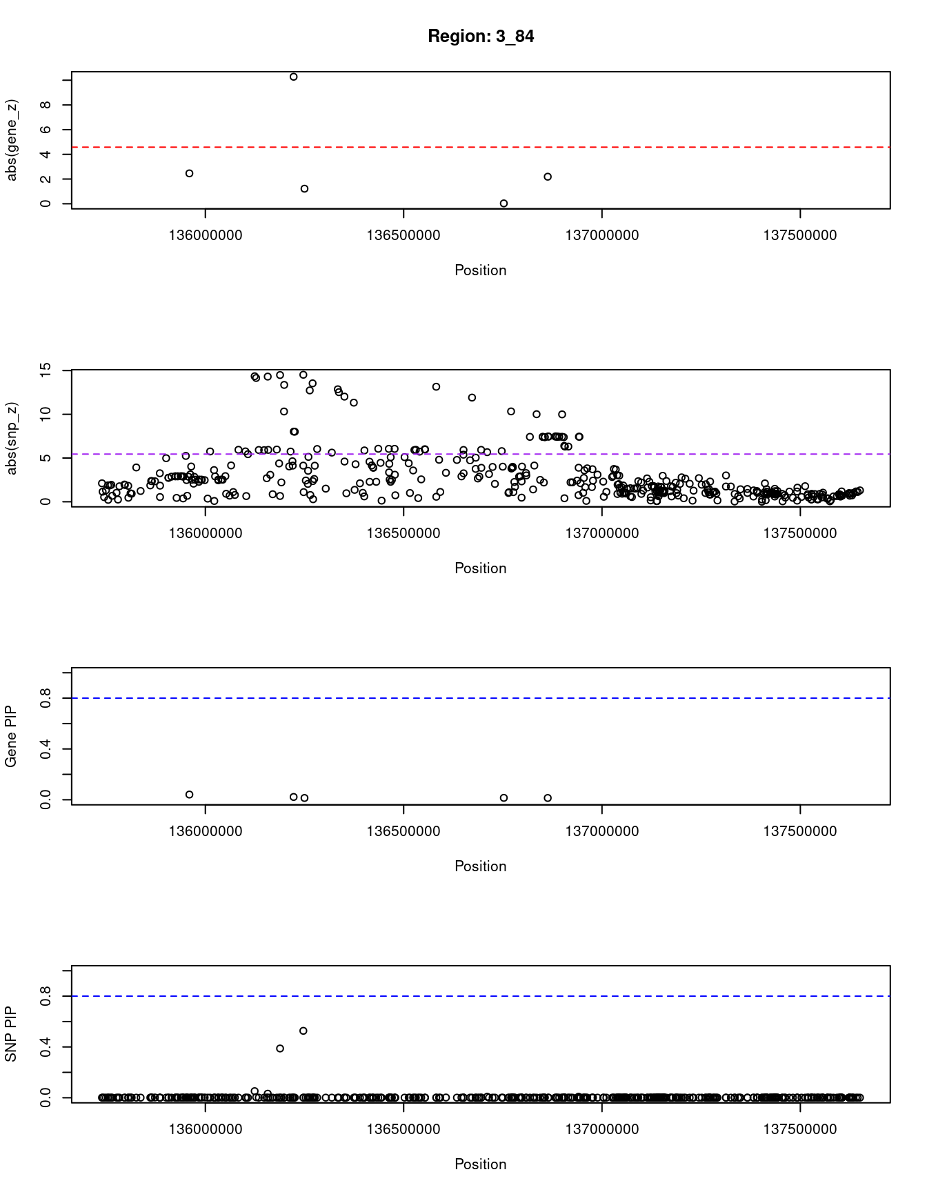
| Version | Author | Date |
|---|---|---|
| b14741c | wesleycrouse | 2021-09-06 |
[1] "Region: 11_42"
           genename region_tag susie_pip   mu2     PVE     z
7611          XRRA1      11_42     0.026  9.38 8.5e-07 -1.00
3170          SPCS2      11_42     0.019  6.48 4.2e-07  0.73
6901           NEU3      11_42     0.017  5.04 2.9e-07  0.39
4848        SLCO2B1      11_42     0.017  5.06 2.9e-07 -0.22
12001         TPBGL      11_42     0.023  7.94 6.3e-07  0.68
6617          GDPD5      11_42     0.024 11.38 9.5e-07  1.95
8328           MAP6      11_42     0.022  7.34 5.6e-07  0.24
7603         MOGAT2      11_42     0.102 19.48 6.8e-06  0.85
537           DGAT2      11_42     0.813 57.18 1.6e-04 -7.51
10381         UVRAG      11_42     0.019  8.07 5.4e-07  1.62
1082          WNT11      11_42     0.025  8.98 7.5e-07  1.06
11773 RP11-619A14.3      11_42     0.019  6.36 4.2e-07  0.61
4849         THAP12      11_42     0.018  6.01 3.7e-07 -0.66
12265 RP11-111M22.5      11_42     0.020  7.06 4.9e-07  0.80
11766 RP11-111M22.3      11_42     0.017  5.05 2.9e-07  0.31
11751  RP11-672A2.4      11_42     0.018  5.92 3.7e-07  0.53
9350           TSKU      11_42     0.018  5.57 3.4e-07  0.25
905           ACER3      11_42     0.083 20.30 5.7e-06 -2.04
5976          CAPN5      11_42     0.052 16.31 2.9e-06  1.72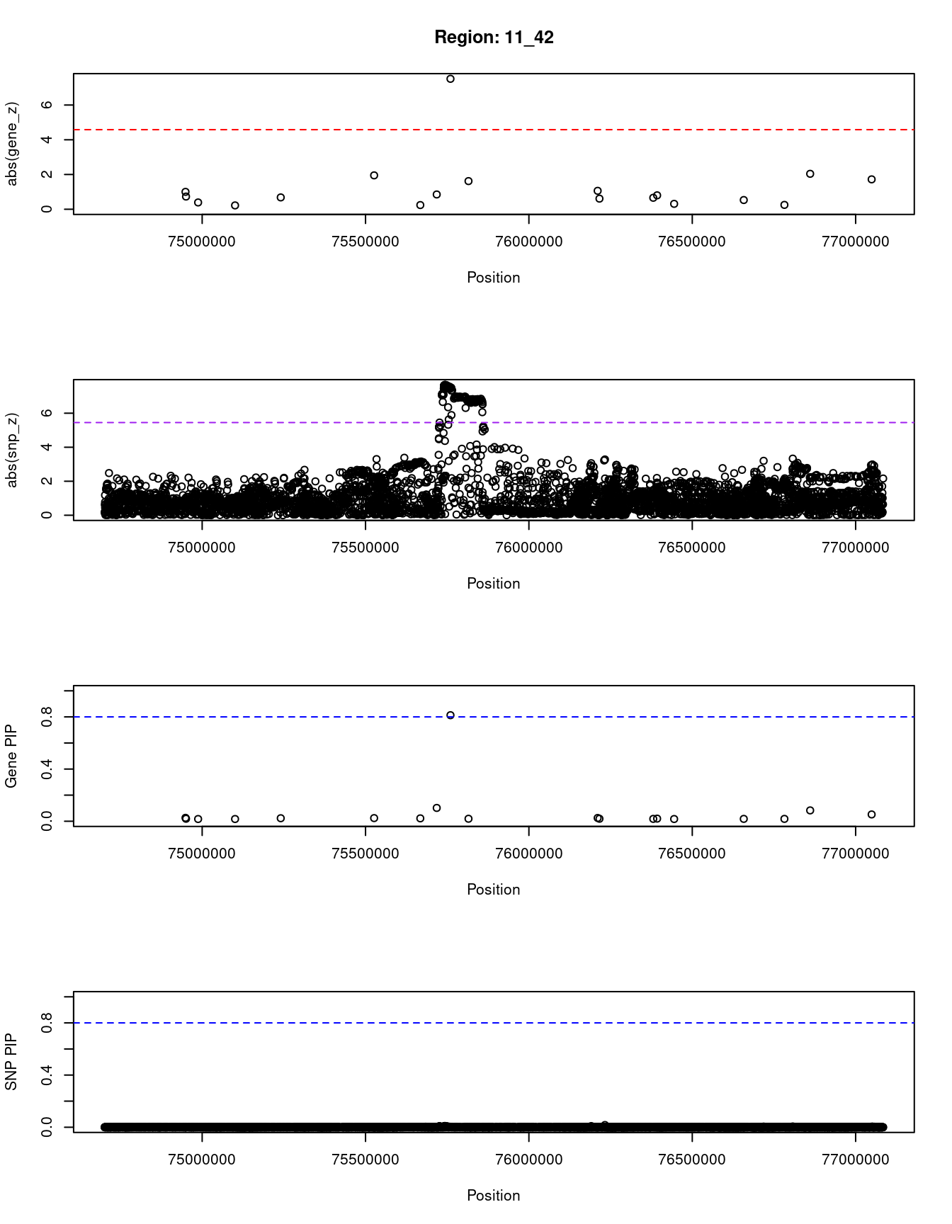
| Version | Author | Date |
|---|---|---|
| b14741c | wesleycrouse | 2021-09-06 |
[1] "Region: 12_67"
          genename region_tag susie_pip   mu2     PVE     z
5112          TCHP      12_67     0.334 18.64 2.1e-05  3.21
5111          GIT2      12_67     0.193 17.49 1.2e-05  3.36
8639      C12orf76      12_67     0.014  7.16 3.5e-07 -0.30
3515         IFT81      12_67     0.016 12.26 6.6e-07  2.50
10093       ANAPC7      12_67     0.017 10.87 6.3e-07  2.16
2531         ARPC3      12_67     0.018  8.90 5.5e-07  0.54
10684      FAM216A      12_67     0.013 10.38 4.7e-07  2.42
2532          GPN3      12_67     0.011  6.09 2.3e-07  1.40
2533         VPS29      12_67     0.011  6.16 2.4e-07 -1.41
10683        TCTN1      12_67     0.015  7.13 3.7e-07  0.02
3517         HVCN1      12_67     0.029 16.92 1.7e-06  2.67
9717        PPP1CC      12_67     0.029 16.84 1.7e-06 -2.65
10375      FAM109A      12_67     0.011  8.05 3.1e-07 -1.46
2536         SH2B3      12_67     0.011 42.12 1.6e-06  6.80
10680        ATXN2      12_67     0.011 20.51 7.8e-07  3.97
2541         ALDH2      12_67     0.031 51.20 5.5e-06  7.10
11290 MAPKAPK5-AS1      12_67     0.040 54.00 7.3e-06 -7.21
1191         ERP29      12_67     0.076 46.69 1.2e-05  6.25
10370      TMEM116      12_67     0.076 46.69 1.2e-05 -6.25
2544         NAA25      12_67     0.059 43.51 8.8e-06 -6.12
8505        HECTD4      12_67     0.084 49.39 1.4e-05  6.33
9084        PTPN11      12_67     0.015  7.99 4.2e-07 -0.78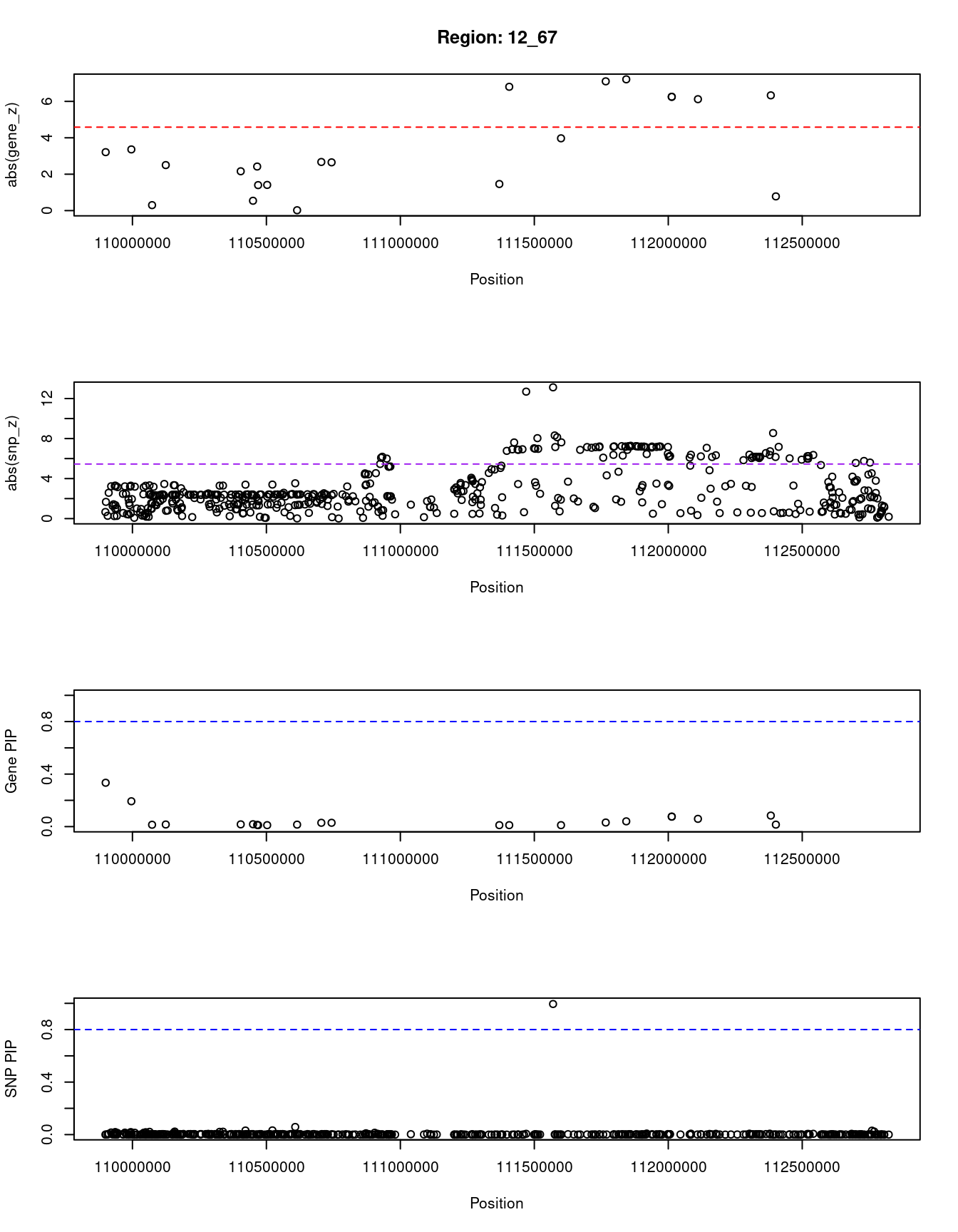
| Version | Author | Date |
|---|---|---|
| b14741c | wesleycrouse | 2021-09-06 |
SNPs with highest PIPs
#snps with PIP>0.8 or 20 highest PIPs
head(ctwas_snp_res[order(-ctwas_snp_res$susie_pip),report_cols_snps],
max(sum(ctwas_snp_res$susie_pip>0.8), 20))
id region_tag susie_pip mu2 PVE z
132828 rs2070959 2_137 1.000 28459.01 9.7e-02 238.14
132856 rs76063448 2_137 1.000 5888.78 2.0e-02 70.66
132858 rs2885296 2_137 1.000 40201.66 1.4e-01 240.61
327685 rs72834643 6_20 1.000 119.90 4.1e-04 9.73
327706 rs115740542 6_20 1.000 180.33 6.2e-04 12.66
371809 rs12208357 6_103 1.000 80.44 2.7e-04 -6.65
383595 rs542176135 7_17 1.000 152.49 5.2e-04 -8.38
534815 rs6480402 10_46 1.000 463.77 1.6e-03 8.90
604087 rs11045819 12_16 1.000 2525.87 8.6e-03 -14.34
604104 rs4363657 12_16 1.000 1587.00 5.4e-03 43.78
799284 rs59616136 19_14 1.000 49.30 1.7e-04 7.00
891763 rs13031505 2_136 1.000 59.39 2.0e-04 -8.07
895089 rs1611236 6_24 1.000 25202.51 8.6e-02 -3.60
328548 rs3130253 6_23 0.999 41.00 1.4e-04 -6.63
510100 rs115478735 9_70 0.999 64.59 2.2e-04 -8.02
807430 rs113345881 19_32 0.999 38.14 1.3e-04 6.12
807428 rs814573 19_32 0.998 37.40 1.3e-04 -6.68
556111 rs76153913 11_2 0.997 47.81 1.6e-04 6.70
383617 rs4721597 7_17 0.996 88.59 3.0e-04 1.94
614777 rs7397189 12_36 0.995 34.89 1.2e-04 5.69
631363 rs653178 12_67 0.995 160.56 5.5e-04 -13.12
891700 rs34247311 2_136 0.995 38.70 1.3e-04 4.44
819161 rs34507316 20_13 0.993 32.86 1.1e-04 5.60
797513 rs141645070 19_10 0.989 30.06 1.0e-04 -5.27
36470 rs2779116 1_78 0.980 68.69 2.3e-04 -8.25
746176 rs2608604 16_53 0.972 55.49 1.8e-04 -6.33
807433 rs12721109 19_32 0.972 31.43 1.0e-04 6.44
800069 rs3794991 19_15 0.952 132.20 4.3e-04 11.64
807364 rs1551891 19_32 0.949 34.75 1.1e-04 7.88
234586 rs17238095 4_72 0.938 29.18 9.3e-05 5.18
847467 rs34662558 22_10 0.930 30.49 9.7e-05 -5.19
603802 rs7962574 12_15 0.921 45.83 1.4e-04 -8.40
496018 rs9410381 9_45 0.913 74.38 2.3e-04 8.62
132860 rs11568318 2_137 0.910 1443.19 4.5e-03 -65.81
510485 rs34755157 9_71 0.900 28.91 8.9e-05 -5.03
438526 rs12549737 8_24 0.898 30.01 9.2e-05 5.15
560564 rs34623292 11_10 0.892 29.87 9.1e-05 -5.06
603807 rs73080739 12_15 0.887 33.82 1.0e-04 -7.24
327524 rs75080831 6_19 0.851 59.63 1.7e-04 7.96
295901 rs4566840 5_66 0.849 31.75 9.2e-05 -5.46
603842 rs10770693 12_15 0.849 59.16 1.7e-04 8.86
850218 rs6000553 22_14 0.840 43.93 1.3e-04 6.47
559133 rs4910498 11_8 0.832 50.78 1.4e-04 6.71
73907 rs780093 2_16 0.813 37.31 1.0e-04 5.98SNPs with largest effect sizes
#plot PIP vs effect size
plot(ctwas_snp_res$susie_pip, ctwas_snp_res$mu2, xlab="PIP", ylab="mu^2", main="SNP PIPs vs Effect Size")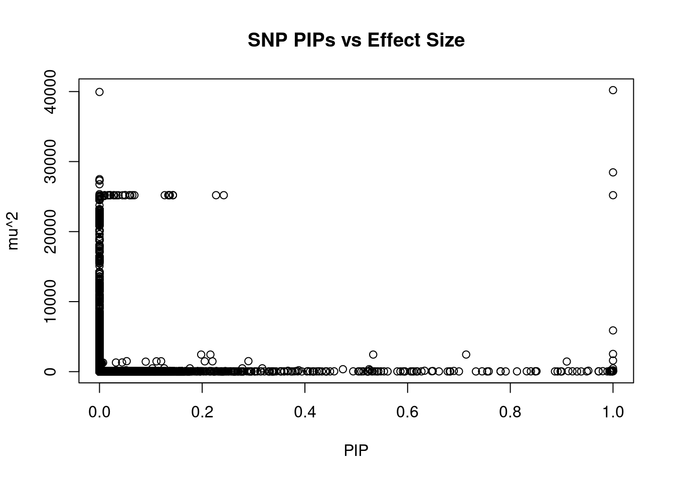
| Version | Author | Date |
|---|---|---|
| b14741c | wesleycrouse | 2021-09-06 |
#SNPs with 50 largest effect sizes
head(ctwas_snp_res[order(-ctwas_snp_res$mu2),report_cols_snps],50)
id region_tag susie_pip mu2 PVE z
132858 rs2885296 2_137 1.000 40201.66 1.4e-01 240.61
132854 rs17862875 2_137 0.000 39943.84 0.0e+00 239.53
132828 rs2070959 2_137 1.000 28459.01 9.7e-02 238.14
132827 rs1105880 2_137 0.000 27491.08 0.0e+00 232.16
132822 rs77070100 2_137 0.000 27306.28 0.0e+00 231.38
132857 rs11888459 2_137 0.000 27291.21 0.0e+00 187.72
132840 rs13401281 2_137 0.000 26765.91 0.0e+00 186.34
132836 rs6749496 2_137 0.000 25345.04 0.0e+00 208.13
895089 rs1611236 6_24 1.000 25202.51 8.6e-02 -3.60
895112 rs1611248 6_24 0.227 25201.43 1.9e-02 -3.63
895116 rs1611252 6_24 0.137 25201.31 1.2e-02 -3.62
895071 rs111734624 6_24 0.143 25201.27 1.2e-02 -3.62
895068 rs2508055 6_24 0.143 25201.26 1.2e-02 -3.62
895133 rs1611260 6_24 0.135 25201.25 1.2e-02 -3.62
895139 rs1611265 6_24 0.134 25201.23 1.1e-02 -3.62
895007 rs1633033 6_24 0.242 25201.13 2.1e-02 -3.63
895020 rs2844838 6_24 0.127 25200.67 1.1e-02 -3.63
895141 rs1611267 6_24 0.058 25200.63 5.0e-03 -3.62
895143 rs2394171 6_24 0.050 25200.60 4.3e-03 -3.61
895145 rs2893981 6_24 0.050 25200.55 4.3e-03 -3.61
895075 rs1611228 6_24 0.064 25200.49 5.5e-03 -3.62
895064 rs1737020 6_24 0.021 25200.05 1.8e-03 -3.60
895065 rs1737019 6_24 0.021 25200.05 1.8e-03 -3.60
895024 rs1633032 6_24 0.068 25198.93 5.8e-03 -3.62
895058 rs1633020 6_24 0.027 25197.30 2.4e-03 -3.61
895062 rs1633018 6_24 0.010 25196.74 8.4e-04 -3.60
895087 rs1611234 6_24 0.010 25195.27 8.5e-04 -3.60
894947 rs1610726 6_24 0.016 25194.16 1.3e-03 -3.61
895015 rs2844840 6_24 0.037 25192.16 3.2e-03 -3.62
895342 rs3129185 6_24 0.045 25191.93 3.9e-03 -3.63
895357 rs1736999 6_24 0.033 25190.82 2.8e-03 -3.63
895370 rs1633001 6_24 0.060 25189.13 5.2e-03 -3.64
895110 rs1611246 6_24 0.017 25187.52 1.5e-03 -3.62
895546 rs1632980 6_24 0.029 25187.36 2.5e-03 -3.63
895043 rs1614309 6_24 0.019 25180.60 1.6e-03 -3.63
895042 rs1633030 6_24 0.000 25159.01 8.7e-06 -3.61
895155 rs9258382 6_24 0.002 25134.98 1.5e-04 -3.69
895152 rs9258379 6_24 0.000 25091.93 4.6e-09 -3.62
895101 rs1611241 6_24 0.009 25068.34 8.1e-04 -3.84
895046 rs1633028 6_24 0.000 25030.29 4.6e-09 -3.72
132837 rs1875263 2_137 0.000 25002.73 0.0e+00 181.67
895104 rs1611244 6_24 0.000 24932.95 2.3e-09 -3.64
895059 rs2735042 6_24 0.000 24893.91 2.3e-09 -3.61
895140 rs1611266 6_24 0.000 24714.83 1.1e-08 -3.97
895113 rs1611249 6_24 0.000 24611.05 2.0e-08 -4.10
895079 rs1611230 6_24 0.000 24550.04 1.8e-08 -4.08
895128 rs145043018 6_24 0.000 24545.38 1.9e-08 -4.09
895138 rs147376303 6_24 0.000 24545.26 1.9e-08 -4.09
895149 rs9258376 6_24 0.000 24544.95 1.9e-08 -4.09
895156 rs1633016 6_24 0.000 24544.65 1.9e-08 -4.09SNPs with highest PVE
#SNPs with 50 highest pve
head(ctwas_snp_res[order(-ctwas_snp_res$PVE),report_cols_snps],50)
id region_tag susie_pip mu2 PVE z
132858 rs2885296 2_137 1.000 40201.66 0.14000 240.61
132828 rs2070959 2_137 1.000 28459.01 0.09700 238.14
895089 rs1611236 6_24 1.000 25202.51 0.08600 -3.60
895007 rs1633033 6_24 0.242 25201.13 0.02100 -3.63
132856 rs76063448 2_137 1.000 5888.78 0.02000 70.66
895112 rs1611248 6_24 0.227 25201.43 0.01900 -3.63
895068 rs2508055 6_24 0.143 25201.26 0.01200 -3.62
895071 rs111734624 6_24 0.143 25201.27 0.01200 -3.62
895116 rs1611252 6_24 0.137 25201.31 0.01200 -3.62
895133 rs1611260 6_24 0.135 25201.25 0.01200 -3.62
895020 rs2844838 6_24 0.127 25200.67 0.01100 -3.63
895139 rs1611265 6_24 0.134 25201.23 0.01100 -3.62
604087 rs11045819 12_16 1.000 2525.87 0.00860 -14.34
603988 rs12366506 12_16 0.714 2441.77 0.00590 23.44
895024 rs1633032 6_24 0.068 25198.93 0.00580 -3.62
895075 rs1611228 6_24 0.064 25200.49 0.00550 -3.62
604104 rs4363657 12_16 1.000 1587.00 0.00540 43.78
895370 rs1633001 6_24 0.060 25189.13 0.00520 -3.64
895141 rs1611267 6_24 0.058 25200.63 0.00500 -3.62
132860 rs11568318 2_137 0.910 1443.19 0.00450 -65.81
603994 rs11045612 12_16 0.533 2439.59 0.00440 23.44
895143 rs2394171 6_24 0.050 25200.60 0.00430 -3.61
895145 rs2893981 6_24 0.050 25200.55 0.00430 -3.61
895342 rs3129185 6_24 0.045 25191.93 0.00390 -3.63
895015 rs2844840 6_24 0.037 25192.16 0.00320 -3.62
895357 rs1736999 6_24 0.033 25190.82 0.00280 -3.63
895546 rs1632980 6_24 0.029 25187.36 0.00250 -3.63
895058 rs1633020 6_24 0.027 25197.30 0.00240 -3.61
604005 rs73062442 12_16 0.216 2439.80 0.00180 23.39
895064 rs1737020 6_24 0.021 25200.05 0.00180 -3.60
895065 rs1737019 6_24 0.021 25200.05 0.00180 -3.60
534815 rs6480402 10_46 1.000 463.77 0.00160 8.90
603997 rs11513221 12_16 0.198 2439.83 0.00160 23.38
895043 rs1614309 6_24 0.019 25180.60 0.00160 -3.63
132861 rs12052787 2_137 0.290 1498.47 0.00150 -11.25
895110 rs1611246 6_24 0.017 25187.52 0.00150 -3.62
894947 rs1610726 6_24 0.016 25194.16 0.00130 -3.61
132843 rs10929293 2_137 0.220 1470.36 0.00110 -10.54
132841 rs12463641 2_137 0.205 1471.08 0.00100 -10.57
895087 rs1611234 6_24 0.010 25195.27 0.00085 -3.60
895062 rs1633018 6_24 0.010 25196.74 0.00084 -3.60
895101 rs1611241 6_24 0.009 25068.34 0.00081 -3.84
327706 rs115740542 6_20 1.000 180.33 0.00062 12.66
534820 rs35233497 10_46 0.525 348.24 0.00062 -4.24
132848 rs28899191 2_137 0.120 1482.41 0.00061 -10.84
132842 rs12463910 2_137 0.111 1470.40 0.00056 -10.56
534823 rs79086908 10_46 0.474 348.17 0.00056 -4.24
631363 rs653178 12_67 0.995 160.56 0.00055 -13.12
383595 rs542176135 7_17 1.000 152.49 0.00052 -8.38
603898 rs3060461 12_16 0.317 475.51 0.00051 -21.86SNPs with largest z scores
#SNPs with 50 largest z scores
head(ctwas_snp_res[order(-abs(ctwas_snp_res$z)),report_cols_snps],50)
id region_tag susie_pip mu2 PVE z
132858 rs2885296 2_137 1.00 40201.66 1.4e-01 240.61
132854 rs17862875 2_137 0.00 39943.84 0.0e+00 239.53
132828 rs2070959 2_137 1.00 28459.01 9.7e-02 238.14
132827 rs1105880 2_137 0.00 27491.08 0.0e+00 232.16
132822 rs77070100 2_137 0.00 27306.28 0.0e+00 231.38
132836 rs6749496 2_137 0.00 25345.04 0.0e+00 208.13
132851 rs3821242 2_137 0.00 22316.10 0.0e+00 203.17
132849 rs2008584 2_137 0.00 22166.46 0.0e+00 202.59
132829 rs7583278 2_137 0.00 22771.57 0.0e+00 200.99
132847 rs57258852 2_137 0.00 23748.91 0.0e+00 198.41
132845 rs4663332 2_137 0.00 21854.28 0.0e+00 194.41
132846 rs200973045 2_137 0.00 21792.50 0.0e+00 194.10
132813 rs2741034 2_137 0.00 16196.23 0.0e+00 190.53
132805 rs2602363 2_137 0.00 16175.70 0.0e+00 190.40
132800 rs2741013 2_137 0.00 16122.59 0.0e+00 190.21
132835 rs2012734 2_137 0.00 18701.32 0.0e+00 187.89
132857 rs11888459 2_137 0.00 27291.21 0.0e+00 187.72
132823 rs6753320 2_137 0.00 18930.97 0.0e+00 186.96
132824 rs6736743 2_137 0.00 18930.97 0.0e+00 186.96
132840 rs13401281 2_137 0.00 26765.91 0.0e+00 186.34
132837 rs1875263 2_137 0.00 25002.73 0.0e+00 181.67
132872 rs2361502 2_137 0.00 16313.71 0.0e+00 157.91
132809 rs6431558 2_137 0.00 9544.22 0.0e+00 -144.34
132817 rs1113193 2_137 0.00 3951.40 0.0e+00 -97.79
132811 rs1823803 2_137 0.00 4007.19 0.0e+00 91.76
132869 rs10202032 2_137 0.00 3925.50 0.0e+00 -88.03
132870 rs6723936 2_137 0.00 4969.72 0.0e+00 78.31
132859 rs143373661 2_137 0.00 3962.93 0.0e+00 78.24
132807 rs13027376 2_137 0.00 2907.71 0.0e+00 -74.88
132804 rs4047192 2_137 0.00 2902.35 0.0e+00 -74.81
132826 rs12476197 2_137 0.00 3493.78 0.0e+00 -71.92
132820 rs4663871 2_137 0.00 3477.32 0.0e+00 -71.72
132825 rs765251456 2_137 0.00 3452.57 0.0e+00 -71.57
132856 rs76063448 2_137 1.00 5888.78 2.0e-02 70.66
132852 rs45510999 2_137 0.00 5810.95 2.2e-18 70.21
132844 rs183532563 2_137 0.00 5748.85 0.0e+00 69.70
132860 rs11568318 2_137 0.91 1443.19 4.5e-03 -65.81
132850 rs45507691 2_137 0.09 1427.87 4.4e-04 -65.58
132818 rs17863773 2_137 0.00 2762.37 0.0e+00 -65.44
132812 rs10929252 2_137 0.00 2274.43 0.0e+00 -63.60
132810 rs17863766 2_137 0.00 2219.41 0.0e+00 -63.58
132799 rs140719475 2_137 0.00 2269.57 0.0e+00 -63.55
132802 rs6713902 2_137 0.00 1918.36 0.0e+00 -60.77
132853 rs139257330 2_137 0.00 2392.82 0.0e+00 60.10
132801 rs7563478 2_137 0.00 1055.03 0.0e+00 -59.73
132815 rs2602372 2_137 0.00 2155.84 0.0e+00 58.13
132862 rs2003569 2_137 0.00 2364.24 0.0e+00 -57.58
132785 rs62192764 2_137 0.00 1290.78 0.0e+00 -54.32
132777 rs62192761 2_137 0.00 1289.74 0.0e+00 -54.28
132787 rs4047189 2_137 0.00 1933.89 0.0e+00 53.85
sessionInfo()R version 3.6.1 (2019-07-05)
Platform: x86_64-pc-linux-gnu (64-bit)
Running under: Scientific Linux 7.4 (Nitrogen)
Matrix products: default
BLAS/LAPACK: /software/openblas-0.2.19-el7-x86_64/lib/libopenblas_haswellp-r0.2.19.so
locale:
[1] LC_CTYPE=en_US.UTF-8 LC_NUMERIC=C
[3] LC_TIME=en_US.UTF-8 LC_COLLATE=en_US.UTF-8
[5] LC_MONETARY=en_US.UTF-8 LC_MESSAGES=en_US.UTF-8
[7] LC_PAPER=en_US.UTF-8 LC_NAME=C
[9] LC_ADDRESS=C LC_TELEPHONE=C
[11] LC_MEASUREMENT=en_US.UTF-8 LC_IDENTIFICATION=C
attached base packages:
[1] stats graphics grDevices utils datasets methods base
other attached packages:
[1] cowplot_1.0.0 ggplot2_3.3.3
loaded via a namespace (and not attached):
[1] Biobase_2.44.0 httr_1.4.1
[3] bit64_4.0.5 assertthat_0.2.1
[5] stats4_3.6.1 blob_1.2.1
[7] BSgenome_1.52.0 GenomeInfoDbData_1.2.1
[9] Rsamtools_2.0.0 yaml_2.2.0
[11] progress_1.2.2 pillar_1.6.1
[13] RSQLite_2.2.7 lattice_0.20-38
[15] glue_1.4.2 digest_0.6.20
[17] GenomicRanges_1.36.0 promises_1.0.1
[19] XVector_0.24.0 colorspace_1.4-1
[21] htmltools_0.3.6 httpuv_1.5.1
[23] Matrix_1.2-18 XML_3.98-1.20
[25] pkgconfig_2.0.3 biomaRt_2.40.1
[27] zlibbioc_1.30.0 purrr_0.3.4
[29] scales_1.1.0 whisker_0.3-2
[31] later_0.8.0 BiocParallel_1.18.0
[33] git2r_0.26.1 tibble_3.1.2
[35] farver_2.1.0 generics_0.0.2
[37] IRanges_2.18.1 ellipsis_0.3.2
[39] withr_2.4.1 cachem_1.0.5
[41] SummarizedExperiment_1.14.1 GenomicFeatures_1.36.3
[43] BiocGenerics_0.30.0 magrittr_2.0.1
[45] crayon_1.4.1 memoise_2.0.0
[47] evaluate_0.14 fs_1.3.1
[49] fansi_0.5.0 tools_3.6.1
[51] data.table_1.14.0 prettyunits_1.0.2
[53] hms_1.1.0 lifecycle_1.0.0
[55] matrixStats_0.57.0 stringr_1.4.0
[57] S4Vectors_0.22.1 munsell_0.5.0
[59] DelayedArray_0.10.0 AnnotationDbi_1.46.0
[61] Biostrings_2.52.0 compiler_3.6.1
[63] GenomeInfoDb_1.20.0 rlang_0.4.11
[65] grid_3.6.1 RCurl_1.98-1.1
[67] VariantAnnotation_1.30.1 labeling_0.3
[69] bitops_1.0-6 rmarkdown_1.13
[71] gtable_0.3.0 DBI_1.1.1
[73] R6_2.5.0 GenomicAlignments_1.20.1
[75] dplyr_1.0.7 knitr_1.23
[77] rtracklayer_1.44.0 utf8_1.2.1
[79] fastmap_1.1.0 bit_4.0.4
[81] workflowr_1.6.2 rprojroot_2.0.2
[83] stringi_1.4.3 parallel_3.6.1
[85] Rcpp_1.0.6 vctrs_0.3.8
[87] tidyselect_1.1.0 xfun_0.8