Microalbumin in urine - Whole_Blood
wesleycrouse
2021-09-09
Last updated: 2021-09-09
Checks: 6 1
Knit directory: ctwas_applied/
This reproducible R Markdown analysis was created with workflowr (version 1.6.2). The Checks tab describes the reproducibility checks that were applied when the results were created. The Past versions tab lists the development history.
The R Markdown file has unstaged changes. To know which version of the R Markdown file created these results, you’ll want to first commit it to the Git repo. If you’re still working on the analysis, you can ignore this warning. When you’re finished, you can run wflow_publish to commit the R Markdown file and build the HTML.
Great job! The global environment was empty. Objects defined in the global environment can affect the analysis in your R Markdown file in unknown ways. For reproduciblity it’s best to always run the code in an empty environment.
The command set.seed(20210726) was run prior to running the code in the R Markdown file. Setting a seed ensures that any results that rely on randomness, e.g. subsampling or permutations, are reproducible.
Great job! Recording the operating system, R version, and package versions is critical for reproducibility.
Nice! There were no cached chunks for this analysis, so you can be confident that you successfully produced the results during this run.
Great job! Using relative paths to the files within your workflowr project makes it easier to run your code on other machines.
Great! You are using Git for version control. Tracking code development and connecting the code version to the results is critical for reproducibility.
The results in this page were generated with repository version 59e5f4d. See the Past versions tab to see a history of the changes made to the R Markdown and HTML files.
Note that you need to be careful to ensure that all relevant files for the analysis have been committed to Git prior to generating the results (you can use wflow_publish or wflow_git_commit). workflowr only checks the R Markdown file, but you know if there are other scripts or data files that it depends on. Below is the status of the Git repository when the results were generated:
Unstaged changes:
    Modified:   analysis/ukb-d-30500_irnt_Liver.Rmd
    Modified:   analysis/ukb-d-30500_irnt_Whole_Blood.Rmd
    Modified:   analysis/ukb-d-30600_irnt_Liver.Rmd
    Modified:   analysis/ukb-d-30610_irnt_Liver.Rmd
    Modified:   analysis/ukb-d-30620_irnt_Liver.Rmd
    Modified:   analysis/ukb-d-30630_irnt_Liver.Rmd
    Modified:   analysis/ukb-d-30640_irnt_Liver.Rmd
    Modified:   analysis/ukb-d-30650_irnt_Liver.Rmd
    Modified:   analysis/ukb-d-30660_irnt_Liver.Rmd
    Modified:   analysis/ukb-d-30670_irnt_Liver.Rmd
    Modified:   analysis/ukb-d-30680_irnt_Liver.Rmd
    Modified:   analysis/ukb-d-30690_irnt_Liver.Rmd
    Modified:   analysis/ukb-d-30700_irnt_Liver.Rmd
    Modified:   analysis/ukb-d-30710_irnt_Liver.Rmd
    Modified:   analysis/ukb-d-30720_irnt_Liver.Rmd
    Modified:   analysis/ukb-d-30730_irnt_Liver.Rmd
    Modified:   analysis/ukb-d-30740_irnt_Liver.Rmd
    Modified:   analysis/ukb-d-30750_irnt_Liver.Rmd
    Modified:   analysis/ukb-d-30760_irnt_Liver.Rmd
    Modified:   analysis/ukb-d-30770_irnt_Liver.Rmd
    Modified:   analysis/ukb-d-30780_irnt_Liver.Rmd
    Modified:   analysis/ukb-d-30790_irnt_Liver.Rmd
    Modified:   analysis/ukb-d-30800_irnt_Liver.Rmd
    Modified:   analysis/ukb-d-30810_irnt_Liver.Rmd
    Modified:   analysis/ukb-d-30820_irnt_Liver.Rmd
    Modified:   analysis/ukb-d-30830_irnt_Liver.Rmd
    Modified:   analysis/ukb-d-30840_irnt_Liver.Rmd
    Modified:   analysis/ukb-d-30850_irnt_Liver.Rmd
    Modified:   analysis/ukb-d-30860_irnt_Liver.Rmd
    Modified:   analysis/ukb-d-30870_irnt_Liver.Rmd
    Modified:   analysis/ukb-d-30880_irnt_Liver.Rmd
    Modified:   analysis/ukb-d-30890_irnt_Liver.Rmd
Note that any generated files, e.g. HTML, png, CSS, etc., are not included in this status report because it is ok for generated content to have uncommitted changes.
These are the previous versions of the repository in which changes were made to the R Markdown (analysis/ukb-d-30500_irnt_Whole_Blood.Rmd) and HTML (docs/ukb-d-30500_irnt_Whole_Blood.html) files. If you’ve configured a remote Git repository (see ?wflow_git_remote), click on the hyperlinks in the table below to view the files as they were in that past version.
| File | Version | Author | Date | Message |
|---|---|---|---|---|
| Rmd | cbf7408 | wesleycrouse | 2021-09-08 | adding enrichment to reports |
| html | cbf7408 | wesleycrouse | 2021-09-08 | adding enrichment to reports |
| Rmd | 4970e3e | wesleycrouse | 2021-09-08 | updating reports |
| html | 4970e3e | wesleycrouse | 2021-09-08 | updating reports |
| Rmd | dfd2b5f | wesleycrouse | 2021-09-07 | regenerating reports |
| html | dfd2b5f | wesleycrouse | 2021-09-07 | regenerating reports |
| Rmd | 61b53b3 | wesleycrouse | 2021-09-06 | updated PVE calculation |
| html | 61b53b3 | wesleycrouse | 2021-09-06 | updated PVE calculation |
| Rmd | 837dd01 | wesleycrouse | 2021-09-01 | adding additional fixedsigma report |
| Rmd | d0a5417 | wesleycrouse | 2021-08-30 | adding new reports to the index |
| Rmd | 0922de7 | wesleycrouse | 2021-08-18 | updating all reports with locus plots |
| html | 0922de7 | wesleycrouse | 2021-08-18 | updating all reports with locus plots |
| html | 1c62980 | wesleycrouse | 2021-08-11 | Updating reports |
| Rmd | 5981e80 | wesleycrouse | 2021-08-11 | Adding more reports |
| html | 5981e80 | wesleycrouse | 2021-08-11 | Adding more reports |
| Rmd | 05a98b7 | wesleycrouse | 2021-08-07 | adding additional results |
| html | 05a98b7 | wesleycrouse | 2021-08-07 | adding additional results |
| html | 03e541c | wesleycrouse | 2021-07-29 | Cleaning up report generation |
| html | 276893d | wesleycrouse | 2021-07-29 | Updating reports |
| html | 4068e9b | wesleycrouse | 2021-07-29 | finalizing automation |
| Rmd | 0e62fa9 | wesleycrouse | 2021-07-29 | Automating reports |
| html | 0e62fa9 | wesleycrouse | 2021-07-29 | Automating reports |
Overview
These are the results of a ctwas analysis of the UK Biobank trait Microalbumin in urine using Whole_Blood gene weights.
The GWAS was conducted by the Neale Lab, and the biomarker traits we analyzed are discussed here. Summary statistics were obtained from IEU OpenGWAS using GWAS ID: ukb-d-30500_irnt. Results were obtained from from IEU rather than Neale Lab because they are in a standardard format (GWAS VCF). Note that 3 of the 34 biomarker traits were not available from IEU and were excluded from analysis.
The weights are mashr GTEx v8 models on Whole_Blood eQTL obtained from PredictDB. We performed a full harmonization of the variants, including recovering strand ambiguous variants. This procedure is discussed in a separate document. (TO-DO: add report that describes harmonization)
LD matrices were computed from a 10% subset of Neale lab subjects. Subjects were matched using the plate and well information from genotyping. We included only biallelic variants with MAF>0.01 in the original Neale Lab GWAS. (TO-DO: add more details [number of subjects, variants, etc])
Weight QC
TO-DO: add enhanced QC reporting (total number of weights, why each variant was missing for all genes)
qclist_all <- list()

qc_files <- paste0(results_dir, "/", list.files(results_dir, pattern="exprqc.Rd"))

for (i in 1:length(qc_files)){
  load(qc_files[i])
  chr <- unlist(strsplit(rev(unlist(strsplit(qc_files[i], "_")))[1], "[.]"))[1]
  qclist_all[[chr]] <- cbind(do.call(rbind, lapply(qclist,unlist)), as.numeric(substring(chr,4)))
}

qclist_all <- data.frame(do.call(rbind, qclist_all))
colnames(qclist_all)[ncol(qclist_all)] <- "chr"

rm(qclist, wgtlist, z_gene_chr)

#number of imputed weights
nrow(qclist_all)
[1] 11095#number of imputed weights by chromosome
table(qclist_all$chr)
   1    2    3    4    5    6    7    8    9   10   11   12   13   14   15
1129  747  624  400  479  621  560  383  404  430  682  652  192  362  331
  16   17   18   19   20   21   22
 551  725  159  911  313  130  310
#proportion of imputed weights without missing variants
mean(qclist_all$nmiss==0)[1] 0.762776Load ctwas results
#load ctwas results
ctwas_res <- data.table::fread(paste0(results_dir, "/", analysis_id, "_ctwas.susieIrss.txt"))

#make unique identifier for regions
ctwas_res$region_tag <- paste(ctwas_res$region_tag1, ctwas_res$region_tag2, sep="_")

#compute PVE for each gene/SNP
ctwas_res$PVE = ctwas_res$susie_pip*ctwas_res$mu2/sample_size #check PVE calculation

#separate gene and SNP results
ctwas_gene_res <- ctwas_res[ctwas_res$type == "gene", ]
ctwas_gene_res <- data.frame(ctwas_gene_res)
ctwas_snp_res <- ctwas_res[ctwas_res$type == "SNP", ]
ctwas_snp_res <- data.frame(ctwas_snp_res)

#add gene information to results
sqlite <- RSQLite::dbDriver("SQLite")
db = RSQLite::dbConnect(sqlite, paste0("/project2/compbio/predictdb/mashr_models/mashr_", weight, ".db"))
query <- function(...) RSQLite::dbGetQuery(db, ...)
gene_info <- query("select gene, genename from extra")
gene_info <- query("select gene, genename, gene_type from extra")
RSQLite::dbDisconnect(db)

ctwas_gene_res <- cbind(ctwas_gene_res, gene_info[sapply(ctwas_gene_res$id, match, gene_info$gene), c("genename", "gene_type")])

#add z score to results
load(paste0(results_dir, "/", analysis_id, "_expr_z_gene.Rd"))
ctwas_gene_res$z <- z_gene[ctwas_gene_res$id,]$z

#load(paste0(results_dir, "/", analysis_id, "_expr_z_snp.Rd")) #for new version, stored after harmonization
z_snp <- readRDS(paste0(results_dir, "/", trait_id, ".RDS")) #for old version, unharmonized

z_snp <- z_snp[z_snp$id %in% ctwas_snp_res$id,] #subset snps to those included in analysis, note some are duplicated, need to match which allele was used
ctwas_snp_res$z <- z_snp$z[match(ctwas_snp_res$id, z_snp$id)] #for duplicated snps, this arbitrarily uses the first allele
ctwas_snp_res$z_flag <- as.numeric(ctwas_snp_res$id %in% z_snp$id[duplicated(z_snp$id)]) #mark the unclear z scores, flag=1

#formatting and rounding for tables
ctwas_gene_res$z <- round(ctwas_gene_res$z,2)
ctwas_snp_res$z <- round(ctwas_snp_res$z,2)
ctwas_gene_res$susie_pip <- round(ctwas_gene_res$susie_pip,3)
ctwas_snp_res$susie_pip <- round(ctwas_snp_res$susie_pip,3)
ctwas_gene_res$mu2 <- round(ctwas_gene_res$mu2,2)
ctwas_snp_res$mu2 <- round(ctwas_snp_res$mu2,2)
ctwas_gene_res$PVE <- signif(ctwas_gene_res$PVE, 2)
ctwas_snp_res$PVE <- signif(ctwas_snp_res$PVE, 2)

#merge gene and snp results with added information
ctwas_gene_res$z_flag=NA
ctwas_snp_res$genename=NA
ctwas_snp_res$gene_type=NA

ctwas_res <- rbind(ctwas_gene_res,
                   ctwas_snp_res[,colnames(ctwas_gene_res)])

#store columns to report
report_cols <- colnames(ctwas_gene_res)[!(colnames(ctwas_gene_res) %in% c("type", "region_tag1", "region_tag2", "cs_index", "gene_type", "z_flag", "id", "chrom", "pos"))]
first_cols <- c("genename", "region_tag")
report_cols <- c(first_cols, report_cols[!(report_cols %in% first_cols)])

report_cols_snps <- c("id", report_cols[-1])

#get number of SNPs from s1 results; adjust for thin
ctwas_res_s1 <- data.table::fread(paste0(results_dir, "/", analysis_id, "_ctwas.s1.susieIrss.txt"))
n_snps <- sum(ctwas_res_s1$type=="SNP")/thin
rm(ctwas_res_s1)
Check convergence of parameters
library(ggplot2)
library(cowplot)
********************************************************Note: As of version 1.0.0, cowplot does not change the default ggplot2 theme anymore. To recover the previous behavior, execute:
theme_set(theme_cowplot())********************************************************load(paste0(results_dir, "/", analysis_id, "_ctwas.s2.susieIrssres.Rd"))
df <- data.frame(niter = rep(1:ncol(group_prior_rec), 2),
value = c(group_prior_rec[1,], group_prior_rec[2,]),
group = rep(c("Gene", "SNP"), each = ncol(group_prior_rec)))
df$group <- as.factor(df$group)
df$value[df$group=="SNP"] <- df$value[df$group=="SNP"]*thin #adjust parameter to account for thin argument
p_pi <- ggplot(df, aes(x=niter, y=value, group=group)) +
geom_line(aes(color=group)) +
geom_point(aes(color=group)) +
xlab("Iteration") + ylab(bquote(pi)) +
ggtitle("Prior mean") +
theme_cowplot()
df <- data.frame(niter = rep(1:ncol(group_prior_var_rec), 2),
value = c(group_prior_var_rec[1,], group_prior_var_rec[2,]),
group = rep(c("Gene", "SNP"), each = ncol(group_prior_var_rec)))
df$group <- as.factor(df$group)
p_sigma2 <- ggplot(df, aes(x=niter, y=value, group=group)) +
geom_line(aes(color=group)) +
geom_point(aes(color=group)) +
xlab("Iteration") + ylab(bquote(sigma^2)) +
ggtitle("Prior variance") +
theme_cowplot()
plot_grid(p_pi, p_sigma2)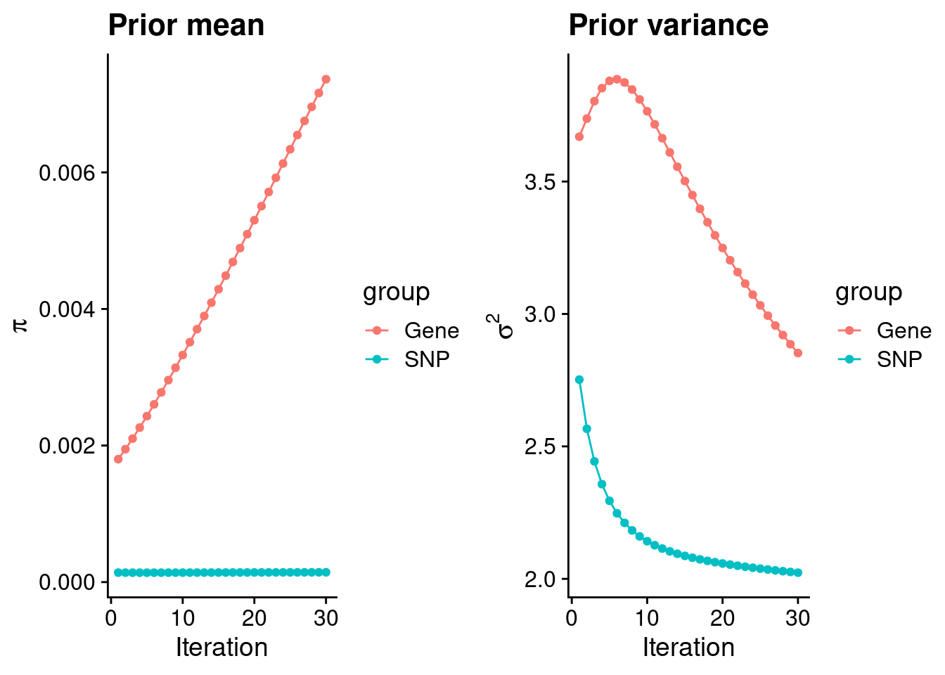
#estimated group prior
estimated_group_prior <- group_prior_rec[,ncol(group_prior_rec)]
names(estimated_group_prior) <- c("gene", "snp")
estimated_group_prior["snp"] <- estimated_group_prior["snp"]*thin #adjust parameter to account for thin argument
print(estimated_group_prior)
gene snp
0.0073643182 0.0001430957 #estimated group prior variance
estimated_group_prior_var <- group_prior_var_rec[,ncol(group_prior_var_rec)]
names(estimated_group_prior_var) <- c("gene", "snp")
print(estimated_group_prior_var) gene snp
2.852495 2.023209 #report sample size
print(sample_size)[1] 108706#report group size
group_size <- c(nrow(ctwas_gene_res), n_snps)
print(group_size)[1] 11095 8697330#estimated group PVE
estimated_group_pve <- estimated_group_prior_var*estimated_group_prior*group_size/sample_size #check PVE calculation
names(estimated_group_pve) <- c("gene", "snp")
print(estimated_group_pve) gene snp
0.002144032 0.023163273 #compare sum(PIP*mu2/sample_size) with above PVE calculation
c(sum(ctwas_gene_res$PVE),sum(ctwas_snp_res$PVE))[1] 0.02479924 0.37804101Genes with highest PIPs
#distribution of PIPs
hist(ctwas_gene_res$susie_pip, xlim=c(0,1), main="Distribution of Gene PIPs")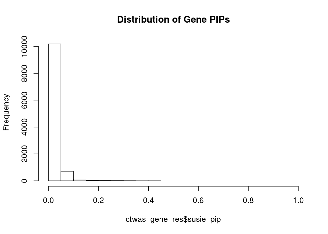
#genes with PIP>0.8 or 20 highest PIPs
head(ctwas_gene_res[order(-ctwas_gene_res$susie_pip),report_cols], max(sum(ctwas_gene_res$susie_pip>0.8), 20))
genename region_tag susie_pip mu2 PVE z
2237 TBL2 7_47 0.428 29.69 1.2e-04 3.99
7786 CATSPER2 15_16 0.381 28.52 1.0e-04 4.04
10436 STMN3 20_38 0.347 28.53 9.1e-05 4.54
8243 LIMS1 2_65 0.342 26.09 8.2e-05 3.74
7700 CCT2 12_43 0.330 28.21 8.6e-05 -4.44
6686 HIST1H2BD 6_20 0.305 24.54 6.9e-05 3.63
893 ARHGAP15 2_85 0.303 24.11 6.7e-05 3.32
1800 N4BP1 16_26 0.300 24.41 6.7e-05 3.34
2966 PCGF1 2_48 0.282 24.41 6.3e-05 3.30
4890 CDK9 9_66 0.277 23.90 6.1e-05 3.23
3226 SLC5A9 1_30 0.268 24.53 6.1e-05 -3.39
10908 SAP25 7_61 0.266 22.92 5.6e-05 -3.11
5300 CDAN1 15_16 0.256 25.08 5.9e-05 3.53
5083 MYOF 10_59 0.255 23.64 5.5e-05 -3.24
2011 CCDC61 19_32 0.253 24.81 5.8e-05 3.29
5205 PIANP 12_7 0.252 23.73 5.5e-05 3.27
7350 EXO5 1_25 0.237 23.08 5.0e-05 -3.33
5837 ATG12 5_69 0.232 22.98 4.9e-05 3.09
730 ATP1B3 3_87 0.222 22.15 4.5e-05 -3.23
9760 NELFA 4_3 0.221 22.27 4.5e-05 3.23Genes with largest effect sizes
#plot PIP vs effect size
plot(ctwas_gene_res$susie_pip, ctwas_gene_res$mu2, xlab="PIP", ylab="mu^2", main="Gene PIPs vs Effect Size")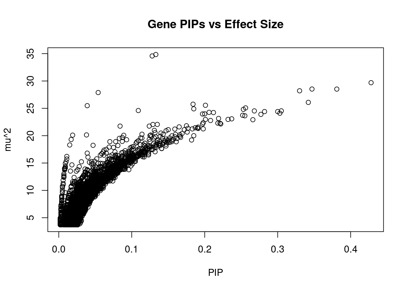
#genes with 20 largest effect sizes
head(ctwas_gene_res[order(-ctwas_gene_res$mu2),report_cols],20)
genename region_tag susie_pip mu2 PVE z
10791 RNF5 6_26 0.133 34.84 4.3e-05 3.85
10790 AGER 6_26 0.128 34.58 4.1e-05 -4.11
2237 TBL2 7_47 0.428 29.69 1.2e-04 3.99
10436 STMN3 20_38 0.347 28.53 9.1e-05 4.54
7786 CATSPER2 15_16 0.381 28.52 1.0e-04 4.04
7700 CCT2 12_43 0.330 28.21 8.6e-05 -4.44
10845 TRIM39 6_26 0.054 27.89 1.4e-05 -3.15
8243 LIMS1 2_65 0.342 26.09 8.2e-05 3.74
11602 ZNF709 19_11 0.184 25.76 4.4e-05 -3.39
1230 GRAMD1A 19_24 0.201 25.56 4.7e-05 3.28
10802 NELFE 6_26 0.039 25.49 9.2e-06 3.23
5300 CDAN1 15_16 0.256 25.08 5.9e-05 3.53
8142 LGALS9 17_18 0.185 24.91 4.3e-05 3.25
2011 CCDC61 19_32 0.253 24.81 5.8e-05 3.29
3244 ATF6 1_79 0.109 24.60 2.5e-05 3.41
6686 HIST1H2BD 6_20 0.305 24.54 6.9e-05 3.63
3226 SLC5A9 1_30 0.268 24.53 6.1e-05 -3.39
2966 PCGF1 2_48 0.282 24.41 6.3e-05 3.30
1800 N4BP1 16_26 0.300 24.41 6.7e-05 3.34
3640 USP45 6_67 0.206 24.27 4.6e-05 -3.84Genes with highest PVE
#genes with 20 highest pve
head(ctwas_gene_res[order(-ctwas_gene_res$PVE),report_cols],20)
genename region_tag susie_pip mu2 PVE z
2237 TBL2 7_47 0.428 29.69 1.2e-04 3.99
7786 CATSPER2 15_16 0.381 28.52 1.0e-04 4.04
10436 STMN3 20_38 0.347 28.53 9.1e-05 4.54
7700 CCT2 12_43 0.330 28.21 8.6e-05 -4.44
8243 LIMS1 2_65 0.342 26.09 8.2e-05 3.74
6686 HIST1H2BD 6_20 0.305 24.54 6.9e-05 3.63
893 ARHGAP15 2_85 0.303 24.11 6.7e-05 3.32
1800 N4BP1 16_26 0.300 24.41 6.7e-05 3.34
2966 PCGF1 2_48 0.282 24.41 6.3e-05 3.30
3226 SLC5A9 1_30 0.268 24.53 6.1e-05 -3.39
4890 CDK9 9_66 0.277 23.90 6.1e-05 3.23
5300 CDAN1 15_16 0.256 25.08 5.9e-05 3.53
2011 CCDC61 19_32 0.253 24.81 5.8e-05 3.29
10908 SAP25 7_61 0.266 22.92 5.6e-05 -3.11
5083 MYOF 10_59 0.255 23.64 5.5e-05 -3.24
5205 PIANP 12_7 0.252 23.73 5.5e-05 3.27
7350 EXO5 1_25 0.237 23.08 5.0e-05 -3.33
5837 ATG12 5_69 0.232 22.98 4.9e-05 3.09
5756 LRIG1 3_45 0.219 23.15 4.7e-05 3.17
6410 ABCA10 17_39 0.212 24.23 4.7e-05 -3.21Genes with largest z scores
#genes with 20 largest z scores
head(ctwas_gene_res[order(-abs(ctwas_gene_res$z)),report_cols],20)
genename region_tag susie_pip mu2 PVE z
10436 STMN3 20_38 0.347 28.53 9.1e-05 4.54
7700 CCT2 12_43 0.330 28.21 8.6e-05 -4.44
10790 AGER 6_26 0.128 34.58 4.1e-05 -4.11
7786 CATSPER2 15_16 0.381 28.52 1.0e-04 4.04
2237 TBL2 7_47 0.428 29.69 1.2e-04 3.99
10381 ZGPAT 20_38 0.109 19.07 1.9e-05 3.87
10791 RNF5 6_26 0.133 34.84 4.3e-05 3.85
3640 USP45 6_67 0.206 24.27 4.6e-05 -3.84
8243 LIMS1 2_65 0.342 26.09 8.2e-05 3.74
6686 HIST1H2BD 6_20 0.305 24.54 6.9e-05 3.63
10669 SFT2D1 6_108 0.191 21.57 3.8e-05 3.55
5300 CDAN1 15_16 0.256 25.08 5.9e-05 3.53
3244 ATF6 1_79 0.109 24.60 2.5e-05 3.41
3226 SLC5A9 1_30 0.268 24.53 6.1e-05 -3.39
11602 ZNF709 19_11 0.184 25.76 4.4e-05 -3.39
2462 NDUFC1 4_92 0.208 22.78 4.4e-05 3.38
8537 ORMDL3 17_23 0.176 20.66 3.4e-05 3.37
7554 WBSCR27 7_47 0.165 21.61 3.3e-05 -3.36
1626 PAPLN 14_34 0.093 19.26 1.6e-05 -3.36
831 GSDMB 17_23 0.166 20.18 3.1e-05 3.36Comparing z scores and PIPs
#set nominal signifiance threshold for z scores
alpha <- 0.05

#bonferroni adjusted threshold for z scores
sig_thresh <- qnorm(1-(alpha/nrow(ctwas_gene_res)/2), lower=T)

#Q-Q plot for z scores
obs_z <- ctwas_gene_res$z[order(ctwas_gene_res$z)]
exp_z <- qnorm((1:nrow(ctwas_gene_res))/nrow(ctwas_gene_res))

plot(exp_z, obs_z, xlab="Expected z", ylab="Observed z", main="Gene z score Q-Q plot")
abline(a=0,b=1)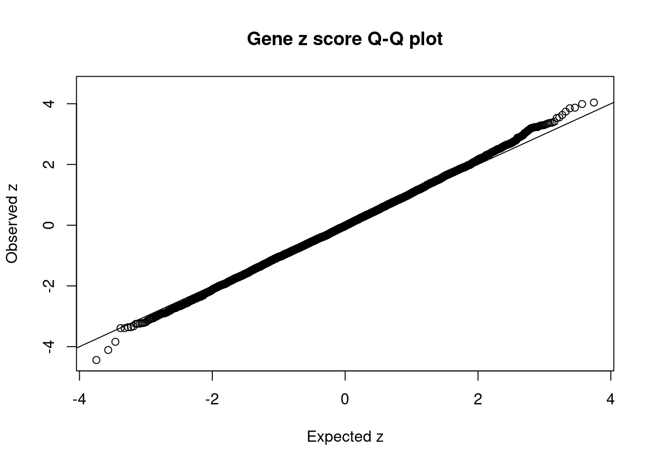
| Version | Author | Date |
|---|---|---|
| dfd2b5f | wesleycrouse | 2021-09-07 |
#plot z score vs PIP
plot(abs(ctwas_gene_res$z), ctwas_gene_res$susie_pip, xlab="abs(z)", ylab="PIP")
abline(v=sig_thresh, col="red", lty=2)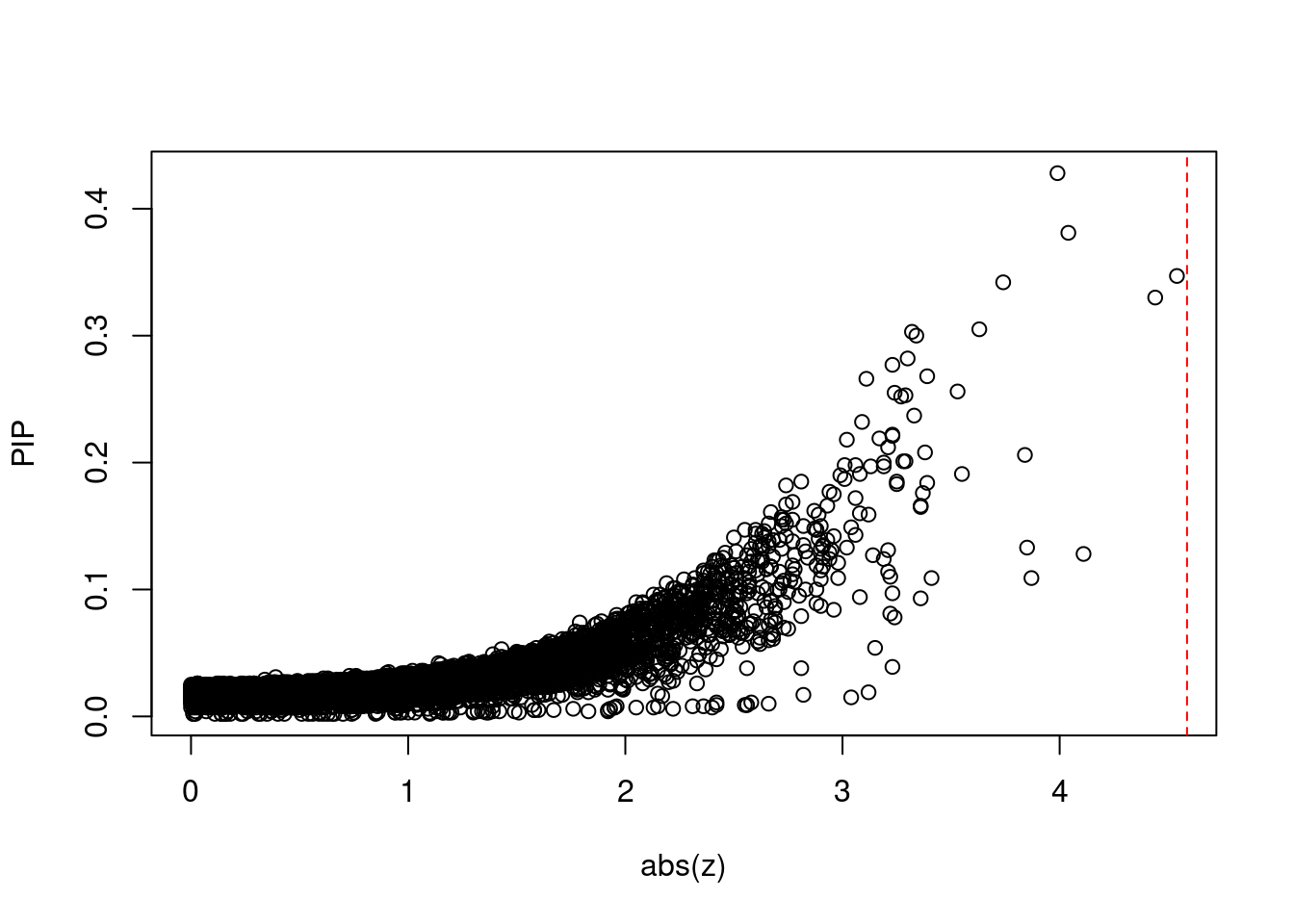
| Version | Author | Date |
|---|---|---|
| dfd2b5f | wesleycrouse | 2021-09-07 |
#proportion of significant z scores
mean(abs(ctwas_gene_res$z) > sig_thresh)
[1] 0#genes with most significant z scores
head(ctwas_gene_res[order(-abs(ctwas_gene_res$z)),report_cols],20) genename region_tag susie_pip mu2 PVE z
10436 STMN3 20_38 0.347 28.53 9.1e-05 4.54
7700 CCT2 12_43 0.330 28.21 8.6e-05 -4.44
10790 AGER 6_26 0.128 34.58 4.1e-05 -4.11
7786 CATSPER2 15_16 0.381 28.52 1.0e-04 4.04
2237 TBL2 7_47 0.428 29.69 1.2e-04 3.99
10381 ZGPAT 20_38 0.109 19.07 1.9e-05 3.87
10791 RNF5 6_26 0.133 34.84 4.3e-05 3.85
3640 USP45 6_67 0.206 24.27 4.6e-05 -3.84
8243 LIMS1 2_65 0.342 26.09 8.2e-05 3.74
6686 HIST1H2BD 6_20 0.305 24.54 6.9e-05 3.63
10669 SFT2D1 6_108 0.191 21.57 3.8e-05 3.55
5300 CDAN1 15_16 0.256 25.08 5.9e-05 3.53
3244 ATF6 1_79 0.109 24.60 2.5e-05 3.41
3226 SLC5A9 1_30 0.268 24.53 6.1e-05 -3.39
11602 ZNF709 19_11 0.184 25.76 4.4e-05 -3.39
2462 NDUFC1 4_92 0.208 22.78 4.4e-05 3.38
8537 ORMDL3 17_23 0.176 20.66 3.4e-05 3.37
7554 WBSCR27 7_47 0.165 21.61 3.3e-05 -3.36
1626 PAPLN 14_34 0.093 19.26 1.6e-05 -3.36
831 GSDMB 17_23 0.166 20.18 3.1e-05 3.36Locus plots for genes and SNPs
ctwas_gene_res_sortz <- ctwas_gene_res[order(-abs(ctwas_gene_res$z)),]

n_plots <- 5
for (region_tag_plot in head(unique(ctwas_gene_res_sortz$region_tag), n_plots)){
  ctwas_res_region <-  ctwas_res[ctwas_res$region_tag==region_tag_plot,]
  start <- min(ctwas_res_region$pos)
  end <- max(ctwas_res_region$pos)

  ctwas_res_region <- ctwas_res_region[order(ctwas_res_region$pos),]
  ctwas_res_region_gene <- ctwas_res_region[ctwas_res_region$type=="gene",]
  ctwas_res_region_snp <- ctwas_res_region[ctwas_res_region$type=="SNP",]

  #region name
  print(paste0("Region: ", region_tag_plot))

  #table of genes in region
  print(ctwas_res_region_gene[,report_cols])

  par(mfrow=c(4,1))

  #gene z scores
  plot(ctwas_res_region_gene$pos, abs(ctwas_res_region_gene$z), xlab="Position", ylab="abs(gene_z)", xlim=c(start,end),
   ylim=c(0,max(sig_thresh, abs(ctwas_res_region_gene$z))),
   main=paste0("Region: ", region_tag_plot))
  abline(h=sig_thresh,col="red",lty=2)

  #significance threshold for SNPs
  alpha_snp <- 5*10^(-8)
  sig_thresh_snp <- qnorm(1-alpha_snp/2, lower=T)

  #snp z scores
  plot(ctwas_res_region_snp$pos, abs(ctwas_res_region_snp$z), xlab="Position", ylab="abs(snp_z)",xlim=c(start,end),
   ylim=c(0,max(sig_thresh_snp, max(abs(ctwas_res_region_snp$z)))))
  abline(h=sig_thresh_snp,col="purple",lty=2)

  #gene pips
  plot(ctwas_res_region_gene$pos, ctwas_res_region_gene$susie_pip, xlab="Position", ylab="Gene PIP", xlim=c(start,end), ylim=c(0,1))
  abline(h=0.8,col="blue",lty=2)

  #snp pips
  plot(ctwas_res_region_snp$pos, ctwas_res_region_snp$susie_pip, xlab="Position", ylab="SNP PIP", xlim=c(start,end), ylim=c(0,1))
  abline(h=0.8,col="blue",lty=2)
}
[1] "Region: 20_38"
genename region_tag susie_pip mu2 PVE z
1694 GMEB2 20_38 0.026 8.24 2.0e-06 -2.33
11906 RTEL1 20_38 0.014 3.71 4.9e-07 0.80
10436 STMN3 20_38 0.347 28.53 9.1e-05 4.54
10381 ZGPAT 20_38 0.109 19.07 1.9e-05 3.87
11612 TNFRSF6B 20_38 0.016 4.73 7.1e-07 -0.89
1699 ARFRP1 20_38 0.078 16.48 1.2e-05 -3.24
10746 LIME1 20_38 0.015 3.91 5.3e-07 0.71
3805 SLC2A4RG 20_38 0.015 4.13 5.7e-07 -0.11
10575 UCKL1 20_38 0.132 20.56 2.5e-05 -2.90
10318 ZNF512B 20_38 0.018 5.43 8.9e-07 -0.98
4203 SAMD10 20_38 0.051 13.26 6.2e-06 2.12
1677 PRPF6 20_38 0.031 9.47 2.7e-06 1.70
10268 LINC00176 20_38 0.014 3.83 5.1e-07 -0.16
10745 SOX18 20_38 0.037 10.82 3.7e-06 1.73
8489 RGS19 20_38 0.017 5.00 7.8e-07 -0.69
3804 OPRL1 20_38 0.018 5.56 9.3e-07 -0.80
8488 LKAAEAR1 20_38 0.015 4.12 5.7e-07 -0.32
10744 PCMTD2 20_38 0.044 12.10 4.9e-06 1.98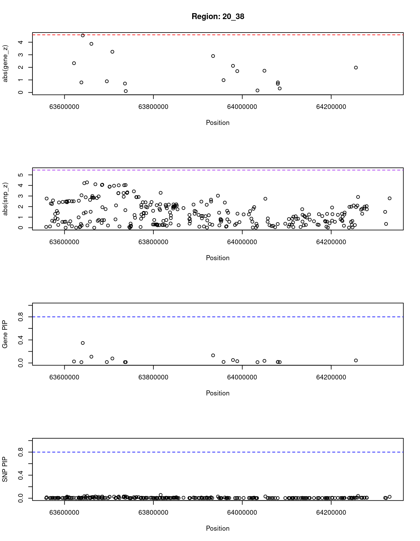
| Version | Author | Date |
|---|---|---|
| dfd2b5f | wesleycrouse | 2021-09-07 |
[1] "Region: 12_43"
       genename region_tag susie_pip   mu2     PVE     z
7699       FRS2      12_43     0.022  7.19 1.5e-06 -1.50
7700       CCT2      12_43     0.330 28.21 8.6e-05 -4.44
3944     RAB3IP      12_43     0.015  4.36 6.1e-07 -0.30
11892 LINC01481      12_43     0.014  3.77 4.9e-07  0.03
2635      CNOT2      12_43     0.016  4.71 6.9e-07 -0.63
4746     KCNMB4      12_43     0.070 15.77 1.0e-05 -2.44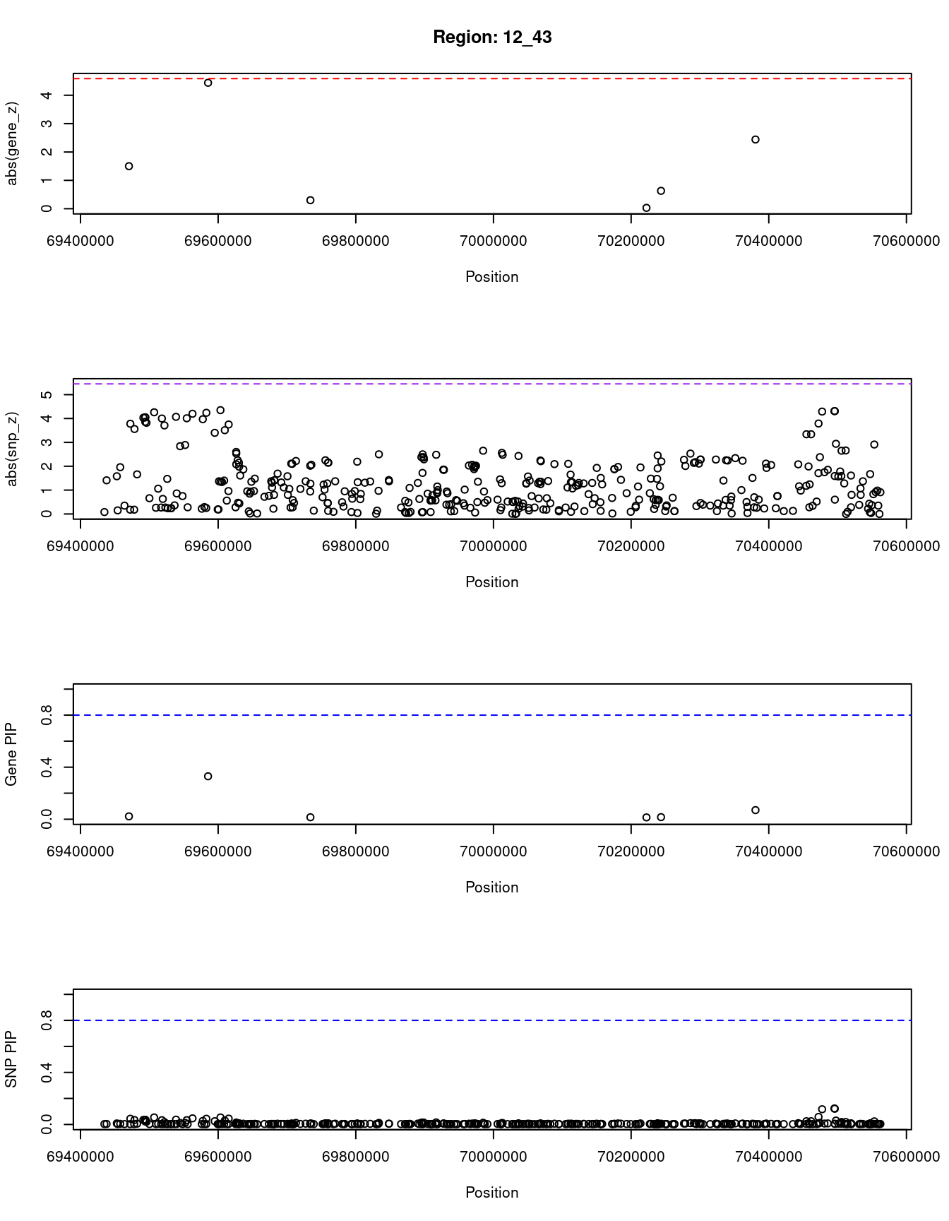
| Version | Author | Date |
|---|---|---|
| dfd2b5f | wesleycrouse | 2021-09-07 |
[1] "Region: 6_26"
               genename region_tag susie_pip   mu2     PVE     z
10855             HLA-G       6_26     0.005  9.71 4.2e-07  1.58
12599             HCP5B       6_26     0.004  7.77 2.6e-07 -1.35
10968             HLA-A       6_26     0.004  7.63 2.5e-07  1.30
10853              HCG9       6_26     0.003  5.43 1.3e-07  0.86
10851           PPP1R11       6_26     0.005 10.07 4.6e-07 -1.60
661               ZNRD1       6_26     0.003  6.36 1.8e-07  0.97
10850             RNF39       6_26     0.003  5.96 1.6e-07 -0.94
10848            TRIM10       6_26     0.007 12.47 7.8e-07  1.95
10847            TRIM15       6_26     0.004  8.04 2.8e-07  1.32
11418            TRIM26       6_26     0.003  5.06 1.2e-07 -0.75
10845            TRIM39       6_26     0.054 27.89 1.4e-05 -3.15
11563             RPP21       6_26     0.003  6.30 1.7e-07  1.03
10844             HLA-E       6_26     0.003  7.00 2.1e-07 -1.20
10841           MRPS18B       6_26     0.002  3.74 7.2e-08 -0.14
10840          C6orf136       6_26     0.007 13.01 8.8e-07 -1.95
10839             DHX16       6_26     0.002  4.45 9.5e-08  0.59
5868            PPP1R18       6_26     0.005  9.65 4.1e-07 -1.58
4976                NRM       6_26     0.005 10.74 5.3e-07  1.67
4970              FLOT1       6_26     0.003  6.01 1.6e-07 -0.94
10230              TUBB       6_26     0.002  4.39 9.3e-08 -0.51
4971               IER3       6_26     0.004  8.84 3.4e-07 -1.42
11120         LINC00243       6_26     0.004  8.24 2.9e-07 -1.34
10843              DDR1       6_26     0.002  4.72 1.0e-07  0.85
11052            GTF2H4       6_26     0.002  3.73 7.2e-08  0.02
4978              VARS2       6_26     0.002  3.86 7.6e-08  0.32
10838            CCHCR1       6_26     0.004  8.99 3.5e-07 -1.39
4969              TCF19       6_26     0.004  8.79 3.4e-07  1.92
10966             HCG27       6_26     0.002  4.67 1.0e-07  1.10
10837            POU5F1       6_26     0.006 11.27 6.0e-07  1.76
10836             HLA-C       6_26     0.003  7.31 2.3e-07 -1.30
10788            NOTCH4       6_26     0.019 20.10 3.5e-06  3.12
11439             HLA-B       6_26     0.002  4.19 8.6e-08  0.74
12270 XXbac-BPG181B23.7       6_26     0.003  5.85 1.5e-07 -1.51
10834              MICA       6_26     0.004  8.14 2.9e-07 -1.83
10833              MICB       6_26     0.003  6.71 1.9e-07  0.96
10830              LST1       6_26     0.004  8.62 3.2e-07  1.49
10619            DDX39B       6_26     0.002  3.77 7.3e-08  0.24
11050          ATP6V1G2       6_26     0.002  4.18 8.6e-08 -0.16
10831           NFKBIL1       6_26     0.002  3.78 7.4e-08 -0.18
11282               LTA       6_26     0.002  3.87 7.6e-08 -0.35
11296               LTB       6_26     0.002  3.95 7.9e-08 -0.40
11395               TNF       6_26     0.002  4.68 1.0e-07 -0.56
10829              NCR3       6_26     0.003  6.50 1.8e-07 -1.37
10828              AIF1       6_26     0.002  3.71 7.2e-08 -0.14
10827            PRRC2A       6_26     0.003  6.64 1.9e-07  1.36
10826              BAG6       6_26     0.002  3.98 8.0e-08  0.23
10825              APOM       6_26     0.006 11.04 5.7e-07  2.22
10824           C6orf47       6_26     0.002  4.49 9.6e-08 -0.54
10822            CSNK2B       6_26     0.002  4.96 1.1e-07  0.61
10823            GPANK1       6_26     0.003  5.23 1.2e-07 -0.59
11539            LY6G5B       6_26     0.017 19.30 3.0e-06 -2.82
10821            LY6G5C       6_26     0.007 12.39 7.7e-07 -2.13
11639            LY6G6D       6_26     0.008 13.73 1.0e-06 -2.31
10818            MPIG6B       6_26     0.002  4.90 1.1e-07  0.65
10819            LY6G6C       6_26     0.011 15.73 1.5e-06 -2.42
11048             DDAH2       6_26     0.008 14.02 1.1e-06 -2.15
10817              MSH5       6_26     0.006 11.87 6.9e-07 -1.93
11047             CLIC1       6_26     0.007 12.74 8.3e-07  2.40
11327            SAPCD1       6_26     0.002  4.53 9.8e-08 -0.70
10814              VWA7       6_26     0.002  3.71 7.1e-08  0.01
10809           C6orf48       6_26     0.007 12.52 7.9e-07 -2.05
10813              VARS       6_26     0.004  7.53 2.4e-07  1.13
10812              LSM2       6_26     0.008 13.89 1.1e-06 -1.96
10811            HSPA1L       6_26     0.002  4.48 9.6e-08  0.63
10808              NEU1       6_26     0.009 14.35 1.2e-06  2.56
10807           SLC44A4       6_26     0.008 14.03 1.1e-06 -2.36
7712                 C2       6_26     0.009 14.35 1.2e-06 -2.56
10805             EHMT2       6_26     0.003  6.55 1.9e-07 -1.10
10802             NELFE       6_26     0.039 25.49 9.2e-06  3.23
10801            SKIV2L       6_26     0.003  6.55 1.9e-07 -1.18
10797             STK19       6_26     0.003  7.11 2.2e-07  1.16
10800               DXO       6_26     0.003  6.48 1.8e-07 -1.16
11652               C4A       6_26     0.010 15.25 1.4e-06  2.66
11218               C4B       6_26     0.009 14.10 1.1e-06 -2.55
11374           CYP21A2       6_26     0.002  3.99 8.0e-08 -0.66
11193              PPT2       6_26     0.003  5.53 1.4e-07  0.85
11043             ATF6B       6_26     0.003  5.65 1.4e-07  1.00
10795             FKBPL       6_26     0.002  3.71 7.2e-08  0.01
10794             PRRT1       6_26     0.011 16.21 1.7e-06 -2.58
10791              RNF5       6_26     0.133 34.84 4.3e-05  3.85
11565             EGFL8       6_26     0.005 10.56 5.1e-07  1.92
10792            AGPAT1       6_26     0.009 14.90 1.3e-06  2.42
10790              AGER       6_26     0.128 34.58 4.1e-05 -4.11
10789              PBX2       6_26     0.015 18.30 2.5e-06  3.04
10608          HLA-DRB5       6_26     0.003  7.03 2.1e-07 -1.19
10325          HLA-DQA1       6_26     0.002  3.72 7.2e-08  0.16
11490          HLA-DQA2       6_26     0.002  4.01 8.0e-08  0.43
11389          HLA-DQB2       6_26     0.002  3.71 7.2e-08 -0.11
9260           HLA-DQB1       6_26     0.002  3.75 7.3e-08  0.31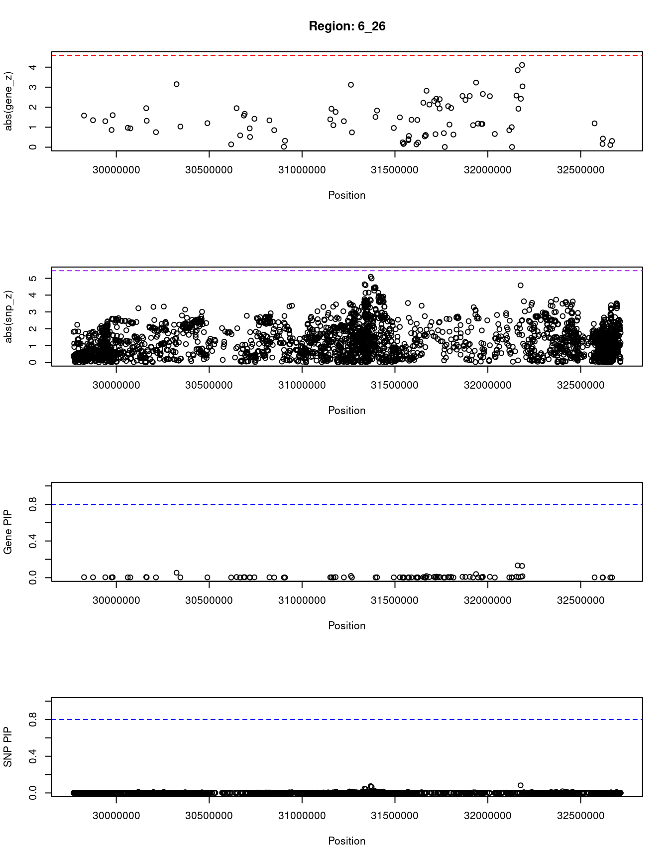
| Version | Author | Date |
|---|---|---|
| dfd2b5f | wesleycrouse | 2021-09-07 |
[1] "Region: 15_16"
     genename region_tag susie_pip   mu2     PVE     z
1325   SNAP23      15_16     0.039 10.46 3.8e-06  1.85
9382   LRRC57      15_16     0.048 11.96 5.3e-06  2.02
5030    HAUS2      15_16     0.068 14.58 9.1e-06  2.46
6785   STARD9      15_16     0.017  4.08 6.3e-07  0.28
5300    CDAN1      15_16     0.256 25.08 5.9e-05  3.53
4064    TTBK2      15_16     0.019  5.16 9.2e-07 -0.97
7829  CCNDBP1      15_16     0.024  6.91 1.5e-06  1.24
1905     TGM5      15_16     0.016  3.72 5.4e-07  0.29
8115     ADAL      15_16     0.019  4.91 8.4e-07  0.23
8116    LCMT2      15_16     0.019  4.91 8.4e-07  0.23
5034  TUBGCP4      15_16     0.020  5.36 9.8e-07 -0.83
5295  ZSCAN29      15_16     0.017  4.01 6.1e-07 -0.51
7831    MAP1A      15_16     0.018  4.53 7.4e-07  0.91
7786 CATSPER2      15_16     0.381 28.52 1.0e-04  4.04
7839    PDIA3      15_16     0.020  5.59 1.1e-06 -1.02
4065     ELL3      15_16     0.019  4.88 8.3e-07 -0.67
5294    SERF2      15_16     0.019  4.88 8.3e-07 -0.67
5291    MFAP1      15_16     0.017  4.10 6.3e-07  0.90
1323    WDR76      15_16     0.016  3.75 5.5e-07 -0.19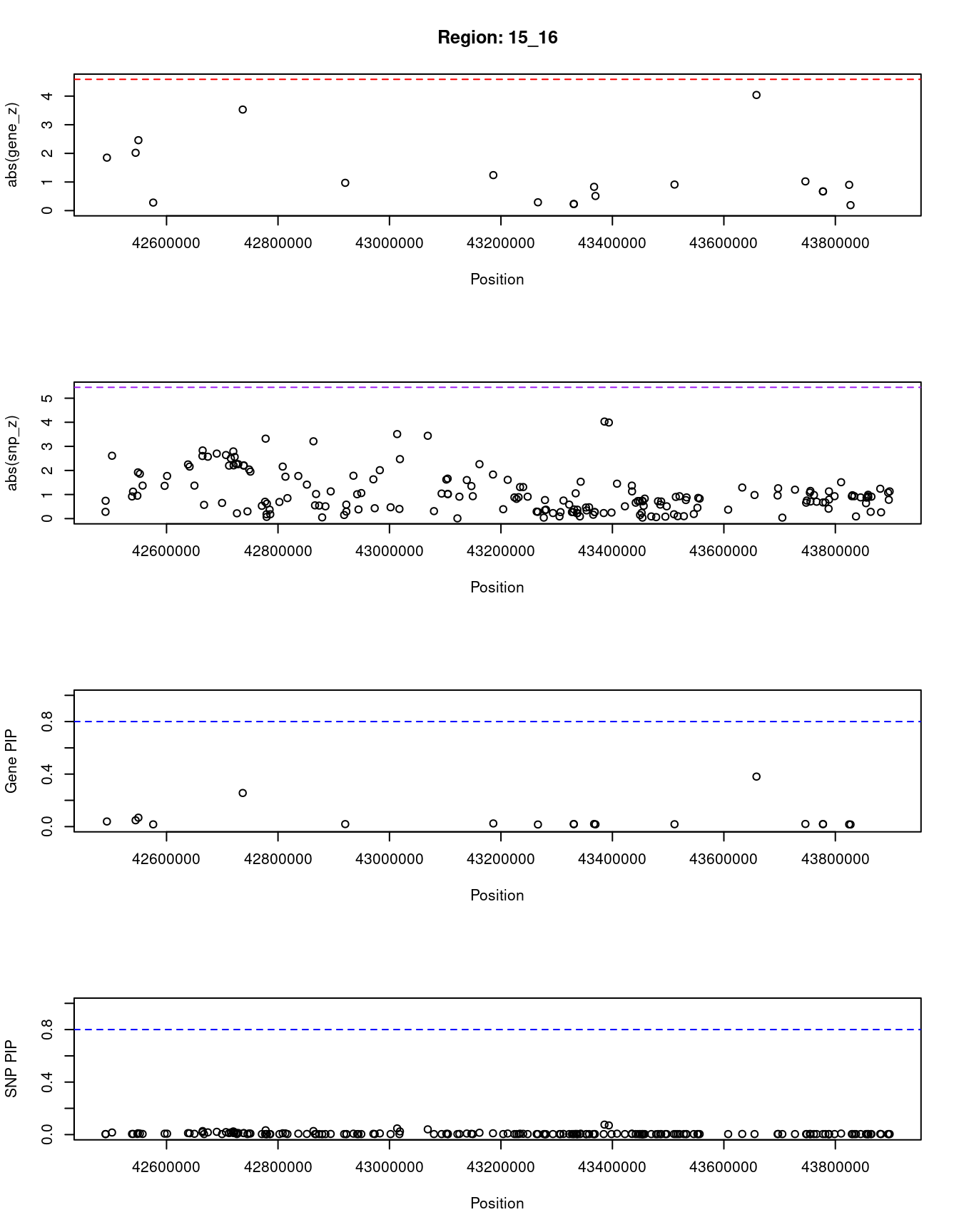
| Version | Author | Date |
|---|---|---|
| dfd2b5f | wesleycrouse | 2021-09-07 |
[1] "Region: 7_47"
      genename region_tag susie_pip   mu2     PVE     z
10243   POM121       7_47     0.019  5.16 9.0e-07 -0.89
4172     NSUN5       7_47     0.017  4.17 6.4e-07 -0.33
165      BAZ1B       7_47     0.025  7.22 1.7e-06 -1.24
2237      TBL2       7_47     0.428 29.69 1.2e-04  3.99
8997    VPS37D       7_47     0.016  3.89 5.8e-07  0.37
778    WBSCR22       7_47     0.017  4.41 7.0e-07 -0.61
8995   DNAJC30       7_47     0.017  4.44 7.1e-07 -0.63
2172    ABHD11       7_47     0.023  6.49 1.4e-06  1.59
2175     STX1A       7_47     0.023  6.63 1.4e-06  1.62
10175    CLDN4       7_47     0.124 19.34 2.2e-05  3.19
7554   WBSCR27       7_47     0.165 21.61 3.3e-05 -3.36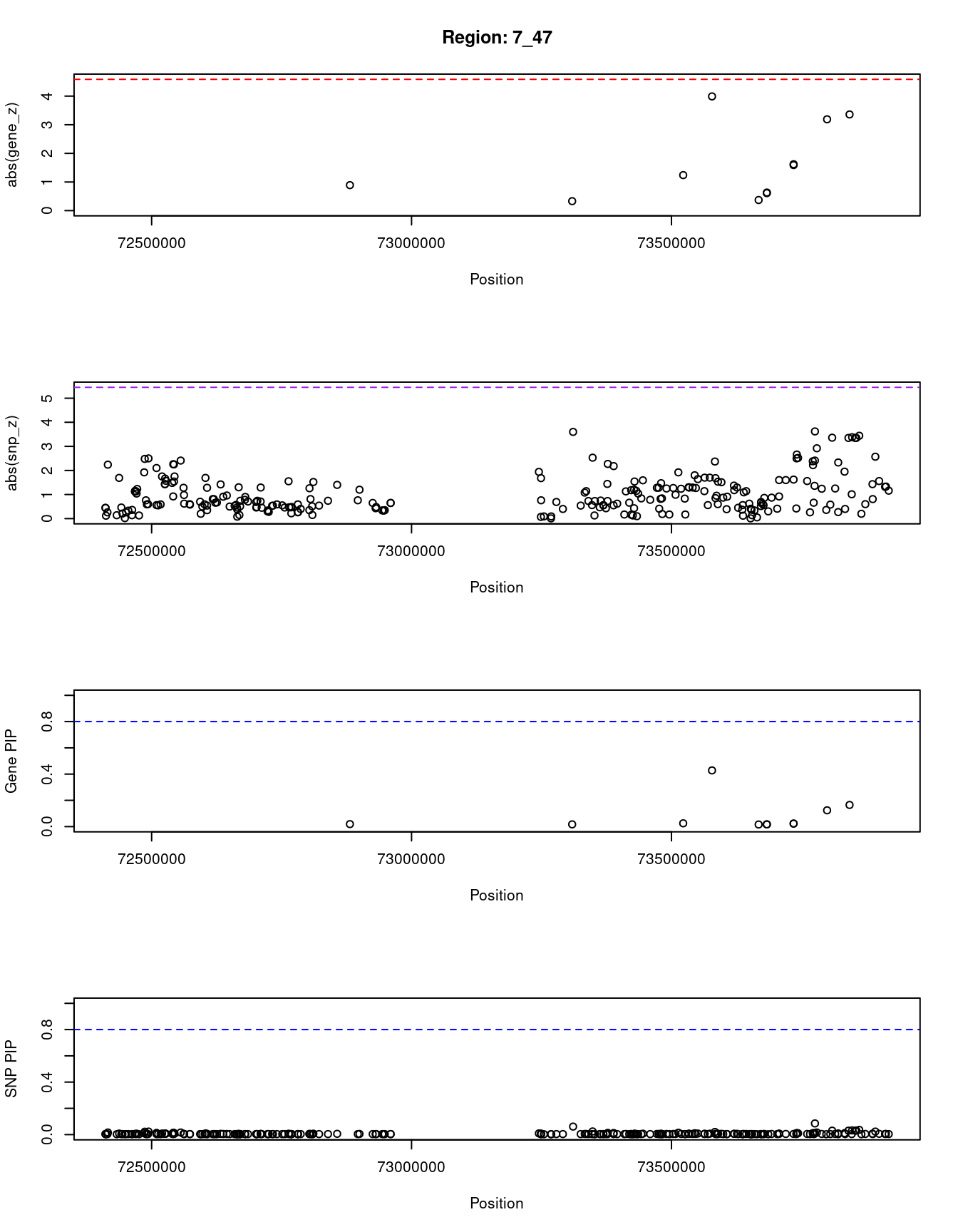
| Version | Author | Date |
|---|---|---|
| dfd2b5f | wesleycrouse | 2021-09-07 |
SNPs with highest PIPs
#snps with PIP>0.8 or 20 highest PIPs
head(ctwas_snp_res[order(-ctwas_snp_res$susie_pip),report_cols_snps],
max(sum(ctwas_snp_res$susie_pip>0.8), 20))
id region_tag susie_pip mu2 PVE z
265377 rs4109437 4_122 1.000 60.00 5.5e-04 9.52
524158 rs17343073 10_14 0.942 57.55 5.0e-04 9.45
72021 rs17432480 2_9 0.625 27.25 1.6e-04 -4.80
13754 rs7543243 1_29 0.540 28.49 1.4e-04 5.12
250242 rs6857487 4_96 0.378 35.21 1.2e-04 4.86
526099 rs551737161 10_16 0.320 35.43 1.0e-04 -3.38
235650 rs1508422 4_67 0.307 33.60 9.5e-05 -4.63
319239 rs116004855 5_104 0.290 32.92 8.8e-05 4.29
160246 rs774067422 3_42 0.289 32.09 8.5e-05 4.46
838797 rs8117150 20_27 0.265 31.60 7.7e-05 4.12
100467 rs1898846 2_66 0.255 33.64 7.9e-05 -4.76
460516 rs16907708 8_57 0.251 32.32 7.5e-05 -4.22
231831 rs60955950 4_60 0.243 31.94 7.2e-05 -4.35
24492 rs59104377 1_51 0.240 31.07 6.9e-05 -4.09
467073 rs138854257 8_70 0.239 31.27 6.9e-05 4.14
744211 rs12927956 16_27 0.236 32.08 7.0e-05 4.12
52803 rs600396 1_105 0.230 30.71 6.5e-05 4.06
739370 rs35419776 16_17 0.230 31.13 6.6e-05 -4.05
549774 rs11189853 10_63 0.228 30.96 6.5e-05 3.99
412256 rs6958957 7_56 0.225 30.65 6.4e-05 4.00SNPs with largest effect sizes
#plot PIP vs effect size
plot(ctwas_snp_res$susie_pip, ctwas_snp_res$mu2, xlab="PIP", ylab="mu^2", main="SNP PIPs vs Effect Size")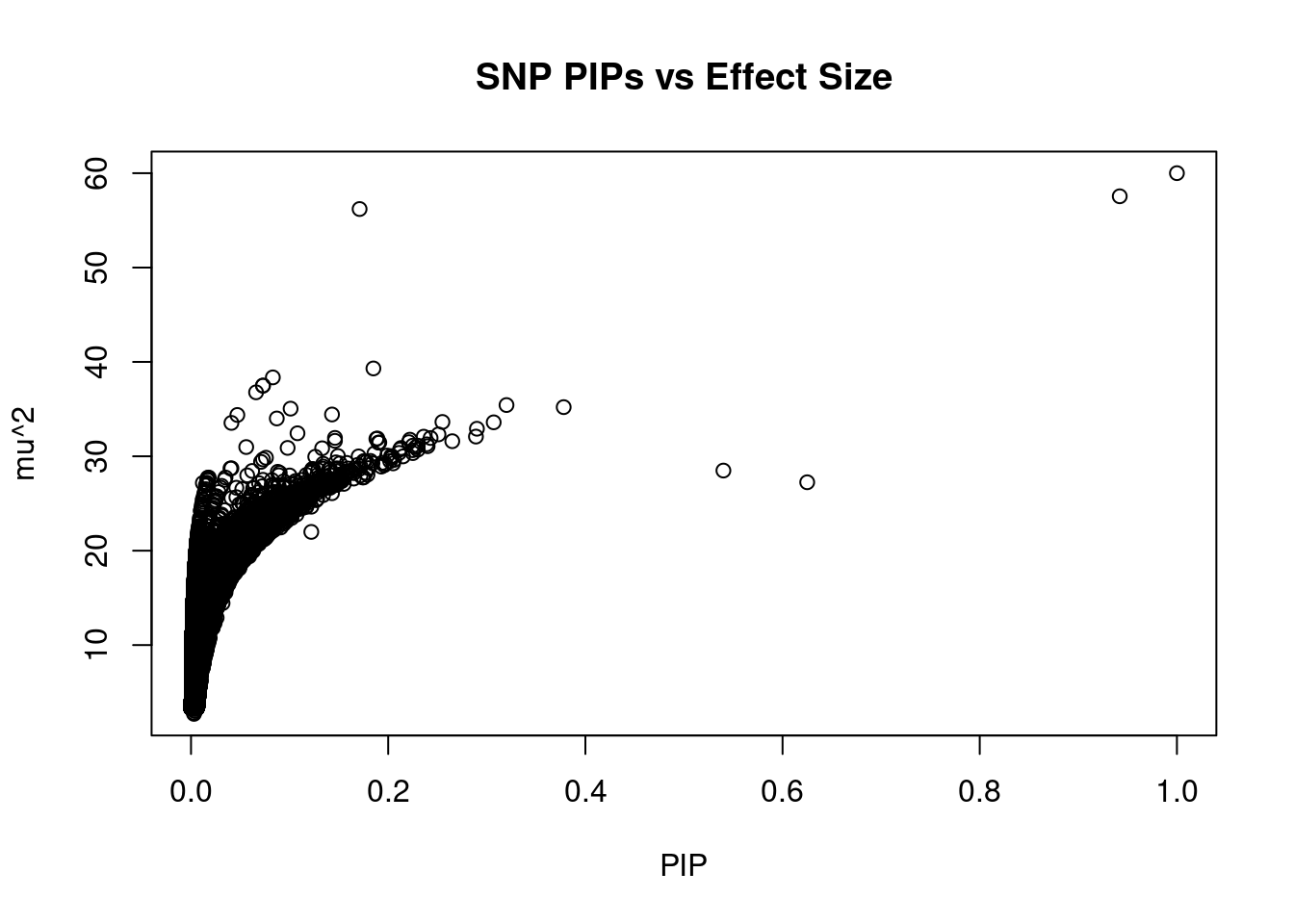
| Version | Author | Date |
|---|---|---|
| dfd2b5f | wesleycrouse | 2021-09-07 |
#SNPs with 50 largest effect sizes
head(ctwas_snp_res[order(-ctwas_snp_res$mu2),report_cols_snps],50)
id region_tag susie_pip mu2 PVE z
265377 rs4109437 4_122 1.000 60.00 5.5e-04 9.52
524158 rs17343073 10_14 0.942 57.55 5.0e-04 9.45
524165 rs113795872 10_14 0.171 56.20 8.9e-05 9.02
228055 rs13146163 4_52 0.185 39.31 6.7e-05 -5.05
334929 rs16869385 6_26 0.083 38.36 2.9e-05 4.58
334505 rs13215664 6_26 0.073 37.50 2.5e-05 5.09
334506 rs4991645 6_26 0.073 37.48 2.5e-05 5.09
334512 rs2395492 6_26 0.066 36.78 2.2e-05 4.99
526099 rs551737161 10_16 0.320 35.43 1.0e-04 -3.38
250242 rs6857487 4_96 0.378 35.21 1.2e-04 4.86
228335 rs2194125 4_52 0.101 35.05 3.3e-05 -4.10
828978 rs1987579 20_5 0.143 34.43 4.5e-05 4.11
334338 rs34548997 6_26 0.047 34.38 1.5e-05 4.64
228067 rs147760951 4_52 0.087 34.01 2.7e-05 -4.08
100467 rs1898846 2_66 0.255 33.64 7.9e-05 -4.76
235650 rs1508422 4_67 0.307 33.60 9.5e-05 -4.63
334373 rs6929132 6_26 0.041 33.54 1.3e-05 4.59
319239 rs116004855 5_104 0.290 32.92 8.8e-05 4.29
828796 rs6038431 20_5 0.108 32.44 3.2e-05 4.23
460516 rs16907708 8_57 0.251 32.32 7.5e-05 -4.22
160246 rs774067422 3_42 0.289 32.09 8.5e-05 4.46
744211 rs12927956 16_27 0.236 32.08 7.0e-05 4.12
519225 rs10795199 10_7 0.146 31.95 4.3e-05 4.02
231831 rs60955950 4_60 0.243 31.94 7.2e-05 -4.35
522764 rs7090451 10_12 0.189 31.89 5.5e-05 -4.38
522762 rs6602637 10_12 0.188 31.85 5.5e-05 -4.38
570432 rs118142338 11_17 0.222 31.76 6.5e-05 -4.03
786058 rs1160103 18_9 0.146 31.64 4.2e-05 4.10
838797 rs8117150 20_27 0.265 31.60 7.7e-05 4.12
279316 rs13179493 5_26 0.221 31.50 6.4e-05 -4.60
13745 rs2065944 1_29 0.191 31.46 5.5e-05 4.53
100473 rs4848374 2_66 0.190 31.45 5.5e-05 -4.62
467073 rs138854257 8_70 0.239 31.27 6.9e-05 4.14
739370 rs35419776 16_17 0.230 31.13 6.6e-05 -4.05
788005 rs138729533 18_12 0.225 31.13 6.5e-05 4.07
24492 rs59104377 1_51 0.240 31.07 6.9e-05 -4.09
227616 rs6836560 4_52 0.056 30.98 1.6e-05 -3.72
549774 rs11189853 10_63 0.228 30.96 6.5e-05 3.99
94783 rs17022590 2_54 0.098 30.89 2.8e-05 -3.88
853043 rs73352324 21_15 0.213 30.88 6.0e-05 -4.33
796375 rs1443568 18_28 0.133 30.85 3.8e-05 4.07
534353 rs116858637 10_33 0.212 30.72 6.0e-05 -3.95
52803 rs600396 1_105 0.230 30.71 6.5e-05 4.06
412256 rs6958957 7_56 0.225 30.65 6.4e-05 4.00
662569 rs79125844 13_32 0.211 30.36 5.9e-05 4.21
848984 rs191739247 21_7 0.225 30.34 6.3e-05 3.93
713324 rs8033332 15_15 0.186 30.30 5.2e-05 -4.65
499269 rs1175334 9_39 0.199 30.08 5.5e-05 -4.27
155840 rs73065135 3_33 0.149 30.03 4.1e-05 4.67
819757 rs146928263 19_27 0.203 30.02 5.6e-05 -3.93SNPs with highest PVE
#SNPs with 50 highest pve
head(ctwas_snp_res[order(-ctwas_snp_res$PVE),report_cols_snps],50)
id region_tag susie_pip mu2 PVE z
265377 rs4109437 4_122 1.000 60.00 5.5e-04 9.52
524158 rs17343073 10_14 0.942 57.55 5.0e-04 9.45
72021 rs17432480 2_9 0.625 27.25 1.6e-04 -4.80
13754 rs7543243 1_29 0.540 28.49 1.4e-04 5.12
250242 rs6857487 4_96 0.378 35.21 1.2e-04 4.86
526099 rs551737161 10_16 0.320 35.43 1.0e-04 -3.38
235650 rs1508422 4_67 0.307 33.60 9.5e-05 -4.63
524165 rs113795872 10_14 0.171 56.20 8.9e-05 9.02
319239 rs116004855 5_104 0.290 32.92 8.8e-05 4.29
160246 rs774067422 3_42 0.289 32.09 8.5e-05 4.46
100467 rs1898846 2_66 0.255 33.64 7.9e-05 -4.76
838797 rs8117150 20_27 0.265 31.60 7.7e-05 4.12
460516 rs16907708 8_57 0.251 32.32 7.5e-05 -4.22
231831 rs60955950 4_60 0.243 31.94 7.2e-05 -4.35
744211 rs12927956 16_27 0.236 32.08 7.0e-05 4.12
24492 rs59104377 1_51 0.240 31.07 6.9e-05 -4.09
467073 rs138854257 8_70 0.239 31.27 6.9e-05 4.14
228055 rs13146163 4_52 0.185 39.31 6.7e-05 -5.05
739370 rs35419776 16_17 0.230 31.13 6.6e-05 -4.05
52803 rs600396 1_105 0.230 30.71 6.5e-05 4.06
549774 rs11189853 10_63 0.228 30.96 6.5e-05 3.99
570432 rs118142338 11_17 0.222 31.76 6.5e-05 -4.03
788005 rs138729533 18_12 0.225 31.13 6.5e-05 4.07
279316 rs13179493 5_26 0.221 31.50 6.4e-05 -4.60
412256 rs6958957 7_56 0.225 30.65 6.4e-05 4.00
848984 rs191739247 21_7 0.225 30.34 6.3e-05 3.93
534353 rs116858637 10_33 0.212 30.72 6.0e-05 -3.95
853043 rs73352324 21_15 0.213 30.88 6.0e-05 -4.33
290066 rs7716273 5_46 0.215 29.99 5.9e-05 -4.16
662569 rs79125844 13_32 0.211 30.36 5.9e-05 4.21
56561 rs552055532 1_111 0.203 29.79 5.6e-05 -3.85
313386 rs186927917 5_91 0.206 29.62 5.6e-05 3.82
792180 rs12458728 18_21 0.204 29.97 5.6e-05 -3.94
819757 rs146928263 19_27 0.203 30.02 5.6e-05 -3.93
13745 rs2065944 1_29 0.191 31.46 5.5e-05 4.53
100473 rs4848374 2_66 0.190 31.45 5.5e-05 -4.62
499269 rs1175334 9_39 0.199 30.08 5.5e-05 -4.27
522762 rs6602637 10_12 0.188 31.85 5.5e-05 -4.38
522764 rs7090451 10_12 0.189 31.89 5.5e-05 -4.38
530237 rs79262861 10_25 0.205 29.25 5.5e-05 -3.89
811724 rs199991194 19_12 0.202 29.49 5.5e-05 3.85
179917 rs112861149 3_80 0.197 29.21 5.3e-05 3.91
267915 rs77497829 5_5 0.196 29.06 5.2e-05 3.79
551652 rs10509810 10_67 0.194 29.32 5.2e-05 -4.02
713324 rs8033332 15_15 0.186 30.30 5.2e-05 -4.65
619672 rs117751804 12_29 0.193 28.91 5.1e-05 -3.92
655852 rs79782223 13_17 0.184 29.27 5.0e-05 3.82
133887 rs79567528 2_133 0.182 29.51 4.9e-05 -4.29
81889 rs9284745 2_27 0.180 28.75 4.8e-05 -3.78
89602 rs562157001 2_44 0.176 29.48 4.8e-05 3.80SNPs with largest z scores
#SNPs with 50 largest z scores
head(ctwas_snp_res[order(-abs(ctwas_snp_res$z)),report_cols_snps],50)
id region_tag susie_pip mu2 PVE z
265377 rs4109437 4_122 1.000 60.00 5.5e-04 9.52
524158 rs17343073 10_14 0.942 57.55 5.0e-04 9.45
524165 rs113795872 10_14 0.171 56.20 8.9e-05 9.02
524169 rs3858184 10_14 0.012 27.17 2.9e-06 6.34
13754 rs7543243 1_29 0.540 28.49 1.4e-04 5.12
334505 rs13215664 6_26 0.073 37.50 2.5e-05 5.09
334506 rs4991645 6_26 0.073 37.48 2.5e-05 5.09
228055 rs13146163 4_52 0.185 39.31 6.7e-05 -5.05
334512 rs2395492 6_26 0.066 36.78 2.2e-05 4.99
565641 rs61889814 11_8 0.134 29.21 3.6e-05 4.99
565639 rs59090117 11_8 0.124 28.64 3.3e-05 4.96
565637 rs55879783 11_8 0.123 28.59 3.2e-05 4.95
250242 rs6857487 4_96 0.378 35.21 1.2e-04 4.86
72021 rs17432480 2_9 0.625 27.25 1.6e-04 -4.80
100467 rs1898846 2_66 0.255 33.64 7.9e-05 -4.76
155840 rs73065135 3_33 0.149 30.03 4.1e-05 4.67
713324 rs8033332 15_15 0.186 30.30 5.2e-05 -4.65
334338 rs34548997 6_26 0.047 34.38 1.5e-05 4.64
235650 rs1508422 4_67 0.307 33.60 9.5e-05 -4.63
100473 rs4848374 2_66 0.190 31.45 5.5e-05 -4.62
279316 rs13179493 5_26 0.221 31.50 6.4e-05 -4.60
334373 rs6929132 6_26 0.041 33.54 1.3e-05 4.59
334929 rs16869385 6_26 0.083 38.36 2.9e-05 4.58
13745 rs2065944 1_29 0.191 31.46 5.5e-05 4.53
13757 rs6681140 1_29 0.122 21.99 2.5e-05 4.53
334562 rs542630771 6_26 0.017 27.73 4.5e-06 4.47
542391 rs7909516 10_49 0.172 28.93 4.6e-05 4.47
740076 rs35830321 16_19 0.156 28.06 4.0e-05 -4.47
160246 rs774067422 3_42 0.289 32.09 8.5e-05 4.46
334559 rs7752021 6_26 0.017 27.63 4.4e-06 4.46
334561 rs75098758 6_26 0.017 27.62 4.4e-06 4.46
334558 rs7771971 6_26 0.017 27.53 4.3e-06 4.45
334565 rs67484745 6_26 0.017 27.49 4.3e-06 4.45
334566 rs150737002 6_26 0.017 27.55 4.3e-06 4.45
155842 rs6768845 3_33 0.095 26.85 2.3e-05 4.44
542389 rs4531409 10_49 0.162 28.48 4.2e-05 4.44
334546 rs73398308 6_26 0.016 27.21 4.0e-06 4.43
334537 rs28623422 6_26 0.016 27.01 3.9e-06 4.42
334544 rs13437094 6_26 0.016 27.01 3.9e-06 4.42
713327 rs7183231 15_15 0.117 27.00 2.9e-05 4.42
713351 rs28810086 15_15 0.130 27.77 3.3e-05 4.42
193145 rs9865575 3_105 0.137 27.85 3.5e-05 4.41
334567 rs66862067 6_26 0.015 26.90 3.8e-06 4.41
379190 rs34430737 6_108 0.157 28.20 4.1e-05 4.40
471489 rs55781186 8_79 0.171 28.67 4.5e-05 4.39
522762 rs6602637 10_12 0.188 31.85 5.5e-05 -4.38
522764 rs7090451 10_12 0.189 31.89 5.5e-05 -4.38
193147 rs73171228 3_105 0.127 27.32 3.2e-05 4.37
542390 rs765918 10_49 0.141 27.49 3.6e-05 4.37
193148 rs6808176 3_105 0.126 27.25 3.2e-05 4.36Gene set enrichment for genes with PIP>0.8
#GO enrichment analysis
library(enrichR)
Welcome to enrichR
Checking connection ... Enrichr ... Connection is Live!
FlyEnrichr ... Connection is available!
WormEnrichr ... Connection is available!
YeastEnrichr ... Connection is available!
FishEnrichr ... Connection is available!dbs <- c("GO_Biological_Process_2021", "GO_Cellular_Component_2021", "GO_Molecular_Function_2021")
genes <- ctwas_gene_res$genename[ctwas_gene_res$susie_pip>0.8]
#number of genes for gene set enrichment
length(genes)[1] 0if (length(genes)>0){
GO_enrichment <- enrichr(genes, dbs)
for (db in dbs){
print(db)
df <- GO_enrichment[[db]]
df <- df[df$Adjusted.P.value<0.05,c("Term", "Overlap", "Adjusted.P.value", "Genes")]
print(df)
}
#DisGeNET enrichment
# devtools::install_bitbucket("ibi_group/disgenet2r")
library(disgenet2r)
disgenet_api_key <- get_disgenet_api_key(
email = "wesleycrouse@gmail.com",
password = "uchicago1" )
Sys.setenv(DISGENET_API_KEY= disgenet_api_key)
res_enrich <-disease_enrichment(entities=genes, vocabulary = "HGNC",
database = "CURATED" )
df <- res_enrich@qresult[1:10, c("Description", "FDR", "Ratio", "BgRatio")]
print(df)
#WebGestalt enrichment
library(WebGestaltR)
background <- ctwas_gene_res$genename
#listGeneSet()
databases <- c("pathway_KEGG", "disease_GLAD4U", "disease_OMIM")
enrichResult <- WebGestaltR(enrichMethod="ORA", organism="hsapiens",
interestGene=genes, referenceGene=background,
enrichDatabase=databases, interestGeneType="genesymbol",
referenceGeneType="genesymbol", isOutput=F)
print(enrichResult[,c("description", "size", "overlap", "FDR", "database", "userId")])
}
sessionInfo()R version 3.6.1 (2019-07-05)
Platform: x86_64-pc-linux-gnu (64-bit)
Running under: Scientific Linux 7.4 (Nitrogen)
Matrix products: default
BLAS/LAPACK: /software/openblas-0.2.19-el7-x86_64/lib/libopenblas_haswellp-r0.2.19.so
locale:
[1] LC_CTYPE=en_US.UTF-8 LC_NUMERIC=C
[3] LC_TIME=en_US.UTF-8 LC_COLLATE=en_US.UTF-8
[5] LC_MONETARY=en_US.UTF-8 LC_MESSAGES=en_US.UTF-8
[7] LC_PAPER=en_US.UTF-8 LC_NAME=C
[9] LC_ADDRESS=C LC_TELEPHONE=C
[11] LC_MEASUREMENT=en_US.UTF-8 LC_IDENTIFICATION=C
attached base packages:
[1] stats graphics grDevices utils datasets methods base
other attached packages:
[1] enrichR_3.0 cowplot_1.0.0 ggplot2_3.3.3
loaded via a namespace (and not attached):
[1] Biobase_2.44.0 httr_1.4.1
[3] bit64_4.0.5 assertthat_0.2.1
[5] stats4_3.6.1 blob_1.2.1
[7] BSgenome_1.52.0 GenomeInfoDbData_1.2.1
[9] Rsamtools_2.0.0 yaml_2.2.0
[11] progress_1.2.2 pillar_1.6.1
[13] RSQLite_2.2.7 lattice_0.20-38
[15] glue_1.4.2 digest_0.6.20
[17] GenomicRanges_1.36.0 promises_1.0.1
[19] XVector_0.24.0 colorspace_1.4-1
[21] htmltools_0.3.6 httpuv_1.5.1
[23] Matrix_1.2-18 XML_3.98-1.20
[25] pkgconfig_2.0.3 biomaRt_2.40.1
[27] zlibbioc_1.30.0 purrr_0.3.4
[29] scales_1.1.0 whisker_0.3-2
[31] later_0.8.0 BiocParallel_1.18.0
[33] git2r_0.26.1 tibble_3.1.2
[35] farver_2.1.0 generics_0.0.2
[37] IRanges_2.18.1 ellipsis_0.3.2
[39] withr_2.4.1 cachem_1.0.5
[41] SummarizedExperiment_1.14.1 GenomicFeatures_1.36.3
[43] BiocGenerics_0.30.0 magrittr_2.0.1
[45] crayon_1.4.1 memoise_2.0.0
[47] evaluate_0.14 fs_1.3.1
[49] fansi_0.5.0 tools_3.6.1
[51] data.table_1.14.0 prettyunits_1.0.2
[53] hms_1.1.0 lifecycle_1.0.0
[55] matrixStats_0.57.0 stringr_1.4.0
[57] S4Vectors_0.22.1 munsell_0.5.0
[59] DelayedArray_0.10.0 AnnotationDbi_1.46.0
[61] Biostrings_2.52.0 compiler_3.6.1
[63] GenomeInfoDb_1.20.0 rlang_0.4.11
[65] grid_3.6.1 RCurl_1.98-1.1
[67] rjson_0.2.20 VariantAnnotation_1.30.1
[69] labeling_0.3 bitops_1.0-6
[71] rmarkdown_1.13 gtable_0.3.0
[73] curl_3.3 DBI_1.1.1
[75] R6_2.5.0 GenomicAlignments_1.20.1
[77] dplyr_1.0.7 knitr_1.23
[79] rtracklayer_1.44.0 utf8_1.2.1
[81] fastmap_1.1.0 bit_4.0.4
[83] workflowr_1.6.2 rprojroot_2.0.2
[85] stringi_1.4.3 parallel_3.6.1
[87] Rcpp_1.0.6 vctrs_0.3.8
[89] tidyselect_1.1.0 xfun_0.8