Microalbumin in urine - Liver
wesleycrouse
2021-09-09
Last updated: 2021-09-09
Checks: 6 1
Knit directory: ctwas_applied/
This reproducible R Markdown analysis was created with workflowr (version 1.6.2). The Checks tab describes the reproducibility checks that were applied when the results were created. The Past versions tab lists the development history.
The R Markdown file has unstaged changes. To know which version of the R Markdown file created these results, you’ll want to first commit it to the Git repo. If you’re still working on the analysis, you can ignore this warning. When you’re finished, you can run wflow_publish to commit the R Markdown file and build the HTML.
Great job! The global environment was empty. Objects defined in the global environment can affect the analysis in your R Markdown file in unknown ways. For reproduciblity it’s best to always run the code in an empty environment.
The command set.seed(20210726) was run prior to running the code in the R Markdown file. Setting a seed ensures that any results that rely on randomness, e.g. subsampling or permutations, are reproducible.
Great job! Recording the operating system, R version, and package versions is critical for reproducibility.
Nice! There were no cached chunks for this analysis, so you can be confident that you successfully produced the results during this run.
Great job! Using relative paths to the files within your workflowr project makes it easier to run your code on other machines.
Great! You are using Git for version control. Tracking code development and connecting the code version to the results is critical for reproducibility.
The results in this page were generated with repository version 59e5f4d. See the Past versions tab to see a history of the changes made to the R Markdown and HTML files.
Note that you need to be careful to ensure that all relevant files for the analysis have been committed to Git prior to generating the results (you can use wflow_publish or wflow_git_commit). workflowr only checks the R Markdown file, but you know if there are other scripts or data files that it depends on. Below is the status of the Git repository when the results were generated:
Unstaged changes:
    Modified:   analysis/ukb-d-30500_irnt_Liver.Rmd
Note that any generated files, e.g. HTML, png, CSS, etc., are not included in this status report because it is ok for generated content to have uncommitted changes.
These are the previous versions of the repository in which changes were made to the R Markdown (analysis/ukb-d-30500_irnt_Liver.Rmd) and HTML (docs/ukb-d-30500_irnt_Liver.html) files. If you’ve configured a remote Git repository (see ?wflow_git_remote), click on the hyperlinks in the table below to view the files as they were in that past version.
| File | Version | Author | Date | Message |
|---|---|---|---|---|
| Rmd | cbf7408 | wesleycrouse | 2021-09-08 | adding enrichment to reports |
| html | cbf7408 | wesleycrouse | 2021-09-08 | adding enrichment to reports |
| Rmd | 4970e3e | wesleycrouse | 2021-09-08 | updating reports |
| html | 4970e3e | wesleycrouse | 2021-09-08 | updating reports |
| Rmd | 627a4e1 | wesleycrouse | 2021-09-07 | adding heritability |
| Rmd | dfd2b5f | wesleycrouse | 2021-09-07 | regenerating reports |
| html | dfd2b5f | wesleycrouse | 2021-09-07 | regenerating reports |
| Rmd | 61b53b3 | wesleycrouse | 2021-09-06 | updated PVE calculation |
| html | 61b53b3 | wesleycrouse | 2021-09-06 | updated PVE calculation |
| Rmd | 837dd01 | wesleycrouse | 2021-09-01 | adding additional fixedsigma report |
| Rmd | d0a5417 | wesleycrouse | 2021-08-30 | adding new reports to the index |
| Rmd | 0922de7 | wesleycrouse | 2021-08-18 | updating all reports with locus plots |
| html | 0922de7 | wesleycrouse | 2021-08-18 | updating all reports with locus plots |
| html | 1c62980 | wesleycrouse | 2021-08-11 | Updating reports |
| Rmd | 5981e80 | wesleycrouse | 2021-08-11 | Adding more reports |
| html | 5981e80 | wesleycrouse | 2021-08-11 | Adding more reports |
| Rmd | 05a98b7 | wesleycrouse | 2021-08-07 | adding additional results |
| html | 05a98b7 | wesleycrouse | 2021-08-07 | adding additional results |
| html | 03e541c | wesleycrouse | 2021-07-29 | Cleaning up report generation |
| html | 276893d | wesleycrouse | 2021-07-29 | Updating reports |
| html | 4068e9b | wesleycrouse | 2021-07-29 | finalizing automation |
| Rmd | 0e62fa9 | wesleycrouse | 2021-07-29 | Automating reports |
| html | 0e62fa9 | wesleycrouse | 2021-07-29 | Automating reports |
Overview
These are the results of a ctwas analysis of the UK Biobank trait Microalbumin in urine using Liver gene weights.
The GWAS was conducted by the Neale Lab, and the biomarker traits we analyzed are discussed here. Summary statistics were obtained from IEU OpenGWAS using GWAS ID: ukb-d-30500_irnt. Results were obtained from from IEU rather than Neale Lab because they are in a standardard format (GWAS VCF). Note that 3 of the 34 biomarker traits were not available from IEU and were excluded from analysis.
The weights are mashr GTEx v8 models on Liver eQTL obtained from PredictDB. We performed a full harmonization of the variants, including recovering strand ambiguous variants. This procedure is discussed in a separate document. (TO-DO: add report that describes harmonization)
LD matrices were computed from a 10% subset of Neale lab subjects. Subjects were matched using the plate and well information from genotyping. We included only biallelic variants with MAF>0.01 in the original Neale Lab GWAS. (TO-DO: add more details [number of subjects, variants, etc])
Weight QC
TO-DO: add enhanced QC reporting (total number of weights, why each variant was missing for all genes)
qclist_all <- list()

qc_files <- paste0(results_dir, "/", list.files(results_dir, pattern="exprqc.Rd"))

for (i in 1:length(qc_files)){
  load(qc_files[i])
  chr <- unlist(strsplit(rev(unlist(strsplit(qc_files[i], "_")))[1], "[.]"))[1]
  qclist_all[[chr]] <- cbind(do.call(rbind, lapply(qclist,unlist)), as.numeric(substring(chr,4)))
}

qclist_all <- data.frame(do.call(rbind, qclist_all))
colnames(qclist_all)[ncol(qclist_all)] <- "chr"

rm(qclist, wgtlist, z_gene_chr)

#number of imputed weights
nrow(qclist_all)
[1] 10901#number of imputed weights by chromosome
table(qclist_all$chr)
   1    2    3    4    5    6    7    8    9   10   11   12   13   14   15
1070  768  652  417  494  611  548  408  405  434  634  629  195  365  354
  16   17   18   19   20   21   22
 526  663  160  859  306  114  289
#proportion of imputed weights without missing variants
mean(qclist_all$nmiss==0)[1] 0.8366205Load ctwas results
#load ctwas results
ctwas_res <- data.table::fread(paste0(results_dir, "/", analysis_id, "_ctwas.susieIrss.txt"))

#make unique identifier for regions
ctwas_res$region_tag <- paste(ctwas_res$region_tag1, ctwas_res$region_tag2, sep="_")

#compute PVE for each gene/SNP
ctwas_res$PVE = ctwas_res$susie_pip*ctwas_res$mu2/sample_size #check PVE calculation

#separate gene and SNP results
ctwas_gene_res <- ctwas_res[ctwas_res$type == "gene", ]
ctwas_gene_res <- data.frame(ctwas_gene_res)
ctwas_snp_res <- ctwas_res[ctwas_res$type == "SNP", ]
ctwas_snp_res <- data.frame(ctwas_snp_res)

#add gene information to results
sqlite <- RSQLite::dbDriver("SQLite")
db = RSQLite::dbConnect(sqlite, paste0("/project2/compbio/predictdb/mashr_models/mashr_", weight, ".db"))
query <- function(...) RSQLite::dbGetQuery(db, ...)
gene_info <- query("select gene, genename from extra")
gene_info <- query("select gene, genename, gene_type from extra")
RSQLite::dbDisconnect(db)

ctwas_gene_res <- cbind(ctwas_gene_res, gene_info[sapply(ctwas_gene_res$id, match, gene_info$gene), c("genename", "gene_type")])

#add z score to results
load(paste0(results_dir, "/", analysis_id, "_expr_z_gene.Rd"))
ctwas_gene_res$z <- z_gene[ctwas_gene_res$id,]$z

#load(paste0(results_dir, "/", analysis_id, "_expr_z_snp.Rd")) #for new version, stored after harmonization
z_snp <- readRDS(paste0(results_dir, "/", trait_id, ".RDS")) #for old version, unharmonized

z_snp <- z_snp[z_snp$id %in% ctwas_snp_res$id,] #subset snps to those included in analysis, note some are duplicated, need to match which allele was used
ctwas_snp_res$z <- z_snp$z[match(ctwas_snp_res$id, z_snp$id)] #for duplicated snps, this arbitrarily uses the first allele
ctwas_snp_res$z_flag <- as.numeric(ctwas_snp_res$id %in% z_snp$id[duplicated(z_snp$id)]) #mark the unclear z scores, flag=1

#formatting and rounding for tables
ctwas_gene_res$z <- round(ctwas_gene_res$z,2)
ctwas_snp_res$z <- round(ctwas_snp_res$z,2)
ctwas_gene_res$susie_pip <- round(ctwas_gene_res$susie_pip,3)
ctwas_snp_res$susie_pip <- round(ctwas_snp_res$susie_pip,3)
ctwas_gene_res$mu2 <- round(ctwas_gene_res$mu2,2)
ctwas_snp_res$mu2 <- round(ctwas_snp_res$mu2,2)
ctwas_gene_res$PVE <- signif(ctwas_gene_res$PVE, 2)
ctwas_snp_res$PVE <- signif(ctwas_snp_res$PVE, 2)

#merge gene and snp results with added information
ctwas_gene_res$z_flag=NA
ctwas_snp_res$genename=NA
ctwas_snp_res$gene_type=NA

ctwas_res <- rbind(ctwas_gene_res,
                   ctwas_snp_res[,colnames(ctwas_gene_res)])

#store columns to report
report_cols <- colnames(ctwas_gene_res)[!(colnames(ctwas_gene_res) %in% c("type", "region_tag1", "region_tag2", "cs_index", "gene_type", "z_flag", "id", "chrom", "pos"))]
first_cols <- c("genename", "region_tag")
report_cols <- c(first_cols, report_cols[!(report_cols %in% first_cols)])

report_cols_snps <- c("id", report_cols[-1])

#get number of SNPs from s1 results; adjust for thin
ctwas_res_s1 <- data.table::fread(paste0(results_dir, "/", analysis_id, "_ctwas.s1.susieIrss.txt"))
n_snps <- sum(ctwas_res_s1$type=="SNP")/thin
rm(ctwas_res_s1)
Check convergence of parameters
library(ggplot2)
library(cowplot)
********************************************************Note: As of version 1.0.0, cowplot does not change the default ggplot2 theme anymore. To recover the previous behavior, execute:
theme_set(theme_cowplot())********************************************************load(paste0(results_dir, "/", analysis_id, "_ctwas.s2.susieIrssres.Rd"))
df <- data.frame(niter = rep(1:ncol(group_prior_rec), 2),
value = c(group_prior_rec[1,], group_prior_rec[2,]),
group = rep(c("Gene", "SNP"), each = ncol(group_prior_rec)))
df$group <- as.factor(df$group)
df$value[df$group=="SNP"] <- df$value[df$group=="SNP"]*thin #adjust parameter to account for thin argument
p_pi <- ggplot(df, aes(x=niter, y=value, group=group)) +
geom_line(aes(color=group)) +
geom_point(aes(color=group)) +
xlab("Iteration") + ylab(bquote(pi)) +
ggtitle("Prior mean") +
theme_cowplot()
df <- data.frame(niter = rep(1:ncol(group_prior_var_rec), 2),
value = c(group_prior_var_rec[1,], group_prior_var_rec[2,]),
group = rep(c("Gene", "SNP"), each = ncol(group_prior_var_rec)))
df$group <- as.factor(df$group)
p_sigma2 <- ggplot(df, aes(x=niter, y=value, group=group)) +
geom_line(aes(color=group)) +
geom_point(aes(color=group)) +
xlab("Iteration") + ylab(bquote(sigma^2)) +
ggtitle("Prior variance") +
theme_cowplot()
plot_grid(p_pi, p_sigma2)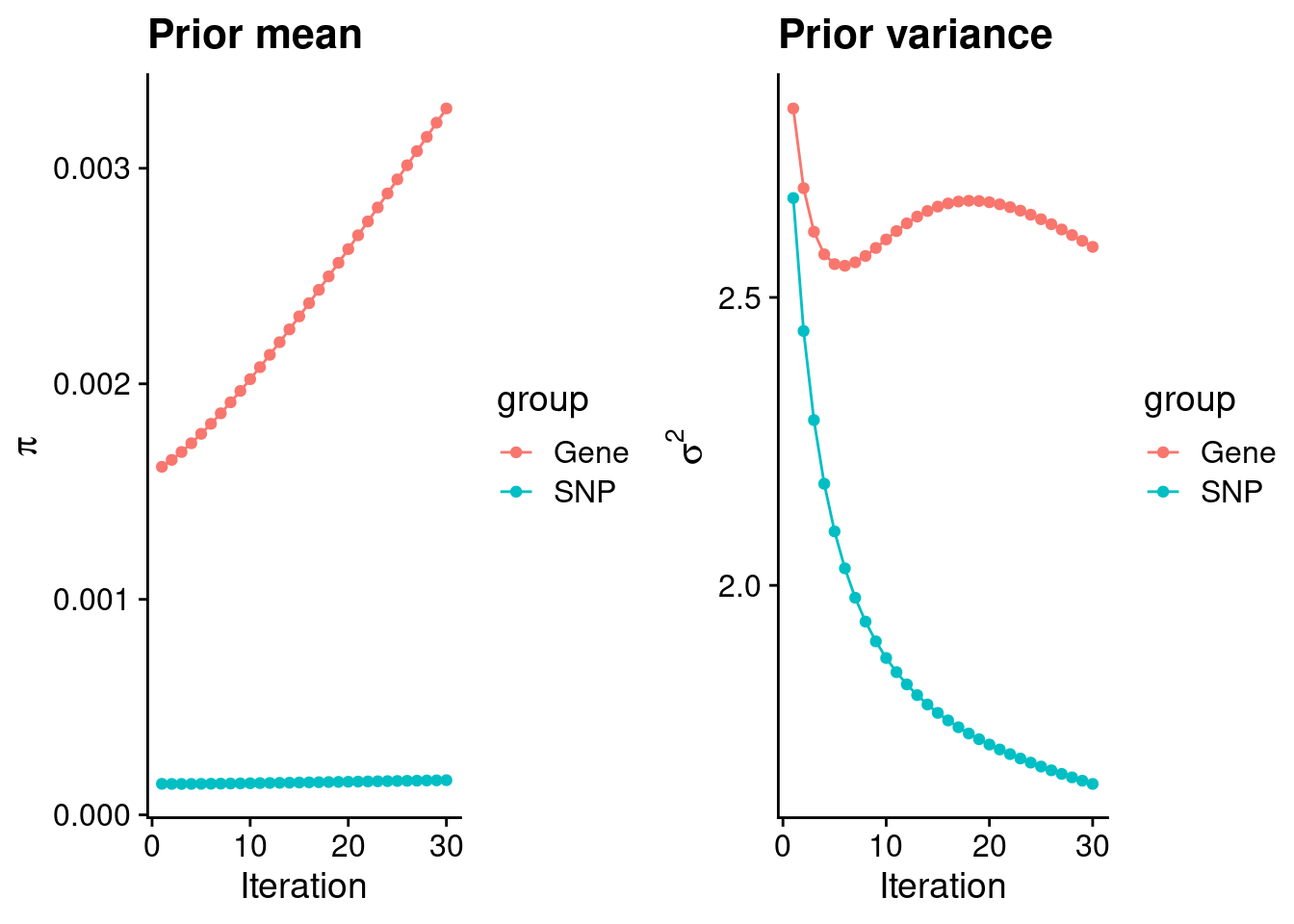
| Version | Author | Date |
|---|---|---|
| dfd2b5f | wesleycrouse | 2021-09-07 |
#estimated group prior
estimated_group_prior <- group_prior_rec[,ncol(group_prior_rec)]
names(estimated_group_prior) <- c("gene", "snp")
estimated_group_prior["snp"] <- estimated_group_prior["snp"]*thin #adjust parameter to account for thin argument
print(estimated_group_prior)
gene snp
0.0032775112 0.0001609082 #estimated group prior variance
estimated_group_prior_var <- group_prior_var_rec[,ncol(group_prior_var_rec)]
names(estimated_group_prior_var) <- c("gene", "snp")
print(estimated_group_prior_var) gene snp
2.587767 1.655200 #report sample size
print(sample_size)[1] 108706#report group size
group_size <- c(nrow(ctwas_gene_res), n_snps)
print(group_size)[1] 10901 8697330#estimated group PVE
estimated_group_pve <- estimated_group_prior_var*estimated_group_prior*group_size/sample_size #check PVE calculation
names(estimated_group_pve) <- c("gene", "snp")
print(estimated_group_pve) gene snp
0.0008505156 0.0213089004 #compare sum(PIP*mu2/sample_size) with above PVE calculation
c(sum(ctwas_gene_res$PVE),sum(ctwas_snp_res$PVE))[1] 0.01147756 0.37115625Genes with highest PIPs
#distribution of PIPs
hist(ctwas_gene_res$susie_pip, xlim=c(0,1), main="Distribution of Gene PIPs")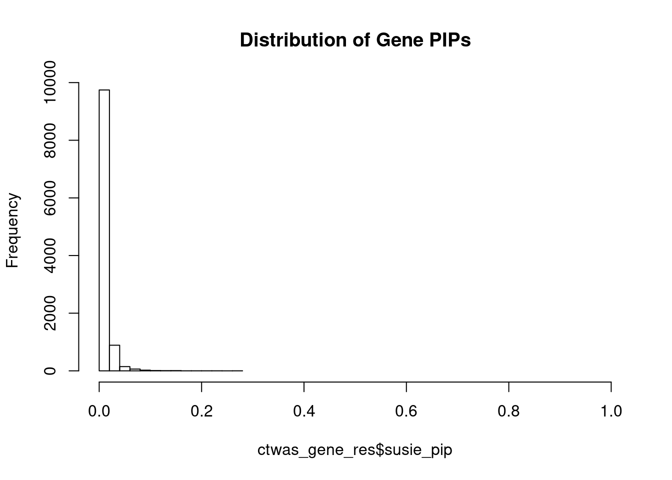
| Version | Author | Date |
|---|---|---|
| dfd2b5f | wesleycrouse | 2021-09-07 |
#genes with PIP>0.8 or 20 highest PIPs
head(ctwas_gene_res[order(-ctwas_gene_res$susie_pip),report_cols], max(sum(ctwas_gene_res$susie_pip>0.8), 20))
genename region_tag susie_pip mu2 PVE z
7656 CATSPER2 15_16 0.262 30.13 7.3e-05 4.04
8639 C12orf76 12_67 0.239 27.23 6.0e-05 -3.46
7269 TMEM184C 4_96 0.223 28.40 5.8e-05 -3.64
4061 NSUN5 7_47 0.204 27.81 5.2e-05 3.60
6602 HIST1H2BD 6_20 0.203 26.57 5.0e-05 3.63
1743 N4BP1 16_26 0.199 26.05 4.8e-05 3.34
11448 INMT 7_24 0.196 30.66 5.5e-05 3.79
4753 CDK9 9_66 0.179 25.44 4.2e-05 3.23
12272 CTC-332L22.1 5_65 0.165 26.03 3.9e-05 -3.61
5189 CDAN1 15_16 0.157 26.07 3.8e-05 3.53
10468 SFT2D1 6_108 0.156 25.07 3.6e-05 3.83
4888 CTDSPL2 15_17 0.154 25.09 3.6e-05 -3.77
3382 AKAP1 17_33 0.154 24.95 3.5e-05 3.14
7630 CLEC4E 12_8 0.150 24.57 3.4e-05 3.21
2643 CCNC 6_67 0.144 27.28 3.6e-05 3.75
5042 SHROOM3 4_52 0.143 28.05 3.7e-05 4.37
11485 ZNF709 19_10 0.143 25.51 3.4e-05 -3.39
2675 CUTA 6_28 0.140 25.68 3.3e-05 3.43
1782 NME4 16_1 0.133 24.26 3.0e-05 -3.39
1420 TOP3B 22_4 0.133 27.59 3.4e-05 3.34Genes with largest effect sizes
#plot PIP vs effect size
plot(ctwas_gene_res$susie_pip, ctwas_gene_res$mu2, xlab="PIP", ylab="mu^2", main="Gene PIPs vs Effect Size")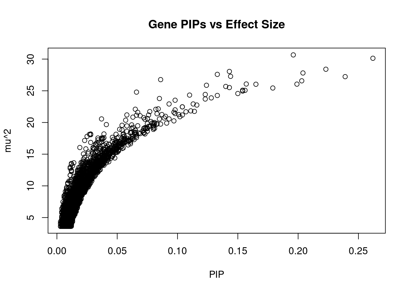
| Version | Author | Date |
|---|---|---|
| dfd2b5f | wesleycrouse | 2021-09-07 |
#genes with 20 largest effect sizes
head(ctwas_gene_res[order(-ctwas_gene_res$mu2),report_cols],20)
genename region_tag susie_pip mu2 PVE z
11448 INMT 7_24 0.196 30.66 5.5e-05 3.79
7656 CATSPER2 15_16 0.262 30.13 7.3e-05 4.04
7269 TMEM184C 4_96 0.223 28.40 5.8e-05 -3.64
5042 SHROOM3 4_52 0.143 28.05 3.7e-05 4.37
4061 NSUN5 7_47 0.204 27.81 5.2e-05 3.60
1420 TOP3B 22_4 0.133 27.59 3.4e-05 3.34
2643 CCNC 6_67 0.144 27.28 3.6e-05 3.75
8639 C12orf76 12_67 0.239 27.23 6.0e-05 -3.46
10601 AGER 6_26 0.086 26.76 2.1e-05 -4.00
6602 HIST1H2BD 6_20 0.203 26.57 5.0e-05 3.63
5189 CDAN1 15_16 0.157 26.07 3.8e-05 3.53
1743 N4BP1 16_26 0.199 26.05 4.8e-05 3.34
12272 CTC-332L22.1 5_65 0.165 26.03 3.9e-05 -3.61
9245 SETD2 3_33 0.124 25.87 3.0e-05 -4.14
2675 CUTA 6_28 0.140 25.68 3.3e-05 3.43
11485 ZNF709 19_10 0.143 25.51 3.4e-05 -3.39
4753 CDK9 9_66 0.179 25.44 4.2e-05 3.23
4888 CTDSPL2 15_17 0.154 25.09 3.6e-05 -3.77
10468 SFT2D1 6_108 0.156 25.07 3.6e-05 3.83
3382 AKAP1 17_33 0.154 24.95 3.5e-05 3.14Genes with highest PVE
#genes with 20 highest pve
head(ctwas_gene_res[order(-ctwas_gene_res$PVE),report_cols],20)
genename region_tag susie_pip mu2 PVE z
7656 CATSPER2 15_16 0.262 30.13 7.3e-05 4.04
8639 C12orf76 12_67 0.239 27.23 6.0e-05 -3.46
7269 TMEM184C 4_96 0.223 28.40 5.8e-05 -3.64
11448 INMT 7_24 0.196 30.66 5.5e-05 3.79
4061 NSUN5 7_47 0.204 27.81 5.2e-05 3.60
6602 HIST1H2BD 6_20 0.203 26.57 5.0e-05 3.63
1743 N4BP1 16_26 0.199 26.05 4.8e-05 3.34
4753 CDK9 9_66 0.179 25.44 4.2e-05 3.23
12272 CTC-332L22.1 5_65 0.165 26.03 3.9e-05 -3.61
5189 CDAN1 15_16 0.157 26.07 3.8e-05 3.53
5042 SHROOM3 4_52 0.143 28.05 3.7e-05 4.37
2643 CCNC 6_67 0.144 27.28 3.6e-05 3.75
10468 SFT2D1 6_108 0.156 25.07 3.6e-05 3.83
4888 CTDSPL2 15_17 0.154 25.09 3.6e-05 -3.77
3382 AKAP1 17_33 0.154 24.95 3.5e-05 3.14
7630 CLEC4E 12_8 0.150 24.57 3.4e-05 3.21
11485 ZNF709 19_10 0.143 25.51 3.4e-05 -3.39
1420 TOP3B 22_4 0.133 27.59 3.4e-05 3.34
2675 CUTA 6_28 0.140 25.68 3.3e-05 3.43
9245 SETD2 3_33 0.124 25.87 3.0e-05 -4.14Genes with largest z scores
#genes with 20 largest z scores
head(ctwas_gene_res[order(-abs(ctwas_gene_res$z)),report_cols],20)
genename region_tag susie_pip mu2 PVE z
5042 SHROOM3 4_52 0.143 28.05 3.7e-05 4.37
9245 SETD2 3_33 0.124 25.87 3.0e-05 -4.14
7578 FRS2 12_43 0.110 24.32 2.5e-05 -4.05
7656 CATSPER2 15_16 0.262 30.13 7.3e-05 4.04
3715 SLC2A4RG 20_38 0.093 22.92 2.0e-05 4.02
10601 AGER 6_26 0.086 26.76 2.1e-05 -4.00
10186 ZGPAT 20_38 0.084 22.15 1.7e-05 3.97
10468 SFT2D1 6_108 0.156 25.07 3.6e-05 3.83
11448 INMT 7_24 0.196 30.66 5.5e-05 3.79
9992 FAM47E 4_52 0.065 22.09 1.3e-05 3.78
4888 CTDSPL2 15_17 0.154 25.09 3.6e-05 -3.77
2643 CCNC 6_67 0.144 27.28 3.6e-05 3.75
8970 PRSS42 3_33 0.063 20.84 1.2e-05 -3.72
1647 ARFRP1 20_38 0.058 19.46 1.0e-05 3.66
7269 TMEM184C 4_96 0.223 28.40 5.8e-05 -3.64
6602 HIST1H2BD 6_20 0.203 26.57 5.0e-05 3.63
12272 CTC-332L22.1 5_65 0.165 26.03 3.9e-05 -3.61
4061 NSUN5 7_47 0.204 27.81 5.2e-05 3.60
10629 CSNK2B 6_26 0.066 24.79 1.5e-05 3.58
593 MCM10 10_11 0.128 23.88 2.8e-05 -3.55Comparing z scores and PIPs
#set nominal signifiance threshold for z scores
alpha <- 0.05

#bonferroni adjusted threshold for z scores
sig_thresh <- qnorm(1-(alpha/nrow(ctwas_gene_res)/2), lower=T)

#Q-Q plot for z scores
obs_z <- ctwas_gene_res$z[order(ctwas_gene_res$z)]
exp_z <- qnorm((1:nrow(ctwas_gene_res))/nrow(ctwas_gene_res))

plot(exp_z, obs_z, xlab="Expected z", ylab="Observed z", main="Gene z score Q-Q plot")
abline(a=0,b=1)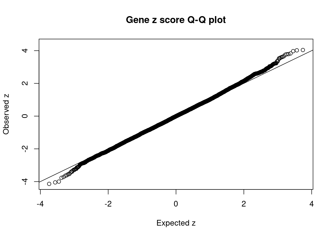
| Version | Author | Date |
|---|---|---|
| dfd2b5f | wesleycrouse | 2021-09-07 |
#plot z score vs PIP
plot(abs(ctwas_gene_res$z), ctwas_gene_res$susie_pip, xlab="abs(z)", ylab="PIP")
abline(v=sig_thresh, col="red", lty=2)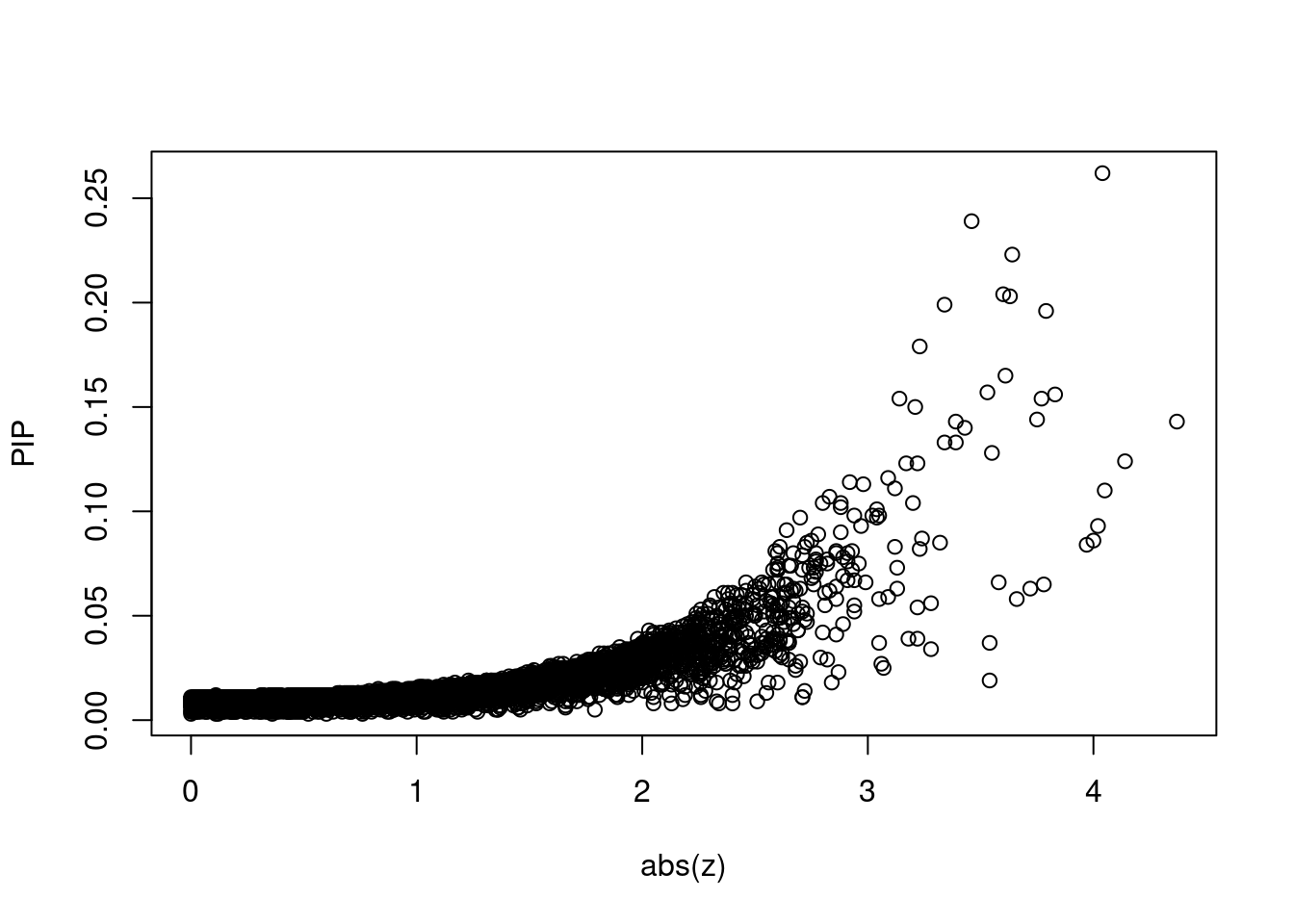
| Version | Author | Date |
|---|---|---|
| dfd2b5f | wesleycrouse | 2021-09-07 |
#proportion of significant z scores
mean(abs(ctwas_gene_res$z) > sig_thresh)
[1] 0#genes with most significant z scores
head(ctwas_gene_res[order(-abs(ctwas_gene_res$z)),report_cols],20) genename region_tag susie_pip mu2 PVE z
5042 SHROOM3 4_52 0.143 28.05 3.7e-05 4.37
9245 SETD2 3_33 0.124 25.87 3.0e-05 -4.14
7578 FRS2 12_43 0.110 24.32 2.5e-05 -4.05
7656 CATSPER2 15_16 0.262 30.13 7.3e-05 4.04
3715 SLC2A4RG 20_38 0.093 22.92 2.0e-05 4.02
10601 AGER 6_26 0.086 26.76 2.1e-05 -4.00
10186 ZGPAT 20_38 0.084 22.15 1.7e-05 3.97
10468 SFT2D1 6_108 0.156 25.07 3.6e-05 3.83
11448 INMT 7_24 0.196 30.66 5.5e-05 3.79
9992 FAM47E 4_52 0.065 22.09 1.3e-05 3.78
4888 CTDSPL2 15_17 0.154 25.09 3.6e-05 -3.77
2643 CCNC 6_67 0.144 27.28 3.6e-05 3.75
8970 PRSS42 3_33 0.063 20.84 1.2e-05 -3.72
1647 ARFRP1 20_38 0.058 19.46 1.0e-05 3.66
7269 TMEM184C 4_96 0.223 28.40 5.8e-05 -3.64
6602 HIST1H2BD 6_20 0.203 26.57 5.0e-05 3.63
12272 CTC-332L22.1 5_65 0.165 26.03 3.9e-05 -3.61
4061 NSUN5 7_47 0.204 27.81 5.2e-05 3.60
10629 CSNK2B 6_26 0.066 24.79 1.5e-05 3.58
593 MCM10 10_11 0.128 23.88 2.8e-05 -3.55Locus plots for genes and SNPs
ctwas_gene_res_sortz <- ctwas_gene_res[order(-abs(ctwas_gene_res$z)),]

n_plots <- 5
for (region_tag_plot in head(unique(ctwas_gene_res_sortz$region_tag), n_plots)){
  ctwas_res_region <-  ctwas_res[ctwas_res$region_tag==region_tag_plot,]
  start <- min(ctwas_res_region$pos)
  end <- max(ctwas_res_region$pos)

  ctwas_res_region <- ctwas_res_region[order(ctwas_res_region$pos),]
  ctwas_res_region_gene <- ctwas_res_region[ctwas_res_region$type=="gene",]
  ctwas_res_region_snp <- ctwas_res_region[ctwas_res_region$type=="SNP",]

  #region name
  print(paste0("Region: ", region_tag_plot))

  #table of genes in region
  print(ctwas_res_region_gene[,report_cols])

  par(mfrow=c(4,1))

  #gene z scores
  plot(ctwas_res_region_gene$pos, abs(ctwas_res_region_gene$z), xlab="Position", ylab="abs(gene_z)", xlim=c(start,end),
   ylim=c(0,max(sig_thresh, abs(ctwas_res_region_gene$z))),
   main=paste0("Region: ", region_tag_plot))
  abline(h=sig_thresh,col="red",lty=2)

  #significance threshold for SNPs
  alpha_snp <- 5*10^(-8)
  sig_thresh_snp <- qnorm(1-alpha_snp/2, lower=T)

  #snp z scores
  plot(ctwas_res_region_snp$pos, abs(ctwas_res_region_snp$z), xlab="Position", ylab="abs(snp_z)",xlim=c(start,end),
   ylim=c(0,max(sig_thresh_snp, max(abs(ctwas_res_region_snp$z)))))
  abline(h=sig_thresh_snp,col="purple",lty=2)

  #gene pips
  plot(ctwas_res_region_gene$pos, ctwas_res_region_gene$susie_pip, xlab="Position", ylab="Gene PIP", xlim=c(start,end), ylim=c(0,1))
  abline(h=0.8,col="blue",lty=2)

  #snp pips
  plot(ctwas_res_region_snp$pos, ctwas_res_region_snp$susie_pip, xlab="Position", ylab="SNP PIP", xlim=c(start,end), ylim=c(0,1))
  abline(h=0.8,col="blue",lty=2)
}
[1] "Region: 4_52"
genename region_tag susie_pip mu2 PVE z
5038 SCARB2 4_52 0.006 4.16 2.1e-07 0.62
9992 FAM47E 4_52 0.065 22.09 1.3e-05 3.78
7163 CCDC158 4_52 0.009 8.05 7.0e-07 2.33
5042 SHROOM3 4_52 0.143 28.05 3.7e-05 4.37
5036 SEPT11 4_52 0.006 4.65 2.5e-07 0.60
9710 SOWAHB 4_52 0.005 4.11 2.1e-07 0.41
3202 CCNI 4_52 0.005 4.03 2.0e-07 0.41
5039 CCNG2 4_52 0.005 3.93 1.9e-07 -0.38
5040 CNOT6L 4_52 0.005 3.78 1.8e-07 -0.30
8048 MRPL1 4_52 0.017 12.48 2.0e-06 2.08
5037 FRAS1 4_52 0.005 3.62 1.7e-07 -0.21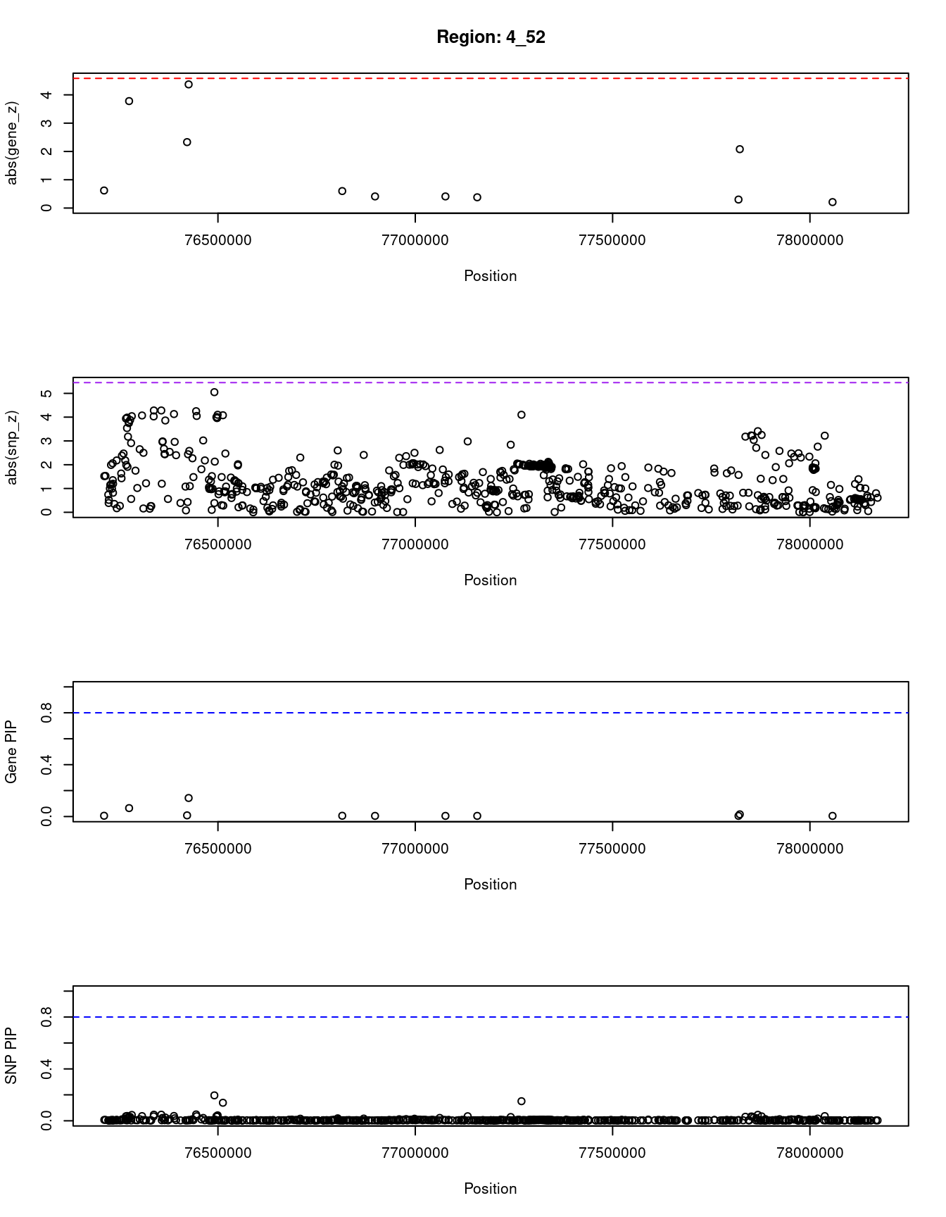
| Version | Author | Date |
|---|---|---|
| dfd2b5f | wesleycrouse | 2021-09-07 |
[1] "Region: 3_33"
      genename region_tag susie_pip   mu2     PVE     z
8968    ALS2CL       3_33     0.019 12.11 2.1e-06 -2.39
12003   PRSS46       3_33     0.008  5.66 4.1e-07  1.28
9872    PRSS45       3_33     0.024 13.70 3.0e-06  2.68
8970    PRSS42       3_33     0.063 20.84 1.2e-05 -3.72
6801     PTH1R       3_33     0.006  3.64 2.0e-07  0.09
6802      MYL3       3_33     0.009  6.92 6.0e-07 -1.36
6800    CCDC12       3_33     0.018 11.56 1.9e-06 -2.56
9245     SETD2       3_33     0.124 25.87 3.0e-05 -4.14
2834    KLHL18       3_33     0.022 12.94 2.6e-06 -2.42
2835      SCAP       3_33     0.037 16.92 5.8e-06  3.05
2833     CSPG5       3_33     0.066 21.15 1.3e-05  2.99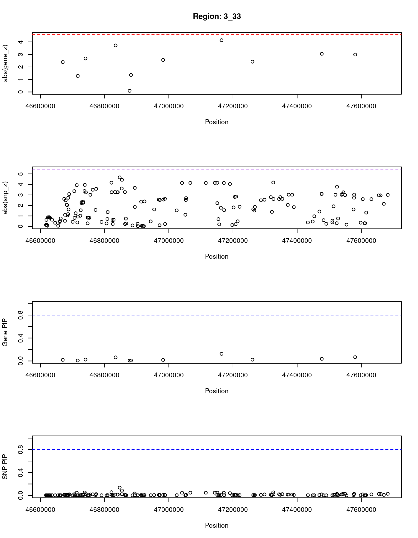
| Version | Author | Date |
|---|---|---|
| dfd2b5f | wesleycrouse | 2021-09-07 |
[1] "Region: 12_43"
     genename region_tag susie_pip   mu2     PVE     z
7578     FRS2      12_43     0.110 24.32 2.5e-05 -4.05
7579     CCT2      12_43     0.007  4.37 2.9e-07 -0.55
3849   RAB3IP      12_43     0.017 10.51 1.6e-06 -1.94
7587    MYRFL      12_43     0.026 13.79 3.3e-06 -2.46
2566    CNOT2      12_43     0.012  7.98 8.7e-07 -1.94
4617   KCNMB4      12_43     0.007  3.78 2.3e-07  0.27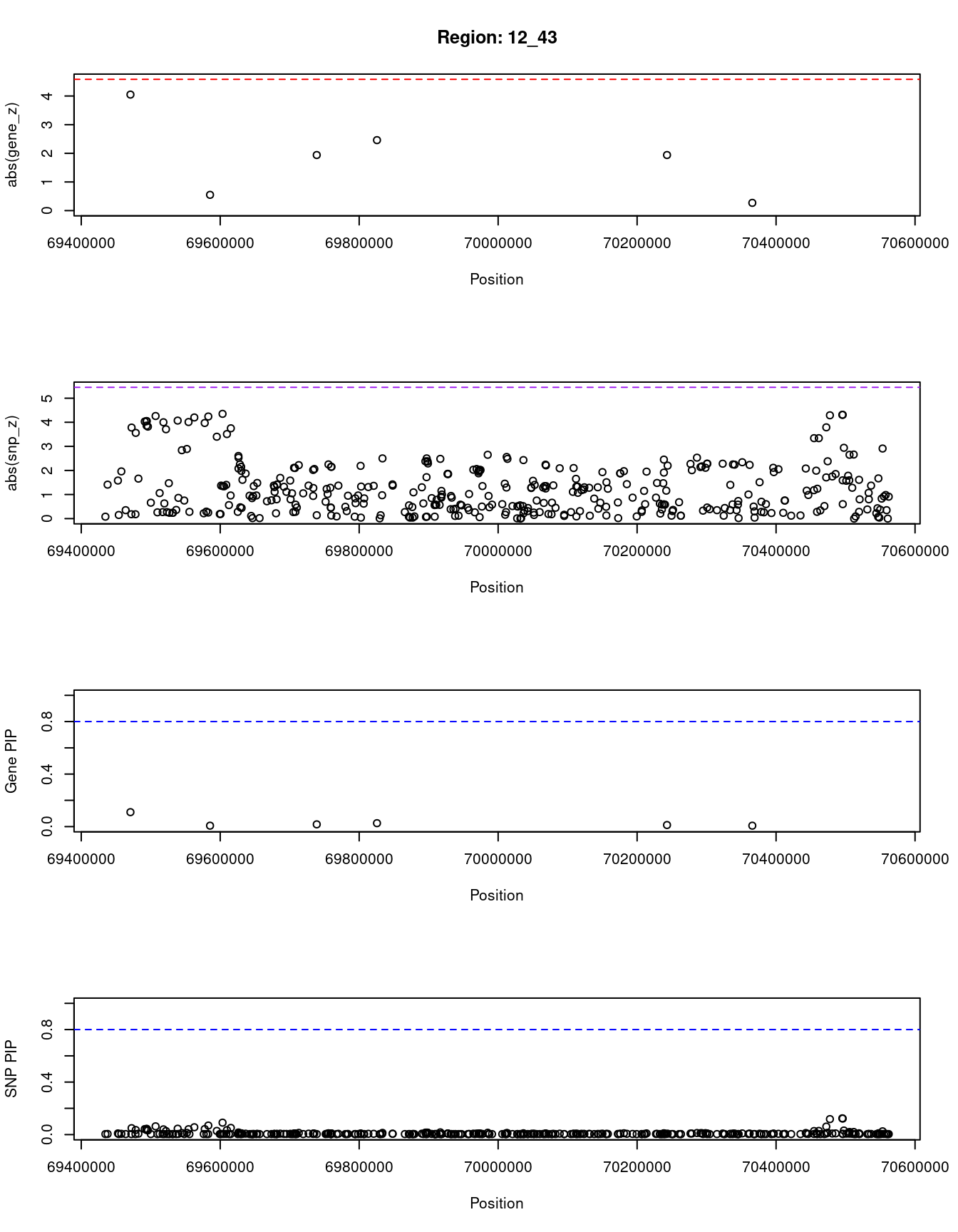
| Version | Author | Date |
|---|---|---|
| dfd2b5f | wesleycrouse | 2021-09-07 |
[1] "Region: 15_16"
     genename region_tag susie_pip   mu2     PVE     z
1853   ZNF106      15_16     0.019 10.33 1.8e-06 -1.87
9202   LRRC57      15_16     0.022 11.50 2.3e-06  1.94
6691   STARD9      15_16     0.010  5.89 5.5e-07 -1.14
5189    CDAN1      15_16     0.157 26.07 3.8e-05  3.53
3962    TTBK2      15_16     0.009  5.02 4.2e-07 -0.97
4903   TMEM62      15_16     0.010  5.97 5.7e-07 -1.16
7984     ADAL      15_16     0.009  4.60 3.6e-07  0.23
7985    LCMT2      15_16     0.017  9.63 1.5e-06 -2.17
4898  TUBGCP4      15_16     0.007  3.67 2.5e-07  0.58
5180  ZSCAN29      15_16     0.008  3.97 2.9e-07 -0.56
7702    MAP1A      15_16     0.010  5.46 4.8e-07  1.36
7656 CATSPER2      15_16     0.262 30.13 7.3e-05  4.04
7709    PDIA3      15_16     0.008  4.11 3.0e-07  0.69
5178    MFAP1      15_16     0.008  4.13 3.0e-07  0.90
1286    WDR76      15_16     0.008  3.84 2.7e-07  0.71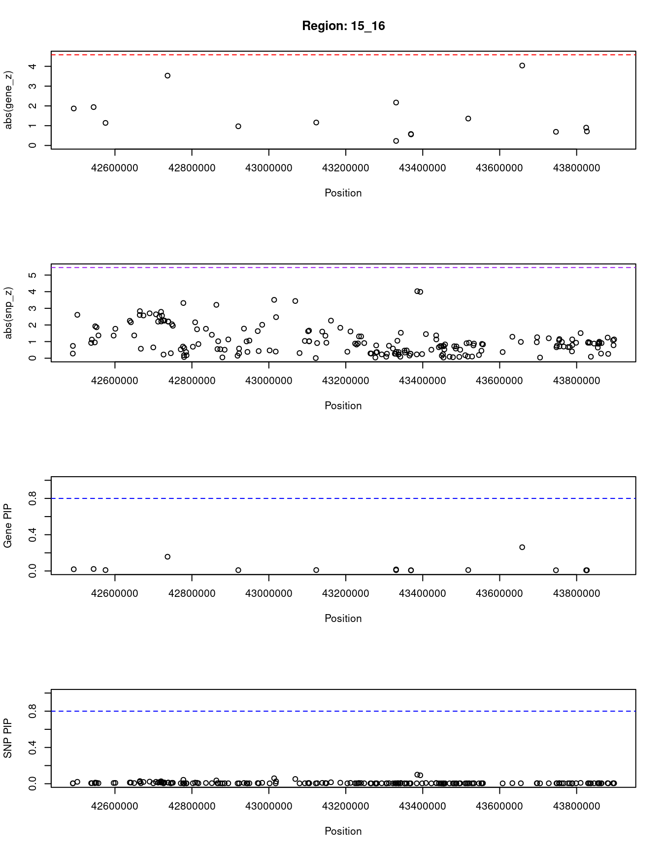
| Version | Author | Date |
|---|---|---|
| dfd2b5f | wesleycrouse | 2021-09-07 |
[1] "Region: 20_38"
       genename region_tag susie_pip   mu2     PVE     z
4090      HELZ2      20_38     0.007  4.06 2.6e-07 -0.41
1641      GMEB2      20_38     0.014  8.88 1.1e-06 -2.28
10242     STMN3      20_38     0.007  3.61 2.2e-07  0.20
11853     RTEL1      20_38     0.008  4.85 3.5e-07  1.46
1647     ARFRP1      20_38     0.058 19.46 1.0e-05  3.66
10186     ZGPAT      20_38     0.084 22.15 1.7e-05  3.97
10551     LIME1      20_38     0.007  3.84 2.4e-07  0.71
3715   SLC2A4RG      20_38     0.093 22.92 2.0e-05  4.02
1624    TPD52L2      20_38     0.031 14.75 4.2e-06 -2.16
1625     DNAJC5      20_38     0.039 16.49 5.9e-06 -2.61
10130   ZNF512B      20_38     0.018 11.01 1.9e-06 -1.77
4091     SAMD10      20_38     0.054 18.83 9.3e-06  2.71
1627      PRPF6      20_38     0.016 10.04 1.5e-06 -1.63
10078 LINC00176      20_38     0.007  3.64 2.2e-07  0.07
8346      TCEA2      20_38     0.008  5.05 3.8e-07 -1.01
8345      RGS19      20_38     0.007  4.05 2.6e-07  0.39
10024      MYT1      20_38     0.009  5.98 5.1e-07  1.03
10550    PCMTD2      20_38     0.021 11.82 2.2e-06  1.98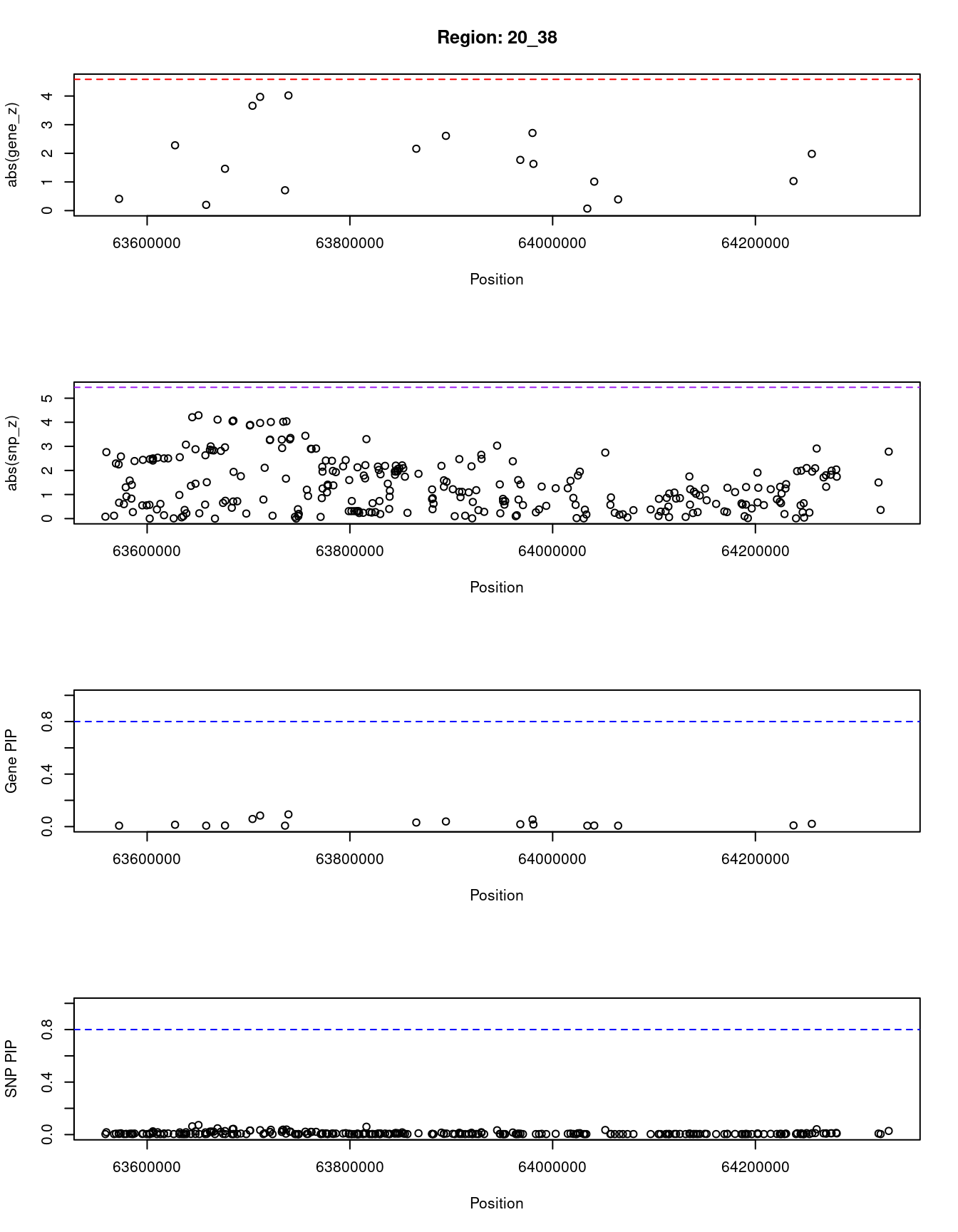
| Version | Author | Date |
|---|---|---|
| dfd2b5f | wesleycrouse | 2021-09-07 |
SNPs with highest PIPs
#snps with PIP>0.8 or 20 highest PIPs
head(ctwas_snp_res[order(-ctwas_snp_res$susie_pip),report_cols_snps],
max(sum(ctwas_snp_res$susie_pip>0.8), 20))
id region_tag susie_pip mu2 PVE z
265377 rs4109437 4_122 1.000 54.73 5.0e-04 9.52
524158 rs17343073 10_14 0.928 52.11 4.4e-04 9.45
72021 rs17432480 2_9 0.400 31.75 1.2e-04 -4.80
250242 rs6857487 4_96 0.368 31.65 1.1e-04 4.86
13754 rs7543243 1_29 0.352 32.02 1.0e-04 5.12
235650 rs1508422 4_67 0.292 30.67 8.2e-05 -4.63
319239 rs116004855 5_104 0.287 29.46 7.8e-05 4.29
160246 rs774067422 3_42 0.282 28.63 7.4e-05 4.46
838797 rs8117150 20_27 0.259 28.20 6.7e-05 4.12
100467 rs1898846 2_66 0.249 30.40 7.0e-05 -4.76
524165 rs113795872 10_14 0.244 50.33 1.1e-04 9.02
526099 rs551737161 10_16 0.239 31.16 6.8e-05 -3.38
231831 rs60955950 4_60 0.237 28.48 6.2e-05 -4.35
24492 rs59104377 1_51 0.234 27.62 5.9e-05 -4.09
467073 rs138854257 8_70 0.232 27.86 5.9e-05 4.14
460516 rs16907708 8_57 0.231 29.21 6.2e-05 -4.22
549774 rs11189853 10_63 0.224 27.57 5.7e-05 3.99
739370 rs35419776 16_17 0.224 27.72 5.7e-05 -4.05
848984 rs191739247 21_7 0.221 27.02 5.5e-05 3.93
52803 rs600396 1_105 0.220 27.45 5.6e-05 4.06SNPs with largest effect sizes
#plot PIP vs effect size
plot(ctwas_snp_res$susie_pip, ctwas_snp_res$mu2, xlab="PIP", ylab="mu^2", main="SNP PIPs vs Effect Size")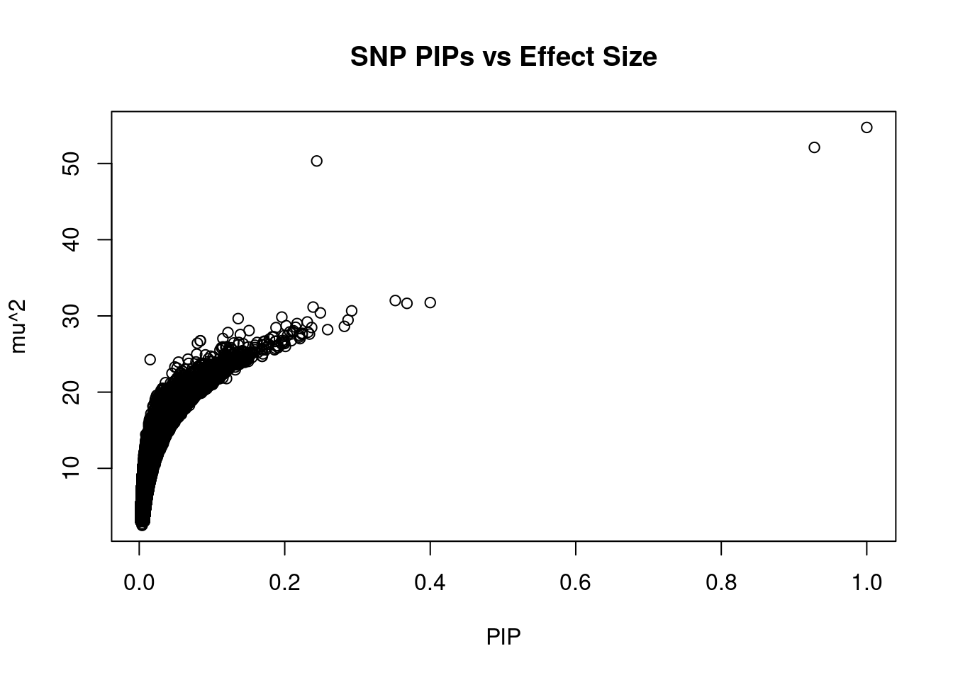
| Version | Author | Date |
|---|---|---|
| dfd2b5f | wesleycrouse | 2021-09-07 |
#SNPs with 50 largest effect sizes
head(ctwas_snp_res[order(-ctwas_snp_res$mu2),report_cols_snps],50)
id region_tag susie_pip mu2 PVE z
265377 rs4109437 4_122 1.000 54.73 5.0e-04 9.52
524158 rs17343073 10_14 0.928 52.11 4.4e-04 9.45
524165 rs113795872 10_14 0.244 50.33 1.1e-04 9.02
13754 rs7543243 1_29 0.352 32.02 1.0e-04 5.12
72021 rs17432480 2_9 0.400 31.75 1.2e-04 -4.80
250242 rs6857487 4_96 0.368 31.65 1.1e-04 4.86
526099 rs551737161 10_16 0.239 31.16 6.8e-05 -3.38
235650 rs1508422 4_67 0.292 30.67 8.2e-05 -4.63
100467 rs1898846 2_66 0.249 30.40 7.0e-05 -4.76
228055 rs13146163 4_52 0.196 29.85 5.4e-05 -5.05
334929 rs16869385 6_26 0.136 29.65 3.7e-05 4.58
319239 rs116004855 5_104 0.287 29.46 7.8e-05 4.29
460516 rs16907708 8_57 0.231 29.21 6.2e-05 -4.22
744211 rs12927956 16_27 0.217 29.00 5.8e-05 4.12
570432 rs118142338 11_17 0.202 28.72 5.3e-05 -4.03
160246 rs774067422 3_42 0.282 28.63 7.4e-05 4.46
13745 rs2065944 1_29 0.215 28.51 5.6e-05 4.53
231831 rs60955950 4_60 0.237 28.48 6.2e-05 -4.35
100473 rs4848374 2_66 0.188 28.47 4.9e-05 -4.62
838797 rs8117150 20_27 0.259 28.20 6.7e-05 4.12
228335 rs2194125 4_52 0.151 28.08 3.9e-05 -4.10
279316 rs13179493 5_26 0.212 28.06 5.5e-05 -4.60
788005 rs138729533 18_12 0.211 27.90 5.4e-05 4.07
828978 rs1987579 20_5 0.207 27.90 5.3e-05 4.11
467073 rs138854257 8_70 0.232 27.86 5.9e-05 4.14
796375 rs1443568 18_28 0.122 27.82 3.1e-05 4.07
739370 rs35419776 16_17 0.224 27.72 5.7e-05 -4.05
853043 rs73352324 21_15 0.210 27.64 5.4e-05 -4.33
24492 rs59104377 1_51 0.234 27.62 5.9e-05 -4.09
549774 rs11189853 10_63 0.224 27.57 5.7e-05 3.99
228067 rs147760951 4_52 0.139 27.56 3.5e-05 -4.08
52803 rs600396 1_105 0.220 27.45 5.6e-05 4.06
534353 rs116858637 10_33 0.204 27.45 5.2e-05 -3.95
662569 rs79125844 13_32 0.199 27.40 5.0e-05 4.21
499269 rs1175334 9_39 0.185 27.27 4.6e-05 -4.27
713324 rs8033332 15_15 0.183 27.26 4.6e-05 -4.65
412256 rs6958957 7_56 0.220 27.23 5.5e-05 4.00
451164 rs139902438 8_40 0.115 27.03 2.8e-05 4.10
848984 rs191739247 21_7 0.221 27.02 5.5e-05 3.93
519225 rs10795199 10_6 0.179 26.96 4.5e-05 4.02
819757 rs146928263 19_27 0.197 26.78 4.9e-05 -3.93
290066 rs7716273 5_46 0.209 26.75 5.1e-05 -4.16
334505 rs13215664 6_25 0.084 26.74 2.1e-05 5.09
334506 rs4991645 6_25 0.084 26.73 2.1e-05 5.09
522764 rs7090451 10_11 0.188 26.70 4.6e-05 -4.38
133887 rs79567528 2_133 0.172 26.69 4.2e-05 -4.29
792180 rs12458728 18_21 0.199 26.67 4.9e-05 -3.94
522762 rs6602637 10_11 0.187 26.65 4.6e-05 -4.38
786058 rs1160103 18_8 0.171 26.60 4.2e-05 4.10
56561 rs552055532 1_111 0.199 26.52 4.9e-05 -3.85SNPs with highest PVE
#SNPs with 50 highest pve
head(ctwas_snp_res[order(-ctwas_snp_res$PVE),report_cols_snps],50)
id region_tag susie_pip mu2 PVE z
265377 rs4109437 4_122 1.000 54.73 5.0e-04 9.52
524158 rs17343073 10_14 0.928 52.11 4.4e-04 9.45
72021 rs17432480 2_9 0.400 31.75 1.2e-04 -4.80
250242 rs6857487 4_96 0.368 31.65 1.1e-04 4.86
524165 rs113795872 10_14 0.244 50.33 1.1e-04 9.02
13754 rs7543243 1_29 0.352 32.02 1.0e-04 5.12
235650 rs1508422 4_67 0.292 30.67 8.2e-05 -4.63
319239 rs116004855 5_104 0.287 29.46 7.8e-05 4.29
160246 rs774067422 3_42 0.282 28.63 7.4e-05 4.46
100467 rs1898846 2_66 0.249 30.40 7.0e-05 -4.76
526099 rs551737161 10_16 0.239 31.16 6.8e-05 -3.38
838797 rs8117150 20_27 0.259 28.20 6.7e-05 4.12
231831 rs60955950 4_60 0.237 28.48 6.2e-05 -4.35
460516 rs16907708 8_57 0.231 29.21 6.2e-05 -4.22
24492 rs59104377 1_51 0.234 27.62 5.9e-05 -4.09
467073 rs138854257 8_70 0.232 27.86 5.9e-05 4.14
744211 rs12927956 16_27 0.217 29.00 5.8e-05 4.12
549774 rs11189853 10_63 0.224 27.57 5.7e-05 3.99
739370 rs35419776 16_17 0.224 27.72 5.7e-05 -4.05
13745 rs2065944 1_29 0.215 28.51 5.6e-05 4.53
52803 rs600396 1_105 0.220 27.45 5.6e-05 4.06
279316 rs13179493 5_26 0.212 28.06 5.5e-05 -4.60
412256 rs6958957 7_56 0.220 27.23 5.5e-05 4.00
848984 rs191739247 21_7 0.221 27.02 5.5e-05 3.93
228055 rs13146163 4_52 0.196 29.85 5.4e-05 -5.05
788005 rs138729533 18_12 0.211 27.90 5.4e-05 4.07
853043 rs73352324 21_15 0.210 27.64 5.4e-05 -4.33
570432 rs118142338 11_17 0.202 28.72 5.3e-05 -4.03
828978 rs1987579 20_5 0.207 27.90 5.3e-05 4.11
534353 rs116858637 10_33 0.204 27.45 5.2e-05 -3.95
290066 rs7716273 5_46 0.209 26.75 5.1e-05 -4.16
662569 rs79125844 13_32 0.199 27.40 5.0e-05 4.21
56561 rs552055532 1_111 0.199 26.52 4.9e-05 -3.85
100473 rs4848374 2_66 0.188 28.47 4.9e-05 -4.62
792180 rs12458728 18_21 0.199 26.67 4.9e-05 -3.94
819757 rs146928263 19_27 0.197 26.78 4.9e-05 -3.93
313386 rs186927917 5_91 0.200 26.38 4.8e-05 3.82
530237 rs79262861 10_25 0.201 26.00 4.8e-05 -3.89
811724 rs199991194 19_12 0.196 26.29 4.7e-05 3.85
179917 rs112861149 3_80 0.191 26.06 4.6e-05 3.91
499269 rs1175334 9_39 0.185 27.27 4.6e-05 -4.27
522762 rs6602637 10_11 0.187 26.65 4.6e-05 -4.38
522764 rs7090451 10_11 0.188 26.70 4.6e-05 -4.38
713324 rs8033332 15_15 0.183 27.26 4.6e-05 -4.65
267915 rs77497829 5_5 0.191 25.85 4.5e-05 3.79
519225 rs10795199 10_6 0.179 26.96 4.5e-05 4.02
551652 rs10509810 10_67 0.188 26.07 4.5e-05 -4.02
619672 rs117751804 12_29 0.187 25.75 4.4e-05 -3.92
637241 rs11112070 12_63 0.186 25.56 4.4e-05 -3.81
625193 rs138600567 12_40 0.178 26.27 4.3e-05 -3.80SNPs with largest z scores
#SNPs with 50 largest z scores
head(ctwas_snp_res[order(-abs(ctwas_snp_res$z)),report_cols_snps],50)
id region_tag susie_pip mu2 PVE z
265377 rs4109437 4_122 1.000 54.73 5.0e-04 9.52
524158 rs17343073 10_14 0.928 52.11 4.4e-04 9.45
524165 rs113795872 10_14 0.244 50.33 1.1e-04 9.02
524169 rs3858184 10_14 0.015 24.27 3.4e-06 6.34
13754 rs7543243 1_29 0.352 32.02 1.0e-04 5.12
334505 rs13215664 6_25 0.084 26.74 2.1e-05 5.09
334506 rs4991645 6_25 0.084 26.73 2.1e-05 5.09
228055 rs13146163 4_52 0.196 29.85 5.4e-05 -5.05
334512 rs2395492 6_25 0.080 26.42 1.9e-05 4.99
565641 rs61889814 11_8 0.130 26.45 3.2e-05 4.99
565639 rs59090117 11_8 0.120 25.95 2.9e-05 4.96
565637 rs55879783 11_8 0.119 25.90 2.8e-05 4.95
250242 rs6857487 4_96 0.368 31.65 1.1e-04 4.86
72021 rs17432480 2_9 0.400 31.75 1.2e-04 -4.80
100467 rs1898846 2_66 0.249 30.40 7.0e-05 -4.76
155840 rs73065135 3_33 0.137 26.52 3.3e-05 4.67
713324 rs8033332 15_15 0.183 27.26 4.6e-05 -4.65
334338 rs34548997 6_25 0.054 23.94 1.2e-05 4.64
235650 rs1508422 4_67 0.292 30.67 8.2e-05 -4.63
100473 rs4848374 2_66 0.188 28.47 4.9e-05 -4.62
279316 rs13179493 5_26 0.212 28.06 5.5e-05 -4.60
334373 rs6929132 6_25 0.049 23.30 1.1e-05 4.59
334929 rs16869385 6_26 0.136 29.65 3.7e-05 4.58
13745 rs2065944 1_29 0.215 28.51 5.6e-05 4.53
13757 rs6681140 1_29 0.127 24.97 2.9e-05 4.53
334562 rs542630771 6_25 0.026 19.16 4.5e-06 4.47
542391 rs7909516 10_49 0.169 26.23 4.1e-05 4.47
740076 rs35830321 16_19 0.154 25.19 3.6e-05 -4.47
160246 rs774067422 3_42 0.282 28.63 7.4e-05 4.46
334559 rs7752021 6_25 0.025 19.08 4.4e-06 4.46
334561 rs75098758 6_25 0.025 19.07 4.4e-06 4.46
334558 rs7771971 6_25 0.025 19.00 4.4e-06 4.45
334565 rs67484745 6_25 0.025 18.98 4.4e-06 4.45
334566 rs150737002 6_25 0.025 19.02 4.4e-06 4.45
155842 rs6768845 3_33 0.086 23.50 1.9e-05 4.44
542389 rs4531409 10_49 0.159 25.84 3.8e-05 4.44
334546 rs73398308 6_25 0.024 18.77 4.2e-06 4.43
334537 rs28623422 6_25 0.023 18.61 4.0e-06 4.42
334544 rs13437094 6_25 0.023 18.61 4.0e-06 4.42
713327 rs7183231 15_15 0.118 24.34 2.6e-05 4.42
713351 rs28810086 15_15 0.131 25.00 3.0e-05 4.42
193145 rs9865575 3_105 0.137 24.93 3.1e-05 4.41
334567 rs66862067 6_25 0.023 18.54 4.0e-06 4.41
379190 rs34430737 6_108 0.159 25.28 3.7e-05 4.40
471489 rs55781186 8_79 0.169 25.53 4.0e-05 4.39
522762 rs6602637 10_11 0.187 26.65 4.6e-05 -4.38
522764 rs7090451 10_11 0.188 26.70 4.6e-05 -4.38
193147 rs73171228 3_105 0.128 24.47 2.9e-05 4.37
542390 rs765918 10_49 0.140 24.96 3.2e-05 4.37
193148 rs6808176 3_105 0.127 24.40 2.8e-05 4.36Gene set enrichment for genes with PIP>0.8
#GO enrichment analysis
library(enrichR)
Welcome to enrichR
Checking connection ... Enrichr ... Connection is Live!
FlyEnrichr ... Connection is available!
WormEnrichr ... Connection is available!
YeastEnrichr ... Connection is available!
FishEnrichr ... Connection is available!dbs <- c("GO_Biological_Process_2021", "GO_Cellular_Component_2021", "GO_Molecular_Function_2021")
genes <- ctwas_gene_res$genename[ctwas_gene_res$susie_pip>0.8]
#number of genes for gene set enrichment
length(genes)[1] 0if (length(genes)>0){
GO_enrichment <- enrichr(genes, dbs)
for (db in dbs){
print(db)
df <- GO_enrichment[[db]]
df <- df[df$Adjusted.P.value<0.05,c("Term", "Overlap", "Adjusted.P.value", "Genes")]
print(df)
}
#DisGeNET enrichment
# devtools::install_bitbucket("ibi_group/disgenet2r")
library(disgenet2r)
disgenet_api_key <- get_disgenet_api_key(
email = "wesleycrouse@gmail.com",
password = "uchicago1" )
Sys.setenv(DISGENET_API_KEY= disgenet_api_key)
res_enrich <-disease_enrichment(entities=genes, vocabulary = "HGNC",
database = "CURATED" )
df <- res_enrich@qresult[1:10, c("Description", "FDR", "Ratio", "BgRatio")]
print(df)
#WebGestalt enrichment
library(WebGestaltR)
background <- ctwas_gene_res$genename
#listGeneSet()
databases <- c("pathway_KEGG", "disease_GLAD4U", "disease_OMIM")
enrichResult <- WebGestaltR(enrichMethod="ORA", organism="hsapiens",
interestGene=genes, referenceGene=background,
enrichDatabase=databases, interestGeneType="genesymbol",
referenceGeneType="genesymbol", isOutput=F)
print(enrichResult[,c("description", "size", "overlap", "FDR", "database", "userId")])
}
sessionInfo()R version 3.6.1 (2019-07-05)
Platform: x86_64-pc-linux-gnu (64-bit)
Running under: Scientific Linux 7.4 (Nitrogen)
Matrix products: default
BLAS/LAPACK: /software/openblas-0.2.19-el7-x86_64/lib/libopenblas_haswellp-r0.2.19.so
locale:
[1] LC_CTYPE=en_US.UTF-8 LC_NUMERIC=C
[3] LC_TIME=en_US.UTF-8 LC_COLLATE=en_US.UTF-8
[5] LC_MONETARY=en_US.UTF-8 LC_MESSAGES=en_US.UTF-8
[7] LC_PAPER=en_US.UTF-8 LC_NAME=C
[9] LC_ADDRESS=C LC_TELEPHONE=C
[11] LC_MEASUREMENT=en_US.UTF-8 LC_IDENTIFICATION=C
attached base packages:
[1] stats graphics grDevices utils datasets methods base
other attached packages:
[1] enrichR_3.0 cowplot_1.0.0 ggplot2_3.3.3
loaded via a namespace (and not attached):
[1] Biobase_2.44.0 httr_1.4.1
[3] bit64_4.0.5 assertthat_0.2.1
[5] stats4_3.6.1 blob_1.2.1
[7] BSgenome_1.52.0 GenomeInfoDbData_1.2.1
[9] Rsamtools_2.0.0 yaml_2.2.0
[11] progress_1.2.2 pillar_1.6.1
[13] RSQLite_2.2.7 lattice_0.20-38
[15] glue_1.4.2 digest_0.6.20
[17] GenomicRanges_1.36.0 promises_1.0.1
[19] XVector_0.24.0 colorspace_1.4-1
[21] htmltools_0.3.6 httpuv_1.5.1
[23] Matrix_1.2-18 XML_3.98-1.20
[25] pkgconfig_2.0.3 biomaRt_2.40.1
[27] zlibbioc_1.30.0 purrr_0.3.4
[29] scales_1.1.0 whisker_0.3-2
[31] later_0.8.0 BiocParallel_1.18.0
[33] git2r_0.26.1 tibble_3.1.2
[35] farver_2.1.0 generics_0.0.2
[37] IRanges_2.18.1 ellipsis_0.3.2
[39] withr_2.4.1 cachem_1.0.5
[41] SummarizedExperiment_1.14.1 GenomicFeatures_1.36.3
[43] BiocGenerics_0.30.0 magrittr_2.0.1
[45] crayon_1.4.1 memoise_2.0.0
[47] evaluate_0.14 fs_1.3.1
[49] fansi_0.5.0 tools_3.6.1
[51] data.table_1.14.0 prettyunits_1.0.2
[53] hms_1.1.0 lifecycle_1.0.0
[55] matrixStats_0.57.0 stringr_1.4.0
[57] S4Vectors_0.22.1 munsell_0.5.0
[59] DelayedArray_0.10.0 AnnotationDbi_1.46.0
[61] Biostrings_2.52.0 compiler_3.6.1
[63] GenomeInfoDb_1.20.0 rlang_0.4.11
[65] grid_3.6.1 RCurl_1.98-1.1
[67] rjson_0.2.20 VariantAnnotation_1.30.1
[69] labeling_0.3 bitops_1.0-6
[71] rmarkdown_1.13 gtable_0.3.0
[73] curl_3.3 DBI_1.1.1
[75] R6_2.5.0 GenomicAlignments_1.20.1
[77] dplyr_1.0.7 knitr_1.23
[79] rtracklayer_1.44.0 utf8_1.2.1
[81] fastmap_1.1.0 bit_4.0.4
[83] workflowr_1.6.2 rprojroot_2.0.2
[85] stringi_1.4.3 parallel_3.6.1
[87] Rcpp_1.0.6 vctrs_0.3.8
[89] tidyselect_1.1.0 xfun_0.8