Diagnoses - main ICD10: K50 Crohn’s disease [regional enteritis] - all weights
wesleycrouse
2022-02-28
Last updated: 2022-03-22
Checks: 7 0
Knit directory: ctwas_applied/
This reproducible R Markdown analysis was created with workflowr (version 1.6.2). The Checks tab describes the reproducibility checks that were applied when the results were created. The Past versions tab lists the development history.
Great! Since the R Markdown file has been committed to the Git repository, you know the exact version of the code that produced these results.
Great job! The global environment was empty. Objects defined in the global environment can affect the analysis in your R Markdown file in unknown ways. For reproduciblity it’s best to always run the code in an empty environment.
The command set.seed(20210726) was run prior to running the code in the R Markdown file. Setting a seed ensures that any results that rely on randomness, e.g. subsampling or permutations, are reproducible.
Great job! Recording the operating system, R version, and package versions is critical for reproducibility.
Nice! There were no cached chunks for this analysis, so you can be confident that you successfully produced the results during this run.
Great job! Using relative paths to the files within your workflowr project makes it easier to run your code on other machines.
Great! You are using Git for version control. Tracking code development and connecting the code version to the results is critical for reproducibility.
The results in this page were generated with repository version 073f2a3. See the Past versions tab to see a history of the changes made to the R Markdown and HTML files.
Note that you need to be careful to ensure that all relevant files for the analysis have been committed to Git prior to generating the results (you can use wflow_publish or wflow_git_commit). workflowr only checks the R Markdown file, but you know if there are other scripts or data files that it depends on. Below is the status of the Git repository when the results were generated:
working directory clean
Note that any generated files, e.g. HTML, png, CSS, etc., are not included in this status report because it is ok for generated content to have uncommitted changes.
These are the previous versions of the repository in which changes were made to the R Markdown (analysis/ukb-a-552_allweights.Rmd) and HTML (docs/ukb-a-552_allweights.html) files. If you’ve configured a remote Git repository (see ?wflow_git_remote), click on the hyperlinks in the table below to view the files as they were in that past version.
| File | Version | Author | Date | Message |
|---|---|---|---|---|
| Rmd | 073f2a3 | wesleycrouse | 2022-03-22 | enrichment analysis for all weights |
| Rmd | ba908fe | wesleycrouse | 2022-03-21 | more traits for all weight analysis |
trait_id <- "ukb-a-552"
trait_name <- "Diagnoses - main ICD10: K50 Crohn's disease [regional enteritis]"

source("/project2/mstephens/wcrouse/UKB_analysis_allweights/ctwas_config.R")

trait_dir <- paste0("/project2/mstephens/wcrouse/UKB_analysis_allweights/", trait_id)

results_dirs <- list.dirs(trait_dir, recursive=F)
Load cTWAS results for all weights
# df <- list()
#
# for (i in 1:length(results_dirs)){
#   print(i)
#
#   results_dir <- results_dirs[i]
#   weight <- rev(unlist(strsplit(results_dir, "/")))[1]
#   analysis_id <- paste(trait_id, weight, sep="_")
#
#   #load ctwas results
#   ctwas_res <- data.table::fread(paste0(results_dir, "/", analysis_id, "_ctwas.susieIrss.txt"))
#
#   #make unique identifier for regions
#   ctwas_res$region_tag <- paste(ctwas_res$region_tag1, ctwas_res$region_tag2, sep="_")
#
#   #load z scores for SNPs and collect sample size
#   load(paste0(results_dir, "/", analysis_id, "_expr_z_snp.Rd"))
#
#   sample_size <- z_snp$ss
#   sample_size <- as.numeric(names(which.max(table(sample_size))))
#
#   #separate gene and SNP results
#   ctwas_gene_res <- ctwas_res[ctwas_res$type == "gene", ]
#   ctwas_gene_res <- data.frame(ctwas_gene_res)
#   ctwas_snp_res <- ctwas_res[ctwas_res$type == "SNP", ]
#   ctwas_snp_res <- data.frame(ctwas_snp_res)
#
#   #add gene information to results
#   sqlite <- RSQLite::dbDriver("SQLite")
#   db = RSQLite::dbConnect(sqlite, paste0("/project2/compbio/predictdb/mashr_models/mashr_", weight, ".db"))
#   query <- function(...) RSQLite::dbGetQuery(db, ...)
#   gene_info <- query("select gene, genename, gene_type from extra")
#   RSQLite::dbDisconnect(db)
#
#   ctwas_gene_res <- cbind(ctwas_gene_res, gene_info[sapply(ctwas_gene_res$id, match, gene_info$gene), c("genename", "gene_type")])
#
#   #add z scores to results
#   load(paste0(results_dir, "/", analysis_id, "_expr_z_gene.Rd"))
#   ctwas_gene_res$z <- z_gene[ctwas_gene_res$id,]$z
#
#   z_snp <- z_snp[z_snp$id %in% ctwas_snp_res$id,]
#   ctwas_snp_res$z <- z_snp$z[match(ctwas_snp_res$id, z_snp$id)]
#
#   #merge gene and snp results with added information
#   ctwas_snp_res$genename=NA
#   ctwas_snp_res$gene_type=NA
#
#   ctwas_res <- rbind(ctwas_gene_res,
#                    ctwas_snp_res[,colnames(ctwas_gene_res)])
#
#   #get number of SNPs from s1 results; adjust for thin argument
#   ctwas_res_s1 <- data.table::fread(paste0(results_dir, "/", analysis_id, "_ctwas.s1.susieIrss.txt"))
#   n_snps <- sum(ctwas_res_s1$type=="SNP")/thin
#   rm(ctwas_res_s1)
#
#   #load estimated parameters
#   load(paste0(results_dir, "/", analysis_id, "_ctwas.s2.susieIrssres.Rd"))
#
#   #estimated group prior
#   estimated_group_prior <- group_prior_rec[,ncol(group_prior_rec)]
#   names(estimated_group_prior) <- c("gene", "snp")
#   estimated_group_prior["snp"] <- estimated_group_prior["snp"]*thin #adjust parameter to account for thin argument
#
#   #estimated group prior variance
#   estimated_group_prior_var <- group_prior_var_rec[,ncol(group_prior_var_rec)]
#   names(estimated_group_prior_var) <- c("gene", "snp")
#
#   #report group size
#   group_size <- c(nrow(ctwas_gene_res), n_snps)
#
#   #estimated group PVE
#   estimated_group_pve <- estimated_group_prior_var*estimated_group_prior*group_size/sample_size
#   names(estimated_group_pve) <- c("gene", "snp")
#
#   #ctwas genes using PIP>0.8
#   ctwas_genes_index <- ctwas_gene_res$susie_pip>0.8
#   ctwas_genes <- ctwas_gene_res$genename[ctwas_genes_index]
#
#   #twas genes using bonferroni threshold
#   alpha <- 0.05
#   sig_thresh <- qnorm(1-(alpha/nrow(ctwas_gene_res)/2), lower=T)
#
#   twas_genes_index <- abs(ctwas_gene_res$z) > sig_thresh
#   twas_genes <- ctwas_gene_res$genename[twas_genes_index]
#
#   #gene PIPs and z scores
#   gene_pips <- ctwas_gene_res[,c("genename", "region_tag", "susie_pip", "z")]
#
#   #total PIPs by region
#
#   regions <- unique(ctwas_gene_res$region_tag)
#
#   region_pips <- data.frame(region=regions, stringsAsFactors=F)
#
#   region_pips$gene_pip <- sapply(regions, function(x){sum(ctwas_gene_res$susie_pip[ctwas_gene_res$region_tag==x])})
#   region_pips$snp_pip <- sapply(regions, function(x){sum(ctwas_snp_res$susie_pip[ctwas_snp_res$region_tag==x])})
#   region_pips$snp_maxz <- sapply(regions, function(x){max(abs(ctwas_snp_res$z[ctwas_snp_res$region_tag==x]))})
#
#   df[[weight]] <- list(prior=estimated_group_prior,
#                      prior_var=estimated_group_prior_var,
#                      pve=estimated_group_pve,
#                      ctwas=ctwas_genes,
#                      twas=twas_genes,
#                      gene_pips=gene_pips,
#                      region_pips=region_pips,
#                      sig_thresh=sig_thresh)
# }
#
# save(df, file=paste(trait_dir, "results_df.RData", sep="/"))
load(paste(trait_dir, "results_df.RData", sep="/"))

output <- data.frame(weight=names(df),
                     prior_g=unlist(lapply(df, function(x){x$prior["gene"]})),
                     prior_s=unlist(lapply(df, function(x){x$prior["snp"]})),
                     prior_var_g=unlist(lapply(df, function(x){x$prior_var["gene"]})),
                     prior_var_s=unlist(lapply(df, function(x){x$prior_var["snp"]})),
                     pve_g=unlist(lapply(df, function(x){x$pve["gene"]})),
                     pve_s=unlist(lapply(df, function(x){x$pve["snp"]})),
                     n_ctwas=unlist(lapply(df, function(x){length(x$ctwas)})),
                     n_twas=unlist(lapply(df, function(x){length(x$twas)})),
                     row.names=NULL,
                     stringsAsFactors=F)
Plot estimated prior parameters and PVE
#plot estimated group prior

output <- output[order(-output$prior_g),]

par(mar=c(10.1, 4.1, 4.1, 2.1))

plot(output$prior_g, type="l", ylim=c(0, max(output$prior_g, output$prior_s)*1.1),
     xlab="", ylab="Estimated Group Prior", xaxt = "n", col="blue")
lines(output$prior_s)

axis(1, at = 1:nrow(output),
     labels = output$weight,
     las=2,
     cex.axis=0.6)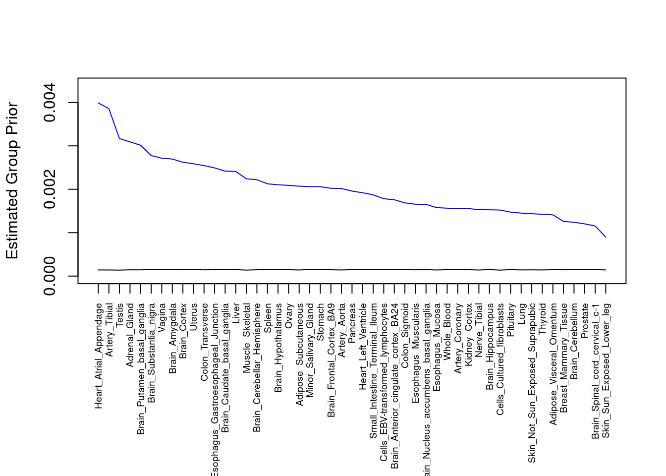
####################
#plot estimated group prior variance

par(mar=c(10.1, 4.1, 4.1, 2.1))

plot(output$prior_var_g, type="l", ylim=c(0, max(output$prior_var_g, output$prior_var_s)*1.1),
     xlab="", ylab="Estimated Group Prior Variance", xaxt = "n", col="blue")
lines(output$prior_var_s)

axis(1, at = 1:nrow(output),
     labels = output$weight,
     las=2,
     cex.axis=0.6)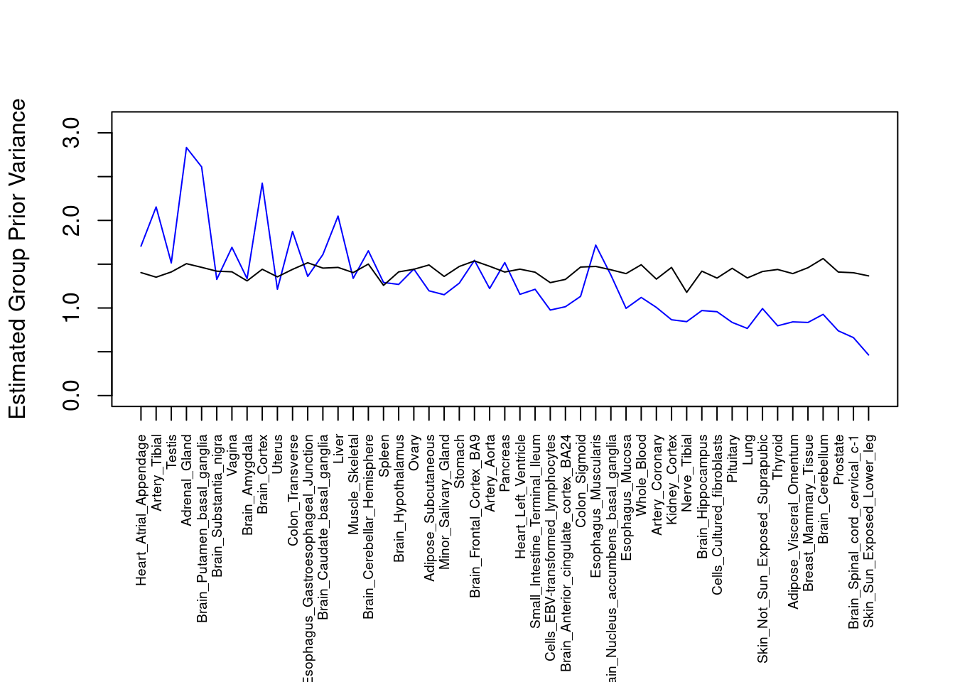
####################
#plot PVE

output <- output[order(-output$pve_g),]

par(mar=c(10.1, 4.1, 4.1, 2.1))

#plot(output$pve_g, type="l", ylim=c(0, max(output$pve_g, output$pve_s)*1.1),
plot(output$pve_g, type="l", ylim=c(0, max(output$pve_g+output$pve_s)*1.1),
     xlab="", ylab="Estimated PVE", xaxt = "n", col="blue")
lines(output$pve_s)
lines(output$pve_g+output$pve_s, lty=2)

axis(1, at = 1:nrow(output),
     labels = output$weight,
     las=2,
     cex.axis=0.6)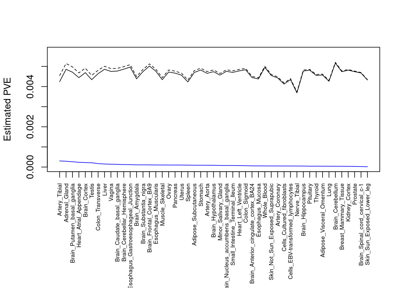
Number of cTWAS and TWAS genes
cTWAS genes are the set of genes with PIP>0.8 in any tissue. TWAS genes are the set of genes with significant z score (Bonferroni within tissue) in any tissue.
#plot number of significant cTWAS and TWAS genes in each tissue
plot(output$n_ctwas, output$n_twas, xlab="Number of cTWAS Genes", ylab="Number of TWAS Genes")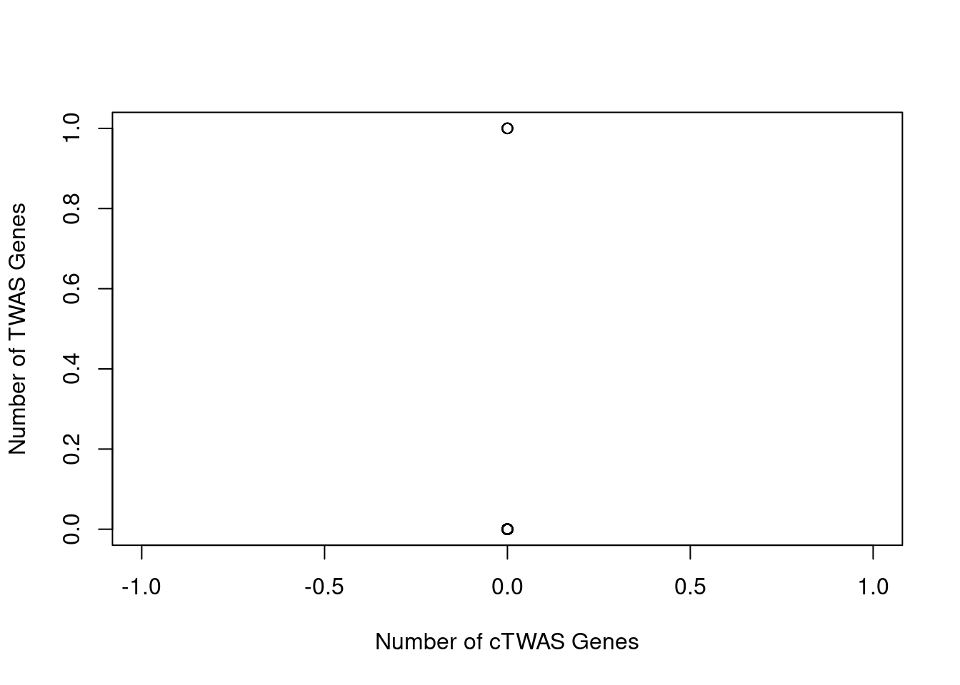
#number of ctwas_genes
ctwas_genes <- unique(unlist(lapply(df, function(x){x$ctwas})))
length(ctwas_genes)
[1] 0#number of twas_genes
twas_genes <- unique(unlist(lapply(df, function(x){x$twas})))
length(twas_genes)[1] 4
sessionInfo()R version 3.6.1 (2019-07-05)
Platform: x86_64-pc-linux-gnu (64-bit)
Running under: Scientific Linux 7.4 (Nitrogen)
Matrix products: default
BLAS/LAPACK: /software/openblas-0.2.19-el7-x86_64/lib/libopenblas_haswellp-r0.2.19.so
locale:
[1] LC_CTYPE=en_US.UTF-8 LC_NUMERIC=C
[3] LC_TIME=en_US.UTF-8 LC_COLLATE=en_US.UTF-8
[5] LC_MONETARY=en_US.UTF-8 LC_MESSAGES=en_US.UTF-8
[7] LC_PAPER=en_US.UTF-8 LC_NAME=C
[9] LC_ADDRESS=C LC_TELEPHONE=C
[11] LC_MEASUREMENT=en_US.UTF-8 LC_IDENTIFICATION=C
attached base packages:
[1] stats graphics grDevices utils datasets methods base
loaded via a namespace (and not attached):
[1] workflowr_1.6.2 Rcpp_1.0.6 rprojroot_2.0.2 digest_0.6.20
[5] later_0.8.0 R6_2.5.0 git2r_0.26.1 magrittr_2.0.1
[9] evaluate_0.14 stringi_1.4.3 fs_1.3.1 promises_1.0.1
[13] whisker_0.3-2 rmarkdown_1.13 tools_3.6.1 stringr_1.4.0
[17] glue_1.4.2 httpuv_1.5.1 xfun_0.8 yaml_2.2.0
[21] compiler_3.6.1 htmltools_0.3.6 knitr_1.23