Diagnoses - main ICD10: I48 Atrial fibrillation and flutter - Heart_Left_Ventricle
wesleycrouse
2021-09-7
Last updated: 2021-09-13
Checks: 7 0
Knit directory: ctwas_applied/
This reproducible R Markdown analysis was created with workflowr (version 1.6.2). The Checks tab describes the reproducibility checks that were applied when the results were created. The Past versions tab lists the development history.
Great! Since the R Markdown file has been committed to the Git repository, you know the exact version of the code that produced these results.
Great job! The global environment was empty. Objects defined in the global environment can affect the analysis in your R Markdown file in unknown ways. For reproduciblity it’s best to always run the code in an empty environment.
The command set.seed(20210726) was run prior to running the code in the R Markdown file. Setting a seed ensures that any results that rely on randomness, e.g. subsampling or permutations, are reproducible.
Great job! Recording the operating system, R version, and package versions is critical for reproducibility.
Nice! There were no cached chunks for this analysis, so you can be confident that you successfully produced the results during this run.
Great job! Using relative paths to the files within your workflowr project makes it easier to run your code on other machines.
Great! You are using Git for version control. Tracking code development and connecting the code version to the results is critical for reproducibility.
The results in this page were generated with repository version 72c8ef7. See the Past versions tab to see a history of the changes made to the R Markdown and HTML files.
Note that you need to be careful to ensure that all relevant files for the analysis have been committed to Git prior to generating the results (you can use wflow_publish or wflow_git_commit). workflowr only checks the R Markdown file, but you know if there are other scripts or data files that it depends on. Below is the status of the Git repository when the results were generated:
working directory clean
Note that any generated files, e.g. HTML, png, CSS, etc., are not included in this status report because it is ok for generated content to have uncommitted changes.
These are the previous versions of the repository in which changes were made to the R Markdown (analysis/ukb-a-536_Heart_Left_Ventricle_known.Rmd) and HTML (docs/ukb-a-536_Heart_Left_Ventricle_known.html) files. If you’ve configured a remote Git repository (see ?wflow_git_remote), click on the hyperlinks in the table below to view the files as they were in that past version.
| File | Version | Author | Date | Message |
|---|---|---|---|---|
| html | 7e22565 | wesleycrouse | 2021-09-13 | updating reports |
| Rmd | 3a7fbc1 | wesleycrouse | 2021-09-08 | generating reports for known annotations |
| html | 3a7fbc1 | wesleycrouse | 2021-09-08 | generating reports for known annotations |
| Rmd | cbf7408 | wesleycrouse | 2021-09-08 | adding enrichment to reports |
Overview
These are the results of a ctwas analysis of the UK Biobank trait Diagnoses - main ICD10: I48 Atrial fibrillation and flutter using Heart_Left_Ventricle gene weights.
The GWAS was conducted by the Neale Lab, and the biomarker traits we analyzed are discussed here. Summary statistics were obtained from IEU OpenGWAS using GWAS ID: ukb-a-536. Results were obtained from from IEU rather than Neale Lab because they are in a standardard format (GWAS VCF). Note that 3 of the 34 biomarker traits were not available from IEU and were excluded from analysis.
The weights are mashr GTEx v8 models on Heart_Left_Ventricle eQTL obtained from PredictDB. We performed a full harmonization of the variants, including recovering strand ambiguous variants. This procedure is discussed in a separate document. (TO-DO: add report that describes harmonization)
LD matrices were computed from a 10% subset of Neale lab subjects. Subjects were matched using the plate and well information from genotyping. We included only biallelic variants with MAF>0.01 in the original Neale Lab GWAS. (TO-DO: add more details [number of subjects, variants, etc])
Weight QC
TO-DO: add enhanced QC reporting (total number of weights, why each variant was missing for all genes)
qclist_all <- list()

qc_files <- paste0(results_dir, "/", list.files(results_dir, pattern="exprqc.Rd"))

for (i in 1:length(qc_files)){
  load(qc_files[i])
  chr <- unlist(strsplit(rev(unlist(strsplit(qc_files[i], "_")))[1], "[.]"))[1]
  qclist_all[[chr]] <- cbind(do.call(rbind, lapply(qclist,unlist)), as.numeric(substring(chr,4)))
}

qclist_all <- data.frame(do.call(rbind, qclist_all))
colnames(qclist_all)[ncol(qclist_all)] <- "chr"

rm(qclist, wgtlist, z_gene_chr)

#number of imputed weights
nrow(qclist_all)
[1] 10971#number of imputed weights by chromosome
table(qclist_all$chr)
   1    2    3    4    5    6    7    8    9   10   11   12   13   14   15
1078  769  621  445  494  650  544  404  412  451  645  591  199  362  370
  16   17   18   19   20   21   22
 529  681  157  850  330  119  270
#proportion of imputed weights without missing variants
mean(qclist_all$nmiss==0)[1] 0.7405888Load ctwas results
#load ctwas results
ctwas_res <- data.table::fread(paste0(results_dir, "/", analysis_id, "_ctwas.susieIrss.txt"))

#make unique identifier for regions
ctwas_res$region_tag <- paste(ctwas_res$region_tag1, ctwas_res$region_tag2, sep="_")

#load z scores for SNPs and collect sample size
load(paste0(results_dir, "/", analysis_id, "_expr_z_snp.Rd"))

sample_size <- z_snp$ss
sample_size <- as.numeric(names(which.max(table(sample_size))))

#compute PVE for each gene/SNP
ctwas_res$PVE = ctwas_res$susie_pip*ctwas_res$mu2/sample_size

#separate gene and SNP results
ctwas_gene_res <- ctwas_res[ctwas_res$type == "gene", ]
ctwas_gene_res <- data.frame(ctwas_gene_res)
ctwas_snp_res <- ctwas_res[ctwas_res$type == "SNP", ]
ctwas_snp_res <- data.frame(ctwas_snp_res)

#add gene information to results
sqlite <- RSQLite::dbDriver("SQLite")
db = RSQLite::dbConnect(sqlite, paste0("/project2/compbio/predictdb/mashr_models/mashr_", weight, ".db"))
query <- function(...) RSQLite::dbGetQuery(db, ...)
gene_info <- query("select gene, genename from extra")
gene_info <- query("select gene, genename, gene_type from extra")
RSQLite::dbDisconnect(db)

ctwas_gene_res <- cbind(ctwas_gene_res, gene_info[sapply(ctwas_gene_res$id, match, gene_info$gene), c("genename", "gene_type")])

#add z scores to results
load(paste0(results_dir, "/", analysis_id, "_expr_z_gene.Rd"))
ctwas_gene_res$z <- z_gene[ctwas_gene_res$id,]$z

z_snp <- z_snp[z_snp$id %in% ctwas_snp_res$id,]
ctwas_snp_res$z <- z_snp$z[match(ctwas_snp_res$id, z_snp$id)]

#formatting and rounding for tables
ctwas_gene_res$z <- round(ctwas_gene_res$z,2)
ctwas_snp_res$z <- round(ctwas_snp_res$z,2)
ctwas_gene_res$susie_pip <- round(ctwas_gene_res$susie_pip,3)
ctwas_snp_res$susie_pip <- round(ctwas_snp_res$susie_pip,3)
ctwas_gene_res$mu2 <- round(ctwas_gene_res$mu2,2)
ctwas_snp_res$mu2 <- round(ctwas_snp_res$mu2,2)
ctwas_gene_res$PVE <- signif(ctwas_gene_res$PVE, 2)
ctwas_snp_res$PVE <- signif(ctwas_snp_res$PVE, 2)

#merge gene and snp results with added information
ctwas_snp_res$genename=NA
ctwas_snp_res$gene_type=NA

ctwas_res <- rbind(ctwas_gene_res,
                   ctwas_snp_res[,colnames(ctwas_gene_res)])

#store columns to report
report_cols <- colnames(ctwas_gene_res)[!(colnames(ctwas_gene_res) %in% c("type", "region_tag1", "region_tag2", "cs_index", "gene_type", "z_flag", "id", "chrom", "pos"))]
first_cols <- c("genename", "region_tag")
report_cols <- c(first_cols, report_cols[!(report_cols %in% first_cols)])

report_cols_snps <- c("id", report_cols[-1])

#get number of SNPs from s1 results; adjust for thin
ctwas_res_s1 <- data.table::fread(paste0(results_dir, "/", analysis_id, "_ctwas.s1.susieIrss.txt"))
n_snps <- sum(ctwas_res_s1$type=="SNP")/thin
rm(ctwas_res_s1)
Check convergence of parameters
library(ggplot2)
library(cowplot)
********************************************************Note: As of version 1.0.0, cowplot does not change the default ggplot2 theme anymore. To recover the previous behavior, execute:
theme_set(theme_cowplot())********************************************************load(paste0(results_dir, "/", analysis_id, "_ctwas.s2.susieIrssres.Rd"))
df <- data.frame(niter = rep(1:ncol(group_prior_rec), 2),
value = c(group_prior_rec[1,], group_prior_rec[2,]),
group = rep(c("Gene", "SNP"), each = ncol(group_prior_rec)))
df$group <- as.factor(df$group)
df$value[df$group=="SNP"] <- df$value[df$group=="SNP"]*thin #adjust parameter to account for thin argument
p_pi <- ggplot(df, aes(x=niter, y=value, group=group)) +
geom_line(aes(color=group)) +
geom_point(aes(color=group)) +
xlab("Iteration") + ylab(bquote(pi)) +
ggtitle("Prior mean") +
theme_cowplot()
df <- data.frame(niter = rep(1:ncol(group_prior_var_rec), 2),
value = c(group_prior_var_rec[1,], group_prior_var_rec[2,]),
group = rep(c("Gene", "SNP"), each = ncol(group_prior_var_rec)))
df$group <- as.factor(df$group)
p_sigma2 <- ggplot(df, aes(x=niter, y=value, group=group)) +
geom_line(aes(color=group)) +
geom_point(aes(color=group)) +
xlab("Iteration") + ylab(bquote(sigma^2)) +
ggtitle("Prior variance") +
theme_cowplot()
plot_grid(p_pi, p_sigma2)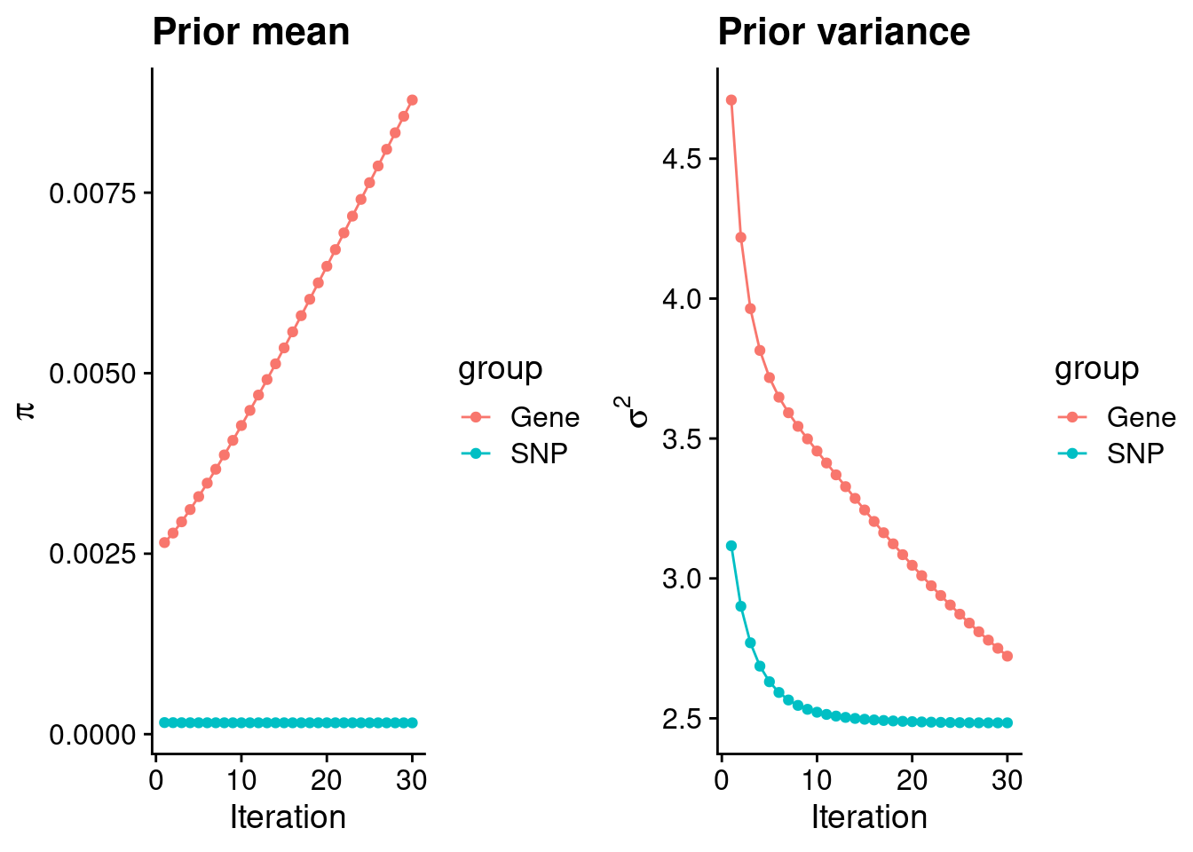
| Version | Author | Date |
|---|---|---|
| 3a7fbc1 | wesleycrouse | 2021-09-08 |
#estimated group prior
estimated_group_prior <- group_prior_rec[,ncol(group_prior_rec)]
names(estimated_group_prior) <- c("gene", "snp")
estimated_group_prior["snp"] <- estimated_group_prior["snp"]*thin #adjust parameter to account for thin argument
print(estimated_group_prior)
gene snp
0.0087835822 0.0001568083 #estimated group prior variance
estimated_group_prior_var <- group_prior_var_rec[,ncol(group_prior_var_rec)]
names(estimated_group_prior_var) <- c("gene", "snp")
print(estimated_group_prior_var) gene snp
2.722269 2.483925 #report sample size
print(sample_size)[1] 337199#report group size
group_size <- c(nrow(ctwas_gene_res), n_snps)
print(group_size)[1] 10971 7535010#estimated group PVE
estimated_group_pve <- estimated_group_prior_var*estimated_group_prior*group_size/sample_size #check PVE calculation
names(estimated_group_pve) <- c("gene", "snp")
print(estimated_group_pve) gene snp
0.0007779696 0.0087037244 #compare sum(PIP*mu2/sample_size) with above PVE calculation
c(sum(ctwas_gene_res$PVE),sum(ctwas_snp_res$PVE))[1] 0.00970027 0.14034857Genes with highest PIPs
#distribution of PIPs
hist(ctwas_gene_res$susie_pip, xlim=c(0,1), main="Distribution of Gene PIPs")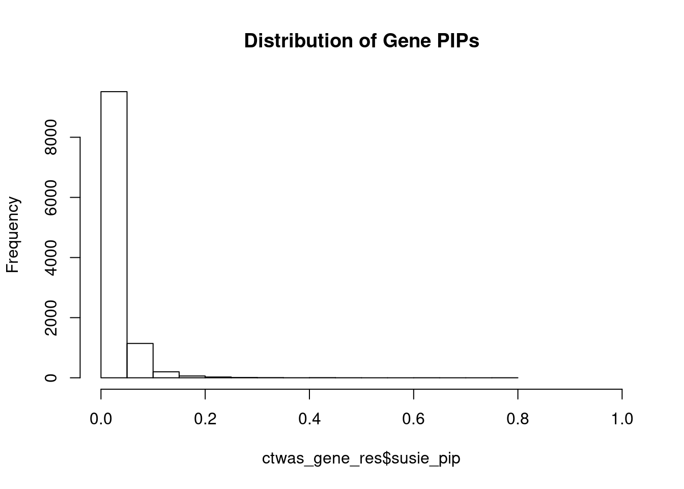
| Version | Author | Date |
|---|---|---|
| 3a7fbc1 | wesleycrouse | 2021-09-08 |
#genes with PIP>0.8 or 20 highest PIPs
head(ctwas_gene_res[order(-ctwas_gene_res$susie_pip),report_cols], max(sum(ctwas_gene_res$susie_pip>0.8), 20))
genename region_tag susie_pip mu2 PVE z
3725 SSPN 12_18 0.777 23.82 5.5e-05 -5.47
3147 WIPF1 2_105 0.628 23.59 4.4e-05 4.81
2401 PITX3 10_65 0.497 22.47 3.3e-05 -5.35
2380 SEC23IP 10_74 0.452 27.22 3.7e-05 -4.14
3169 PRRX1 1_84 0.445 26.36 3.5e-05 5.30
7794 KDM1B 6_14 0.436 20.51 2.7e-05 -4.75
3876 DEK 6_14 0.424 20.53 2.6e-05 -4.73
1374 SLC22A17 14_3 0.416 31.18 3.8e-05 -4.78
2987 GNB4 3_110 0.413 26.30 3.2e-05 -3.87
503 TBC1D22A 22_21 0.384 26.57 3.0e-05 3.91
7205 SRSF2 17_43 0.352 25.50 2.7e-05 -3.60
6373 NOCT 4_92 0.342 24.28 2.5e-05 3.54
7939 FBN1 15_19 0.328 24.15 2.3e-05 3.44
7567 LIPH 3_114 0.313 23.79 2.2e-05 3.85
9712 COPG1 3_80 0.312 23.02 2.1e-05 -3.66
844 SCARB1 12_76 0.308 23.23 2.1e-05 3.69
1298 LTBP4 19_28 0.304 23.51 2.1e-05 -3.38
1031 DDX43 6_51 0.273 21.92 1.8e-05 3.45
9646 OXTR 3_7 0.271 22.54 1.8e-05 3.12
7278 C1orf123 1_33 0.270 21.86 1.8e-05 -3.37Genes with largest effect sizes
#plot PIP vs effect size
plot(ctwas_gene_res$susie_pip, ctwas_gene_res$mu2, xlab="PIP", ylab="mu^2", main="Gene PIPs vs Effect Size")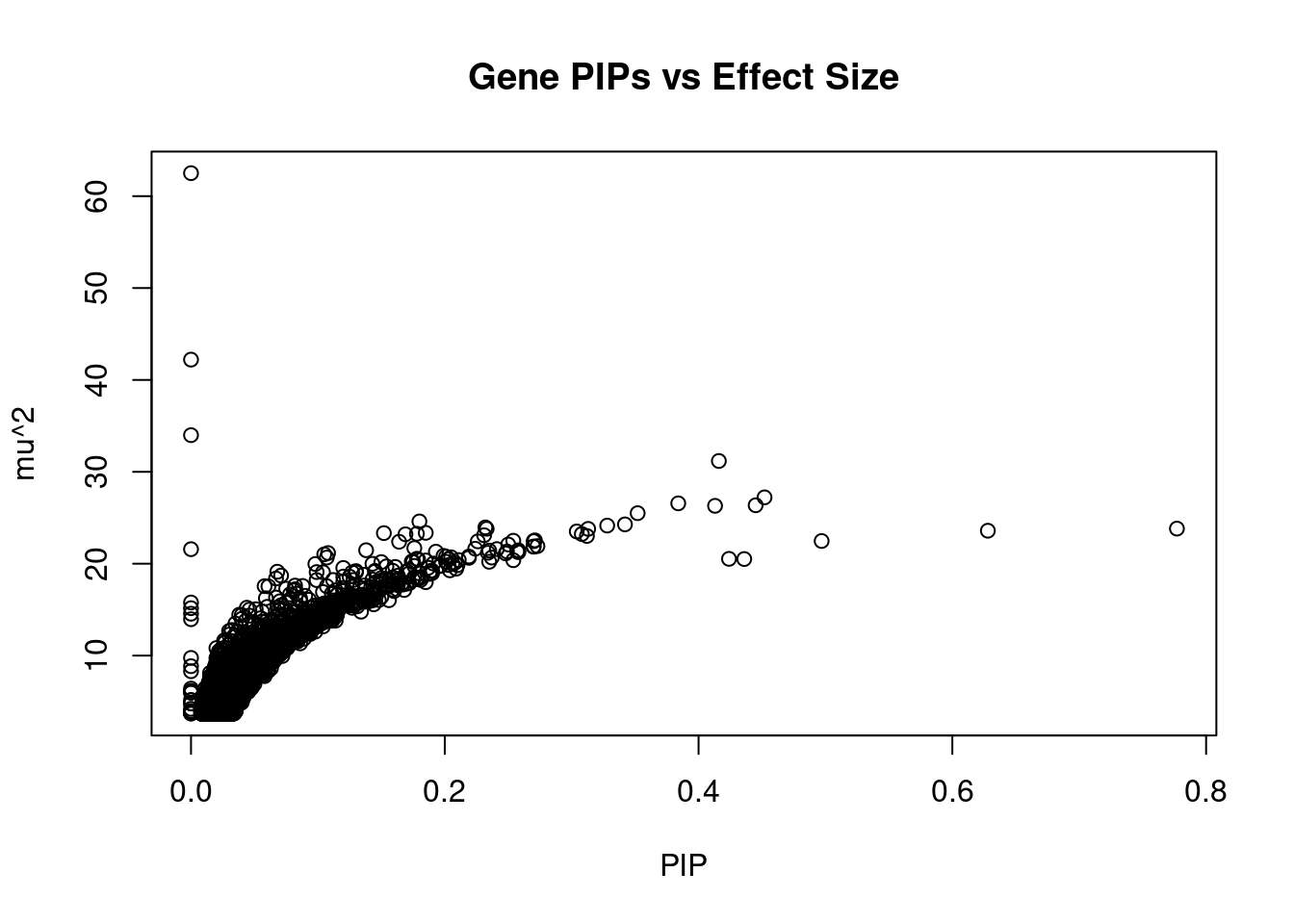
| Version | Author | Date |
|---|---|---|
| 3a7fbc1 | wesleycrouse | 2021-09-08 |
#genes with 20 largest effect sizes
head(ctwas_gene_res[order(-ctwas_gene_res$mu2),report_cols],20)
genename region_tag susie_pip mu2 PVE z
9455 STX19 3_59 0.000 62.50 4.1e-14 0.17
9450 NSUN3 3_59 0.000 42.21 9.3e-14 -1.48
9987 PROS1 3_59 0.000 33.99 7.7e-14 -2.06
1374 SLC22A17 14_3 0.416 31.18 3.8e-05 -4.78
2380 SEC23IP 10_74 0.452 27.22 3.7e-05 -4.14
503 TBC1D22A 22_21 0.384 26.57 3.0e-05 3.91
3169 PRRX1 1_84 0.445 26.36 3.5e-05 5.30
2987 GNB4 3_110 0.413 26.30 3.2e-05 -3.87
7205 SRSF2 17_43 0.352 25.50 2.7e-05 -3.60
7445 DCST2 1_76 0.180 24.60 1.3e-05 -4.49
6373 NOCT 4_92 0.342 24.28 2.5e-05 3.54
7939 FBN1 15_19 0.328 24.15 2.3e-05 3.44
9511 ZNF664 12_75 0.232 23.95 1.7e-05 3.65
3725 SSPN 12_18 0.777 23.82 5.5e-05 -5.47
12085 MIR4458HG 5_8 0.233 23.80 1.6e-05 -3.25
7567 LIPH 3_114 0.313 23.79 2.2e-05 3.85
3147 WIPF1 2_105 0.628 23.59 4.4e-05 4.81
1298 LTBP4 19_28 0.304 23.51 2.1e-05 -3.38
4518 EIF5A 17_7 0.185 23.36 1.3e-05 -3.45
11057 ZNF525 19_36 0.152 23.33 1.0e-05 2.97Genes with highest PVE
#genes with 20 highest pve
head(ctwas_gene_res[order(-ctwas_gene_res$PVE),report_cols],20)
genename region_tag susie_pip mu2 PVE z
3725 SSPN 12_18 0.777 23.82 5.5e-05 -5.47
3147 WIPF1 2_105 0.628 23.59 4.4e-05 4.81
1374 SLC22A17 14_3 0.416 31.18 3.8e-05 -4.78
2380 SEC23IP 10_74 0.452 27.22 3.7e-05 -4.14
3169 PRRX1 1_84 0.445 26.36 3.5e-05 5.30
2401 PITX3 10_65 0.497 22.47 3.3e-05 -5.35
2987 GNB4 3_110 0.413 26.30 3.2e-05 -3.87
503 TBC1D22A 22_21 0.384 26.57 3.0e-05 3.91
7794 KDM1B 6_14 0.436 20.51 2.7e-05 -4.75
7205 SRSF2 17_43 0.352 25.50 2.7e-05 -3.60
3876 DEK 6_14 0.424 20.53 2.6e-05 -4.73
6373 NOCT 4_92 0.342 24.28 2.5e-05 3.54
7939 FBN1 15_19 0.328 24.15 2.3e-05 3.44
7567 LIPH 3_114 0.313 23.79 2.2e-05 3.85
9712 COPG1 3_80 0.312 23.02 2.1e-05 -3.66
844 SCARB1 12_76 0.308 23.23 2.1e-05 3.69
1298 LTBP4 19_28 0.304 23.51 2.1e-05 -3.38
7278 C1orf123 1_33 0.270 21.86 1.8e-05 -3.37
9646 OXTR 3_7 0.271 22.54 1.8e-05 3.12
10102 GPRIN3 4_60 0.270 22.45 1.8e-05 3.17Genes with largest z scores
#genes with 20 largest z scores
head(ctwas_gene_res[order(-abs(ctwas_gene_res$z)),report_cols],20)
genename region_tag susie_pip mu2 PVE z
3725 SSPN 12_18 0.777 23.82 5.5e-05 -5.47
2401 PITX3 10_65 0.497 22.47 3.3e-05 -5.35
3169 PRRX1 1_84 0.445 26.36 3.5e-05 5.30
3147 WIPF1 2_105 0.628 23.59 4.4e-05 4.81
12761 RP1-79C4.4 1_84 0.231 23.10 1.6e-05 4.80
1374 SLC22A17 14_3 0.416 31.18 3.8e-05 -4.78
7794 KDM1B 6_14 0.436 20.51 2.7e-05 -4.75
3876 DEK 6_14 0.424 20.53 2.6e-05 -4.73
7445 DCST2 1_76 0.180 24.60 1.3e-05 -4.49
7134 ZBTB7B 1_76 0.046 15.00 2.0e-06 4.18
2380 SEC23IP 10_74 0.452 27.22 3.7e-05 -4.14
503 TBC1D22A 22_21 0.384 26.57 3.0e-05 3.91
2554 SLC2A9 4_11 0.254 22.50 1.7e-05 -3.88
2987 GNB4 3_110 0.413 26.30 3.2e-05 -3.87
7567 LIPH 3_114 0.313 23.79 2.2e-05 3.85
6811 FBXO32 8_80 0.178 23.26 1.2e-05 -3.80
7930 CMTM5 14_3 0.138 21.47 8.8e-06 -3.80
7381 MAIP1 2_118 0.127 19.06 7.2e-06 -3.71
844 SCARB1 12_76 0.308 23.23 2.1e-05 3.69
3052 STAM2 2_91 0.241 21.59 1.5e-05 3.68Comparing z scores and PIPs
#set nominal signifiance threshold for z scores
alpha <- 0.05

#bonferroni adjusted threshold for z scores
sig_thresh <- qnorm(1-(alpha/nrow(ctwas_gene_res)/2), lower=T)

#Q-Q plot for z scores
obs_z <- ctwas_gene_res$z[order(ctwas_gene_res$z)]
exp_z <- qnorm((1:nrow(ctwas_gene_res))/nrow(ctwas_gene_res))

plot(exp_z, obs_z, xlab="Expected z", ylab="Observed z", main="Gene z score Q-Q plot")
abline(a=0,b=1)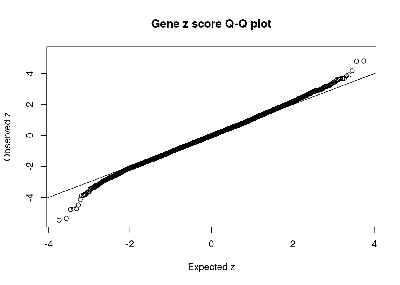
| Version | Author | Date |
|---|---|---|
| 3a7fbc1 | wesleycrouse | 2021-09-08 |
#plot z score vs PIP
plot(abs(ctwas_gene_res$z), ctwas_gene_res$susie_pip, xlab="abs(z)", ylab="PIP")
abline(v=sig_thresh, col="red", lty=2)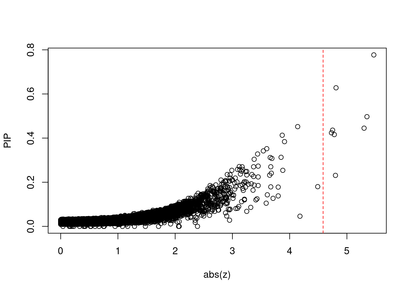
| Version | Author | Date |
|---|---|---|
| 3a7fbc1 | wesleycrouse | 2021-09-08 |
#proportion of significant z scores
mean(abs(ctwas_gene_res$z) > sig_thresh)
[1] 0.0007291952#genes with most significant z scores
head(ctwas_gene_res[order(-abs(ctwas_gene_res$z)),report_cols],20) genename region_tag susie_pip mu2 PVE z
3725 SSPN 12_18 0.777 23.82 5.5e-05 -5.47
2401 PITX3 10_65 0.497 22.47 3.3e-05 -5.35
3169 PRRX1 1_84 0.445 26.36 3.5e-05 5.30
3147 WIPF1 2_105 0.628 23.59 4.4e-05 4.81
12761 RP1-79C4.4 1_84 0.231 23.10 1.6e-05 4.80
1374 SLC22A17 14_3 0.416 31.18 3.8e-05 -4.78
7794 KDM1B 6_14 0.436 20.51 2.7e-05 -4.75
3876 DEK 6_14 0.424 20.53 2.6e-05 -4.73
7445 DCST2 1_76 0.180 24.60 1.3e-05 -4.49
7134 ZBTB7B 1_76 0.046 15.00 2.0e-06 4.18
2380 SEC23IP 10_74 0.452 27.22 3.7e-05 -4.14
503 TBC1D22A 22_21 0.384 26.57 3.0e-05 3.91
2554 SLC2A9 4_11 0.254 22.50 1.7e-05 -3.88
2987 GNB4 3_110 0.413 26.30 3.2e-05 -3.87
7567 LIPH 3_114 0.313 23.79 2.2e-05 3.85
6811 FBXO32 8_80 0.178 23.26 1.2e-05 -3.80
7930 CMTM5 14_3 0.138 21.47 8.8e-06 -3.80
7381 MAIP1 2_118 0.127 19.06 7.2e-06 -3.71
844 SCARB1 12_76 0.308 23.23 2.1e-05 3.69
3052 STAM2 2_91 0.241 21.59 1.5e-05 3.68Locus plots for genes and SNPs
ctwas_gene_res_sortz <- ctwas_gene_res[order(-abs(ctwas_gene_res$z)),]

n_plots <- 5
for (region_tag_plot in head(unique(ctwas_gene_res_sortz$region_tag), n_plots)){
  ctwas_res_region <-  ctwas_res[ctwas_res$region_tag==region_tag_plot,]
  start <- min(ctwas_res_region$pos)
  end <- max(ctwas_res_region$pos)

  ctwas_res_region <- ctwas_res_region[order(ctwas_res_region$pos),]
  ctwas_res_region_gene <- ctwas_res_region[ctwas_res_region$type=="gene",]
  ctwas_res_region_snp <- ctwas_res_region[ctwas_res_region$type=="SNP",]

  #region name
  print(paste0("Region: ", region_tag_plot))

  #table of genes in region
  print(ctwas_res_region_gene[,report_cols])

  par(mfrow=c(4,1))

  #gene z scores
  plot(ctwas_res_region_gene$pos, abs(ctwas_res_region_gene$z), xlab="Position", ylab="abs(gene_z)", xlim=c(start,end),
   ylim=c(0,max(sig_thresh, abs(ctwas_res_region_gene$z))),
   main=paste0("Region: ", region_tag_plot))
  abline(h=sig_thresh,col="red",lty=2)

  #significance threshold for SNPs
  alpha_snp <- 5*10^(-8)
  sig_thresh_snp <- qnorm(1-alpha_snp/2, lower=T)

  #snp z scores
  plot(ctwas_res_region_snp$pos, abs(ctwas_res_region_snp$z), xlab="Position", ylab="abs(snp_z)",xlim=c(start,end),
   ylim=c(0,max(sig_thresh_snp, max(abs(ctwas_res_region_snp$z)))))
  abline(h=sig_thresh_snp,col="purple",lty=2)

  #gene pips
  plot(ctwas_res_region_gene$pos, ctwas_res_region_gene$susie_pip, xlab="Position", ylab="Gene PIP", xlim=c(start,end), ylim=c(0,1))
  abline(h=0.8,col="blue",lty=2)

  #snp pips
  plot(ctwas_res_region_snp$pos, ctwas_res_region_snp$susie_pip, xlab="Position", ylab="SNP PIP", xlim=c(start,end), ylim=c(0,1))
  abline(h=0.8,col="blue",lty=2)
}
[1] "Region: 12_18"
genename region_tag susie_pip mu2 PVE z
13136 RP11-707G18.1 12_18 0.027 9.72 7.9e-07 -1.67
3723 RASSF8 12_18 0.082 17.62 4.3e-06 -2.57
3724 BHLHE41 12_18 0.068 19.13 3.9e-06 3.25
3725 SSPN 12_18 0.777 23.82 5.5e-05 -5.47
3726 ITPR2 12_18 0.013 4.17 1.6e-07 -0.53
600 INTS13 12_18 0.025 9.22 7.0e-07 -1.53
2749 FGFR1OP2 12_18 0.025 9.22 7.0e-07 1.53
601 TM7SF3 12_18 0.012 3.86 1.4e-07 -0.34
13030 RP11-582E3.6 12_18 0.016 5.79 2.7e-07 1.06
6540 MED21 12_18 0.021 7.97 5.0e-07 -1.43
11318 STK38L 12_18 0.014 4.70 1.9e-07 -0.65
333 ARNTL2 12_18 0.060 15.31 2.7e-06 -2.11
7909 SMCO2 12_18 0.016 5.58 2.6e-07 0.89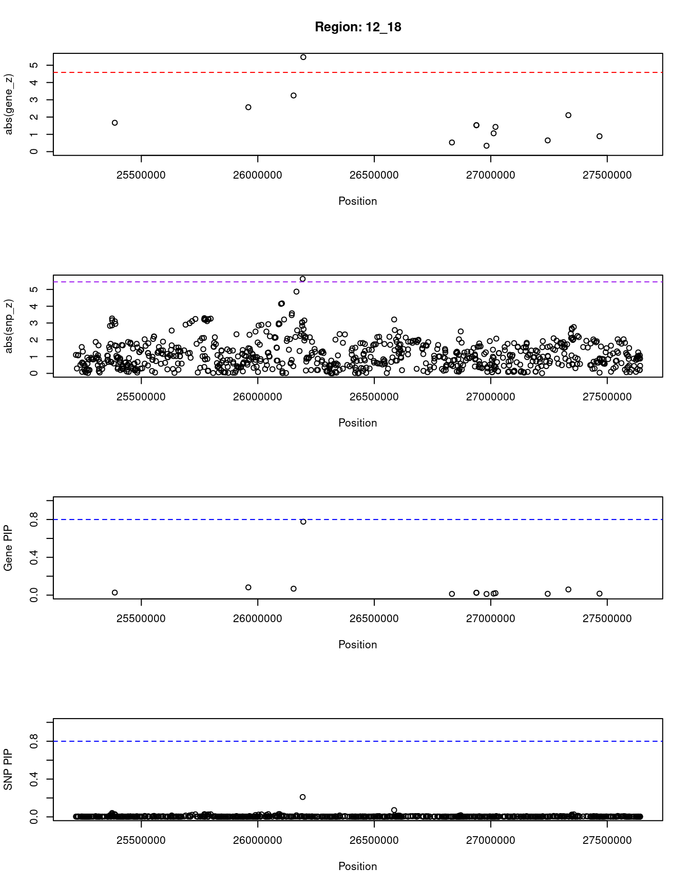
| Version | Author | Date |
|---|---|---|
| 3a7fbc1 | wesleycrouse | 2021-09-08 |
[1] "Region: 10_65"
      genename region_tag susie_pip   mu2     PVE     z
7945      BTRC      10_65     0.020  3.68 2.1e-07  0.12
7947      DPCD      10_65     0.020  3.79 2.2e-07 -0.40
2398     FBXW4      10_65     0.055 10.72 1.7e-06 -1.55
2399      NPM3      10_65     0.028  8.47 6.9e-07  2.35
10914    MGEA5      10_65     0.020  4.08 2.4e-07 -0.72
3509    KCNIP2      10_65     0.020  3.83 2.3e-07  0.25
3508  C10orf76      10_65     0.025  6.54 4.9e-07  1.81
10975     LDB1      10_65     0.023  4.65 3.1e-07  0.50
6247     PPRC1      10_65     0.032  7.75 7.3e-07  1.55
7953     NOLC1      10_65     0.024  5.69 4.0e-07  1.36
3496    ELOVL3      10_65     0.027  6.89 5.6e-07  1.57
2401     PITX3      10_65     0.497 22.47 3.3e-05 -5.35
2402      GBF1      10_65     0.040  9.26 1.1e-06  1.61
557        PSD      10_65     0.030  7.14 6.3e-07 -1.42
2405    FBXL15      10_65     0.020  4.10 2.4e-07  0.89
2406    CUEDC2      10_65     0.024  5.45 3.8e-07  1.12
5214   MFSD13A      10_65     0.021  4.16 2.6e-07  0.52
2407      SUFU      10_65     0.021  4.24 2.7e-07 -0.46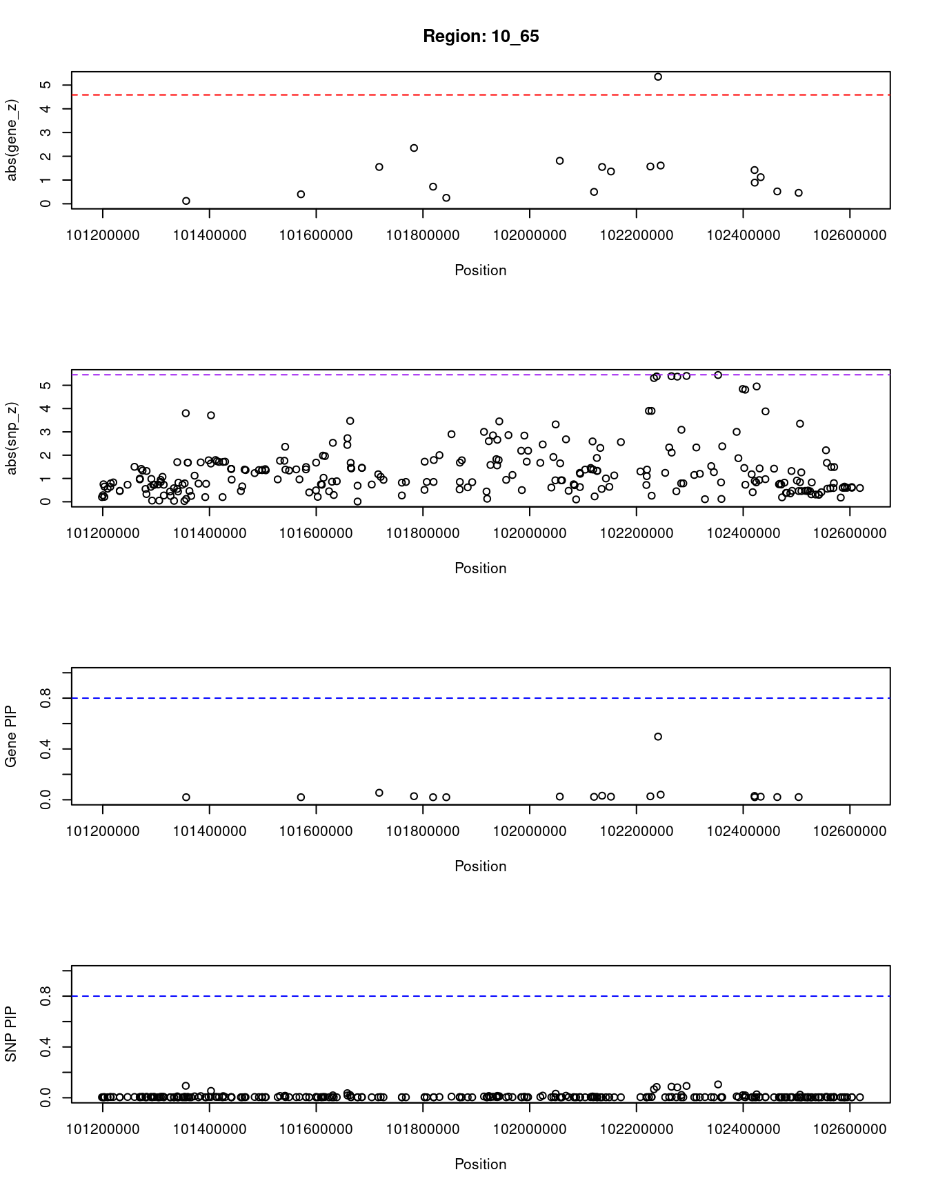
| Version | Author | Date |
|---|---|---|
| 3a7fbc1 | wesleycrouse | 2021-09-08 |
[1] "Region: 1_84"
        genename region_tag susie_pip   mu2     PVE     z
12761 RP1-79C4.4       1_84     0.231 23.10 1.6e-05  4.80
3169       PRRX1       1_84     0.445 26.36 3.5e-05  5.30
134         FMO3       1_84     0.015  3.82 1.7e-07  0.28
1412        FMO2       1_84     0.015  3.75 1.6e-07  0.28
195         FMO1       1_84     0.016  4.54 2.2e-07 -0.53
933         FMO4       1_84     0.014  3.67 1.6e-07  0.09
3311      PRRC2C       1_84     0.015  4.00 1.8e-07 -0.42
362         MYOC       1_84     0.015  3.77 1.6e-07 -0.23
174      METTL13       1_84     0.015  3.74 1.6e-07  0.24
10837       DNM3       1_84     0.020  6.02 3.6e-07 -0.94
4893        PIGC       1_84     0.015  3.71 1.6e-07  0.18
9656    C1orf105       1_84     0.014  3.67 1.6e-07 -0.04
1413        SUCO       1_84     0.016  4.51 2.2e-07  0.49
3315       FASLG       1_84     0.014  3.67 1.6e-07  0.06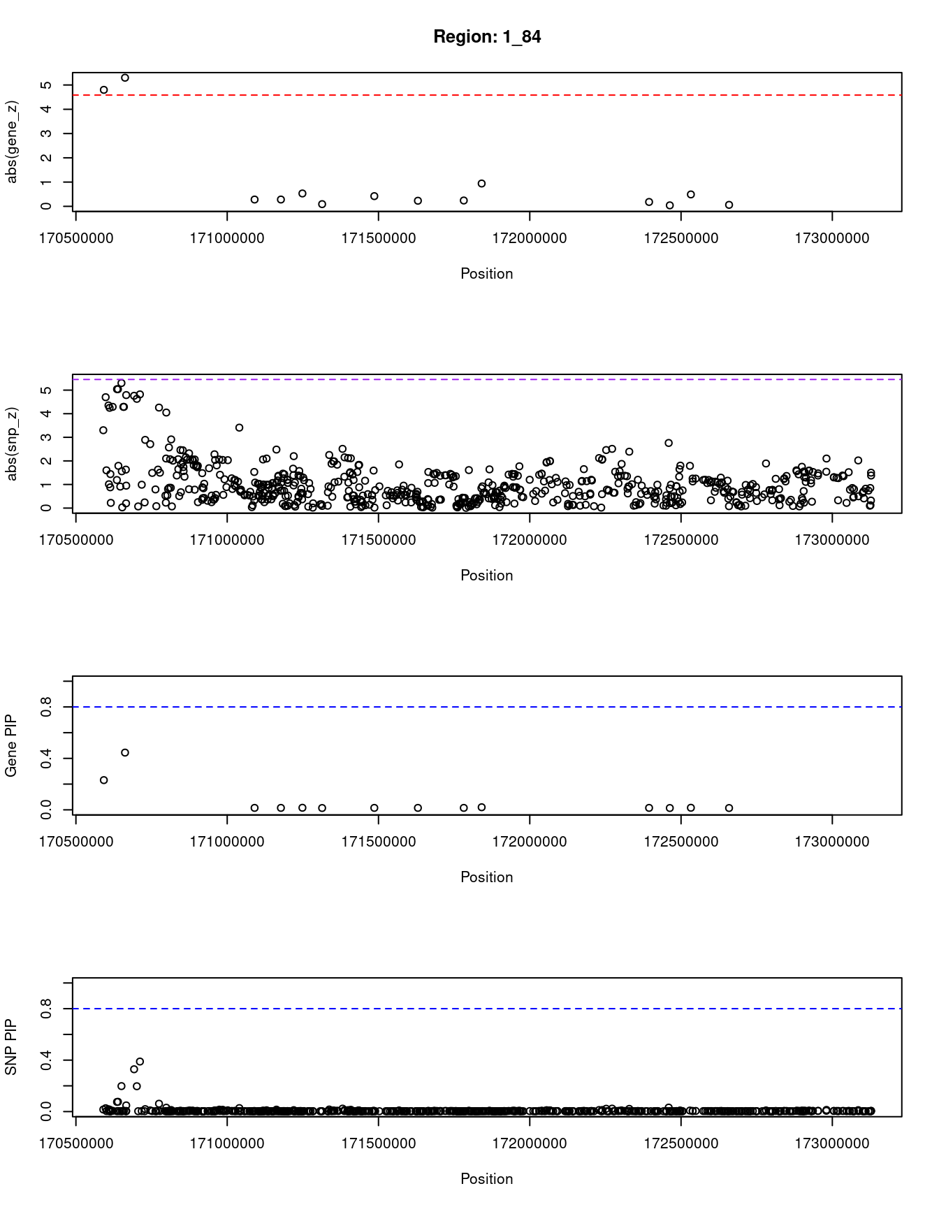
| Version | Author | Date |
|---|---|---|
| 3a7fbc1 | wesleycrouse | 2021-09-08 |
[1] "Region: 2_105"
           genename region_tag susie_pip   mu2     PVE     z
6480           PDK1      2_105     0.068 15.23 3.1e-06 -2.19
1348        MAP3K20      2_105     0.020  6.11 3.6e-07  0.96
5895          CDCA7      2_105     0.014  3.71 1.6e-07  0.20
8872            SP3      2_105     0.033 10.10 1.0e-06 -1.86
12726 RP11-394I13.2      2_105     0.038 11.02 1.2e-06 -2.00
5254           OLA1      2_105     0.082 17.22 4.2e-06  3.09
5892          SCRN3      2_105     0.078 16.66 3.9e-06  2.96
7442         GPR155      2_105     0.028  9.73 8.2e-07 -2.95
11646    AC010894.3      2_105     0.015  4.28 1.9e-07  1.46
3147          WIPF1      2_105     0.628 23.59 4.4e-05  4.81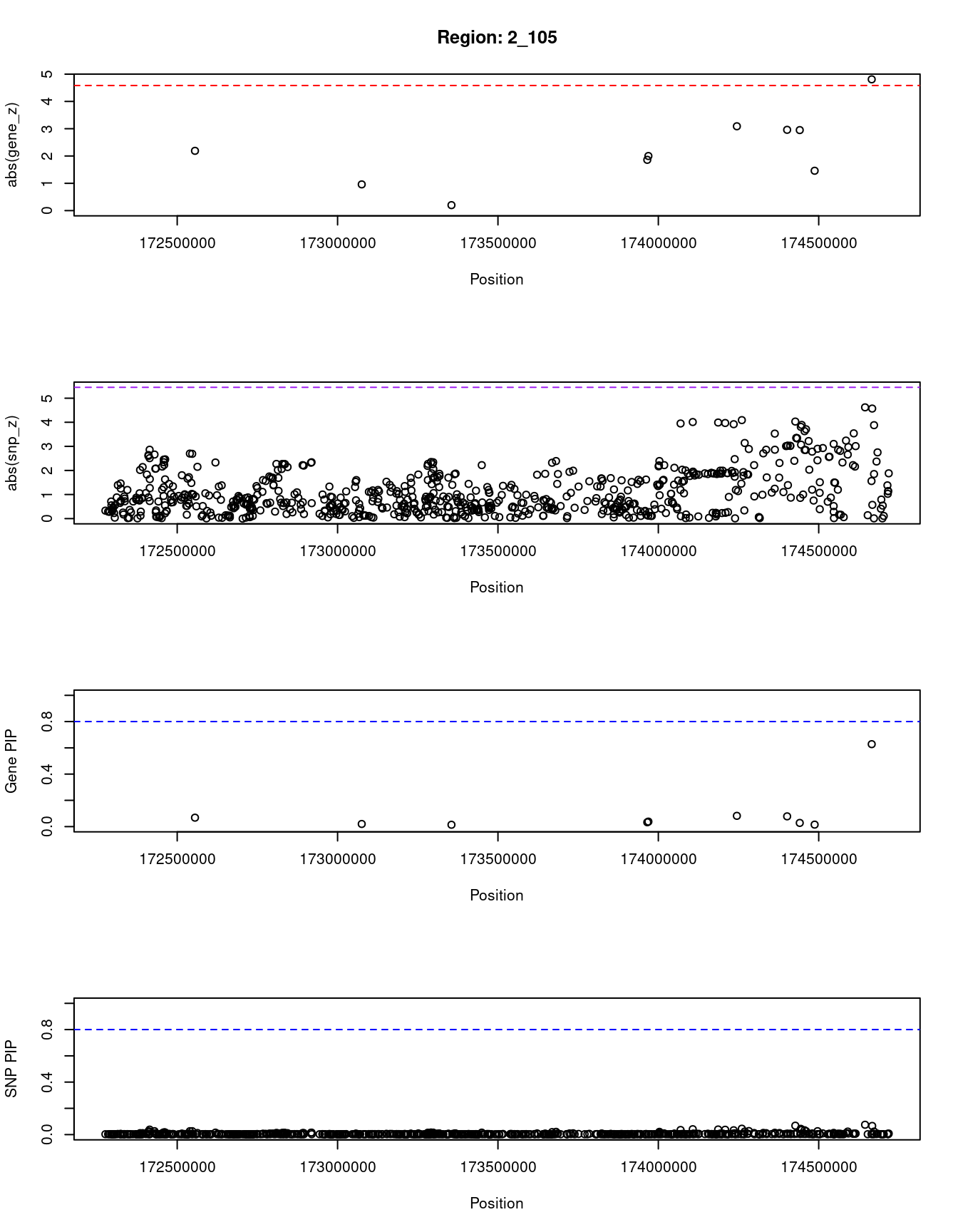
| Version | Author | Date |
|---|---|---|
| 3a7fbc1 | wesleycrouse | 2021-09-08 |
[1] "Region: 14_3"
           genename region_tag susie_pip   mu2     PVE     z
1629          ABHD4       14_3     0.014  4.82 2.1e-07 -0.68
6717          OXA1L       14_3     0.015  5.09 2.3e-07 -0.67
6843          MMP14       14_3     0.028  9.62 7.9e-07 -1.56
10731         LRP10       14_3     0.013  4.28 1.7e-07  0.52
1633          RBM23       14_3     0.012  3.66 1.3e-07 -0.06
1634          PRMT5       14_3     0.014  4.43 1.8e-07  0.55
1369          HAUS4       14_3     0.013  4.28 1.7e-07  0.44
4236          AJUBA       14_3     0.016  5.46 2.5e-07 -0.95
1679       C14orf93       14_3     0.012  3.66 1.3e-07 -0.07
1680          PSMB5       14_3     0.013  4.26 1.7e-07 -0.54
5420          CDH24       14_3     0.015  4.94 2.1e-07  0.94
1682          ACIN1       14_3     0.013  3.97 1.5e-07  0.55
1372         SLC7A8       14_3     0.012  3.71 1.4e-07 -0.17
11487         HOMEZ       14_3     0.041 12.56 1.5e-06 -1.90
4235         BCL2L2       14_3     0.013  4.11 1.6e-07  0.31
11842       PPP1R3E       14_3     0.067 16.32 3.2e-06 -2.51
1685         PABPN1       14_3     0.028  9.64 8.1e-07 -1.29
1374       SLC22A17       14_3     0.416 31.18 3.8e-05 -4.78
1686            EFS       14_3     0.019  6.90 3.9e-07 -1.40
7930          CMTM5       14_3     0.138 21.47 8.8e-06 -3.80
7929           IL25       14_3     0.014  4.31 1.7e-07  0.13
1371           MYH7       14_3     0.012  3.69 1.4e-07 -0.28
4231           NGDN       14_3     0.015  5.26 2.4e-07 -0.68
4966          ZFHX2       14_3     0.013  4.11 1.6e-07 -0.38
12378         THTPA       14_3     0.013  4.11 1.6e-07 -0.38
6848          DHRS4       14_3     0.015  5.08 2.3e-07 -0.75
1691           PCK2       14_3     0.013  4.10 1.6e-07  0.44
4243            NRL       14_3     0.013  4.15 1.6e-07  0.42
5425          FITM1       14_3     0.013  3.80 1.4e-07 -0.10
12372  RP11-468E2.5       14_3     0.013  3.92 1.5e-07  0.45
1694           EMC9       14_3     0.012  3.67 1.3e-07 -0.21
1375          RNF31       14_3     0.012  3.67 1.3e-07  0.06
1695          PSME2       14_3     0.099 19.09 5.6e-06  2.58
11409          IRF9       14_3     0.027  9.43 7.5e-07 -1.56
1698         TM9SF1       14_3     0.013  4.14 1.6e-07  0.49
13059 RP11-468E2.10       14_3     0.017  5.84 2.9e-07 -0.97
5423          TSSK4       14_3     0.013  4.22 1.7e-07 -0.43
12244        CHMP4A       14_3     0.046 13.41 1.8e-06 -1.97
1700          GMPR2       14_3     0.013  3.96 1.5e-07 -0.45
1384          TINF2       14_3     0.017  5.94 3.0e-07 -1.05
1383           TGM1       14_3     0.014  4.36 1.8e-07 -0.49
1702        RABGGTA       14_3     0.012  3.68 1.4e-07 -0.06
6853          DHRS1       14_3     0.169 23.20 1.2e-05  3.04
11405        LTB4R2       14_3     0.031 10.40 9.5e-07 -1.62
11404         LTB4R       14_3     0.016  5.58 2.7e-07 -0.97
4233          ADCY4       14_3     0.012  3.74 1.4e-07 -0.08
4232          RIPK3       14_3     0.012  3.66 1.3e-07  0.01
11294        NYNRIN       14_3     0.019  6.82 3.8e-07  1.11
1630          KHNYN       14_3     0.056 14.80 2.5e-06  2.12
5422          CBLN3       14_3     0.030 10.13 8.9e-07 -1.63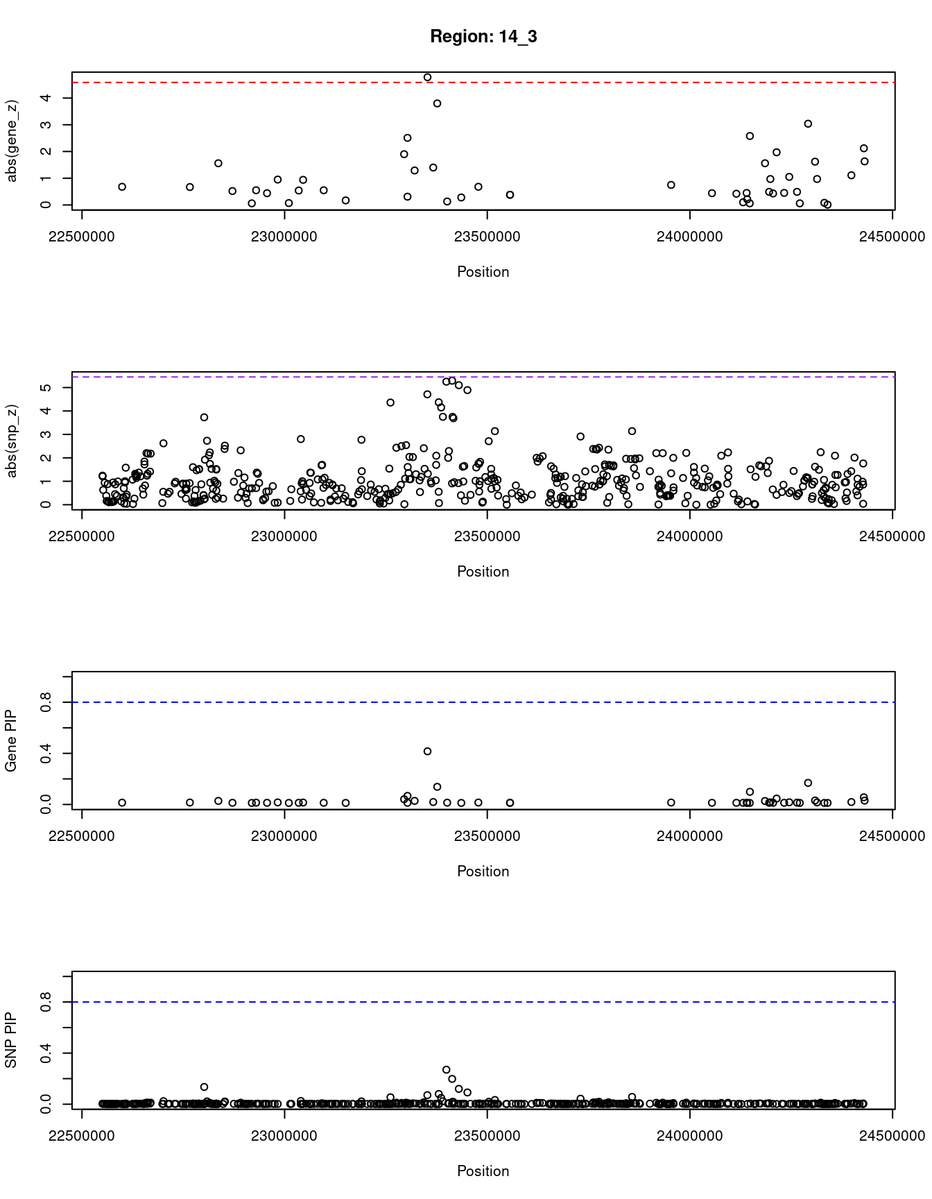
| Version | Author | Date |
|---|---|---|
| 3a7fbc1 | wesleycrouse | 2021-09-08 |
SNPs with highest PIPs
#snps with PIP>0.8 or 20 highest PIPs
head(ctwas_snp_res[order(-ctwas_snp_res$susie_pip),report_cols_snps],
max(sum(ctwas_snp_res$susie_pip>0.8), 20))
id region_tag susie_pip mu2 PVE z
36036 rs72700114 1_83 1.000 59.84 1.8e-04 8.86
102715 rs7568037 2_104 1.000 229.26 6.8e-04 3.74
146915 rs73146926 3_59 1.000 180.40 5.3e-04 3.17
272131 rs280460 5_92 1.000 238.16 7.1e-04 -3.73
673200 rs4257245 17_40 1.000 290.39 8.6e-04 -4.18
36035 rs12142529 1_83 0.999 31.73 9.4e-05 5.85
207639 rs186546224 4_72 0.978 34.36 1.0e-04 -3.71
272126 rs7714176 5_92 0.976 260.25 7.5e-04 3.80
650195 rs60602157 16_39 0.878 26.19 6.8e-05 6.10
207612 rs1906615 4_72 0.821 163.93 4.0e-04 18.79
522447 rs76540106 11_80 0.689 24.34 5.0e-05 -5.07
604044 rs6574343 14_36 0.619 28.15 5.2e-05 4.90
47761 rs80025148 1_109 0.608 28.45 5.1e-05 4.68
207629 rs1906613 4_72 0.585 32.23 5.6e-05 6.06
31838 rs34292822 1_76 0.574 40.02 6.8e-05 7.84
207613 rs75725917 4_72 0.565 150.64 2.5e-04 17.95
650169 rs16971447 16_39 0.546 27.30 4.4e-05 6.53
362075 rs729949 7_70 0.529 29.54 4.6e-05 -7.17
207581 rs1823291 4_72 0.490 80.81 1.2e-04 -11.44
554071 rs6489955 12_69 0.475 25.50 3.6e-05 5.67SNPs with largest effect sizes
#plot PIP vs effect size
plot(ctwas_snp_res$susie_pip, ctwas_snp_res$mu2, xlab="PIP", ylab="mu^2", main="SNP PIPs vs Effect Size")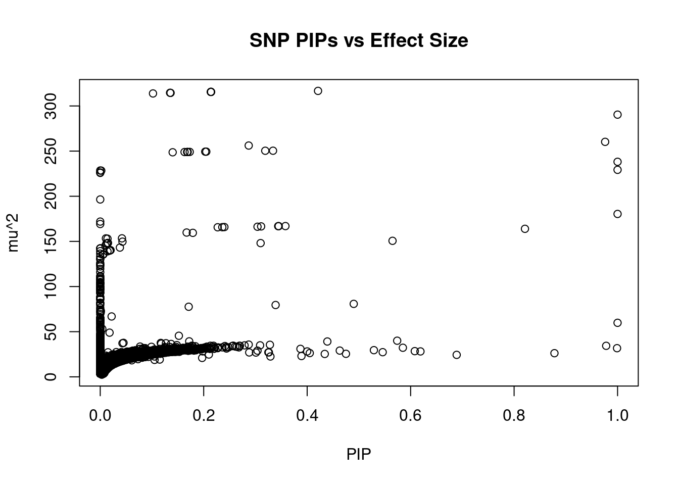
| Version | Author | Date |
|---|---|---|
| 3a7fbc1 | wesleycrouse | 2021-09-08 |
#SNPs with 50 largest effect sizes
head(ctwas_snp_res[order(-ctwas_snp_res$mu2),report_cols_snps],50)
id region_tag susie_pip mu2 PVE z
673208 rs8066344 17_40 0.421 316.68 4.0e-04 4.19
673202 rs7220878 17_40 0.214 315.55 2.0e-04 4.10
673203 rs2366020 17_40 0.214 315.55 2.0e-04 4.10
673204 rs9302905 17_40 0.214 315.55 2.0e-04 4.10
673205 rs9302908 17_40 0.214 315.55 2.0e-04 4.10
673207 rs7224273 17_40 0.214 315.55 2.0e-04 4.10
673199 rs7216073 17_40 0.135 314.57 1.3e-04 4.06
673195 rs9909041 17_40 0.136 314.46 1.3e-04 4.07
673194 rs714769 17_40 0.102 313.84 9.5e-05 4.05
673200 rs4257245 17_40 1.000 290.39 8.6e-04 -4.18
272126 rs7714176 5_92 0.976 260.25 7.5e-04 3.80
272118 rs6883510 5_92 0.287 256.16 2.2e-04 3.71
102712 rs7576894 2_104 0.334 250.42 2.5e-04 -3.74
102716 rs4668385 2_104 0.319 250.39 2.4e-04 -3.77
102726 rs7572334 2_104 0.205 249.40 1.5e-04 -3.74
102731 rs3821084 2_104 0.203 249.39 1.5e-04 -3.74
102728 rs3731981 2_104 0.173 249.10 1.3e-04 -3.72
102729 rs2356781 2_104 0.169 249.05 1.2e-04 -3.72
102725 rs77634005 2_104 0.168 249.04 1.2e-04 -3.71
102733 rs17221367 2_104 0.163 248.98 1.2e-04 -3.71
102721 rs62183502 2_104 0.140 248.69 1.0e-04 -3.69
272131 rs280460 5_92 1.000 238.16 7.1e-04 -3.73
102715 rs7568037 2_104 1.000 229.26 6.8e-04 3.74
272125 rs11739522 5_92 0.000 228.51 3.6e-08 3.58
102717 rs28742013 2_104 0.002 228.37 1.2e-06 -4.15
272137 rs42685 5_92 0.000 226.36 9.4e-09 3.41
272133 rs6860519 5_92 0.000 225.86 5.5e-09 3.32
272134 rs1363743 5_92 0.000 196.45 3.7e-13 3.12
146915 rs73146926 3_59 1.000 180.40 5.3e-04 3.17
102707 rs62183465 2_104 0.000 171.94 1.6e-16 -2.57
272104 rs2431769 5_92 0.000 169.25 6.5e-18 2.46
146916 rs73146943 3_59 0.358 166.96 1.8e-04 -3.15
146917 rs73146950 3_59 0.345 166.88 1.7e-04 -3.15
146918 rs112404167 3_59 0.344 166.87 1.7e-04 -3.14
146920 rs6774870 3_59 0.311 166.59 1.5e-04 -3.13
146922 rs73145304 3_59 0.304 166.23 1.5e-04 -3.14
146921 rs73149115 3_59 0.240 165.88 1.2e-04 -3.09
146914 rs12638777 3_59 0.236 165.74 1.2e-04 -3.09
146913 rs2048521 3_59 0.227 165.64 1.1e-04 -3.08
207612 rs1906615 4_72 0.821 163.93 4.0e-04 18.79
146911 rs12634269 3_59 0.167 159.80 7.9e-05 -3.25
207611 rs2634074 4_72 0.179 159.46 8.5e-05 -18.71
146925 rs819293 3_59 0.042 153.38 1.9e-05 -3.06
146945 rs73153258 3_59 0.011 153.33 5.1e-06 -2.76
146948 rs73153283 3_59 0.014 153.01 6.5e-06 -2.82
207613 rs75725917 4_72 0.565 150.64 2.5e-04 17.95
146899 rs73137393 3_59 0.043 149.70 1.9e-05 -3.25
146908 rs73139131 3_59 0.015 148.27 6.5e-06 -3.05
146906 rs17801380 3_59 0.014 148.21 6.3e-06 -3.03
207610 rs1906611 4_72 0.310 148.11 1.4e-04 17.84SNPs with highest PVE
#SNPs with 50 highest pve
head(ctwas_snp_res[order(-ctwas_snp_res$PVE),report_cols_snps],50)
id region_tag susie_pip mu2 PVE z
673200 rs4257245 17_40 1.000 290.39 8.6e-04 -4.18
272126 rs7714176 5_92 0.976 260.25 7.5e-04 3.80
272131 rs280460 5_92 1.000 238.16 7.1e-04 -3.73
102715 rs7568037 2_104 1.000 229.26 6.8e-04 3.74
146915 rs73146926 3_59 1.000 180.40 5.3e-04 3.17
207612 rs1906615 4_72 0.821 163.93 4.0e-04 18.79
673208 rs8066344 17_40 0.421 316.68 4.0e-04 4.19
102712 rs7576894 2_104 0.334 250.42 2.5e-04 -3.74
207613 rs75725917 4_72 0.565 150.64 2.5e-04 17.95
102716 rs4668385 2_104 0.319 250.39 2.4e-04 -3.77
272118 rs6883510 5_92 0.287 256.16 2.2e-04 3.71
673202 rs7220878 17_40 0.214 315.55 2.0e-04 4.10
673203 rs2366020 17_40 0.214 315.55 2.0e-04 4.10
673204 rs9302905 17_40 0.214 315.55 2.0e-04 4.10
673205 rs9302908 17_40 0.214 315.55 2.0e-04 4.10
673207 rs7224273 17_40 0.214 315.55 2.0e-04 4.10
36036 rs72700114 1_83 1.000 59.84 1.8e-04 8.86
146916 rs73146943 3_59 0.358 166.96 1.8e-04 -3.15
146917 rs73146950 3_59 0.345 166.88 1.7e-04 -3.15
146918 rs112404167 3_59 0.344 166.87 1.7e-04 -3.14
102726 rs7572334 2_104 0.205 249.40 1.5e-04 -3.74
102731 rs3821084 2_104 0.203 249.39 1.5e-04 -3.74
146920 rs6774870 3_59 0.311 166.59 1.5e-04 -3.13
146922 rs73145304 3_59 0.304 166.23 1.5e-04 -3.14
207610 rs1906611 4_72 0.310 148.11 1.4e-04 17.84
102728 rs3731981 2_104 0.173 249.10 1.3e-04 -3.72
673195 rs9909041 17_40 0.136 314.46 1.3e-04 4.07
673199 rs7216073 17_40 0.135 314.57 1.3e-04 4.06
102725 rs77634005 2_104 0.168 249.04 1.2e-04 -3.71
102729 rs2356781 2_104 0.169 249.05 1.2e-04 -3.72
102733 rs17221367 2_104 0.163 248.98 1.2e-04 -3.71
146914 rs12638777 3_59 0.236 165.74 1.2e-04 -3.09
146921 rs73149115 3_59 0.240 165.88 1.2e-04 -3.09
207581 rs1823291 4_72 0.490 80.81 1.2e-04 -11.44
146913 rs2048521 3_59 0.227 165.64 1.1e-04 -3.08
102721 rs62183502 2_104 0.140 248.69 1.0e-04 -3.69
207639 rs186546224 4_72 0.978 34.36 1.0e-04 -3.71
673194 rs714769 17_40 0.102 313.84 9.5e-05 4.05
36035 rs12142529 1_83 0.999 31.73 9.4e-05 5.85
207611 rs2634074 4_72 0.179 159.46 8.5e-05 -18.71
207584 rs2044674 4_72 0.339 79.55 8.0e-05 11.37
146911 rs12634269 3_59 0.167 159.80 7.9e-05 -3.25
31838 rs34292822 1_76 0.574 40.02 6.8e-05 7.84
650195 rs60602157 16_39 0.878 26.19 6.8e-05 6.10
207629 rs1906613 4_72 0.585 32.23 5.6e-05 6.06
604044 rs6574343 14_36 0.619 28.15 5.2e-05 4.90
31837 rs34515871 1_76 0.439 39.14 5.1e-05 7.79
47761 rs80025148 1_109 0.608 28.45 5.1e-05 4.68
522447 rs76540106 11_80 0.689 24.34 5.0e-05 -5.07
362075 rs729949 7_70 0.529 29.54 4.6e-05 -7.17SNPs with largest z scores
#SNPs with 50 largest z scores
head(ctwas_snp_res[order(-abs(ctwas_snp_res$z)),report_cols_snps],50)
id region_tag susie_pip mu2 PVE z
207612 rs1906615 4_72 0.821 163.93 4.0e-04 18.79
207611 rs2634074 4_72 0.179 159.46 8.5e-05 -18.71
207613 rs75725917 4_72 0.565 150.64 2.5e-04 17.95
207610 rs1906611 4_72 0.310 148.11 1.4e-04 17.84
207602 rs4529121 4_72 0.038 143.15 1.6e-05 17.46
207607 rs74496596 4_72 0.020 140.26 8.3e-06 17.43
207606 rs76013973 4_72 0.019 140.11 7.9e-06 17.42
207603 rs12647316 4_72 0.018 139.73 7.3e-06 17.41
207608 rs12639820 4_72 0.014 138.98 6.0e-06 17.39
207609 rs28521134 4_72 0.005 135.34 2.2e-06 17.28
207604 rs12647393 4_72 0.006 135.66 2.3e-06 17.27
207605 rs10019689 4_72 0.006 135.62 2.2e-06 17.27
207596 rs12650829 4_72 0.000 105.03 1.3e-08 14.63
207593 rs60197024 4_72 0.000 99.73 7.3e-09 14.56
207601 rs12644107 4_72 0.000 54.01 8.6e-11 11.66
207617 rs6533530 4_72 0.000 71.87 5.8e-10 -11.49
207581 rs1823291 4_72 0.490 80.81 1.2e-04 -11.44
207587 rs12505886 4_72 0.000 46.15 7.4e-11 -11.39
207618 rs3866831 4_72 0.000 69.41 4.5e-10 -11.38
207584 rs2044674 4_72 0.339 79.55 8.0e-05 11.37
207588 rs112927894 4_72 0.000 44.27 5.2e-11 11.34
207589 rs2723301 4_72 0.000 42.52 4.6e-11 -11.27
207590 rs2595074 4_72 0.000 41.97 4.4e-11 -11.25
207591 rs2723302 4_72 0.000 41.92 4.4e-11 -11.24
207585 rs2723296 4_72 0.171 77.62 3.9e-05 -11.21
207592 rs2218698 4_72 0.000 41.43 4.3e-11 -11.20
207594 rs1584429 4_72 0.000 41.50 4.2e-11 -11.15
207595 rs1448799 4_72 0.000 42.86 4.6e-11 11.14
207597 rs2197814 4_72 0.000 42.92 4.6e-11 11.14
207599 rs2723318 4_72 0.000 41.89 4.3e-11 -11.09
36036 rs72700114 1_83 1.000 59.84 1.8e-04 8.86
207583 rs12642151 4_72 0.000 60.11 1.7e-08 8.76
207576 rs17553596 4_72 0.000 50.67 3.3e-10 7.94
31838 rs34292822 1_76 0.574 40.02 6.8e-05 7.84
31837 rs34515871 1_76 0.439 39.14 5.1e-05 7.79
207637 rs17513625 4_72 0.000 46.41 9.2e-09 7.36
362075 rs729949 7_70 0.529 29.54 4.6e-05 -7.17
362064 rs4727833 7_70 0.124 32.07 1.2e-05 7.15
362076 rs3807990 7_70 0.463 29.08 4.0e-05 -7.14
31840 rs12058931 1_76 0.152 45.49 2.1e-05 7.13
207619 rs4032974 4_72 0.000 37.07 5.2e-11 -6.96
207615 rs4124159 4_72 0.000 36.84 5.1e-11 -6.94
207616 rs10006881 4_72 0.000 36.84 5.1e-11 -6.94
207614 rs1906606 4_72 0.000 36.64 5.0e-11 -6.93
362054 rs1007751 7_70 0.092 28.85 7.9e-06 6.77
362055 rs717957 7_70 0.088 28.62 7.4e-06 6.76
362056 rs28557111 7_70 0.089 28.67 7.5e-06 6.76
362050 rs76160518 7_70 0.113 29.81 1.0e-05 6.74
362046 rs12706089 7_70 0.100 29.28 8.7e-06 6.72
362034 rs2157799 7_70 0.202 32.55 1.9e-05 6.64Gene set enrichment for genes with PIP>0.8
#GO enrichment analysis
library(enrichR)
Welcome to enrichR
Checking connection ... Enrichr ... Connection is Live!
FlyEnrichr ... Connection is available!
WormEnrichr ... Connection is available!
YeastEnrichr ... Connection is available!
FishEnrichr ... Connection is available!dbs <- c("GO_Biological_Process_2021", "GO_Cellular_Component_2021", "GO_Molecular_Function_2021")
genes <- ctwas_gene_res$genename[ctwas_gene_res$susie_pip>0.8]
#number of genes for gene set enrichment
length(genes)[1] 0if (length(genes)>0){
GO_enrichment <- enrichr(genes, dbs)
for (db in dbs){
print(db)
df <- GO_enrichment[[db]]
df <- df[df$Adjusted.P.value<0.05,c("Term", "Overlap", "Adjusted.P.value", "Genes")]
print(df)
}
#DisGeNET enrichment
# devtools::install_bitbucket("ibi_group/disgenet2r")
library(disgenet2r)
disgenet_api_key <- get_disgenet_api_key(
email = "wesleycrouse@gmail.com",
password = "uchicago1" )
Sys.setenv(DISGENET_API_KEY= disgenet_api_key)
res_enrich <-disease_enrichment(entities=genes, vocabulary = "HGNC",
database = "CURATED" )
df <- res_enrich@qresult[1:10, c("Description", "FDR", "Ratio", "BgRatio")]
print(df)
#WebGestalt enrichment
library(WebGestaltR)
background <- ctwas_gene_res$genename
#listGeneSet()
databases <- c("pathway_KEGG", "disease_GLAD4U", "disease_OMIM")
enrichResult <- WebGestaltR(enrichMethod="ORA", organism="hsapiens",
interestGene=genes, referenceGene=background,
enrichDatabase=databases, interestGeneType="genesymbol",
referenceGeneType="genesymbol", isOutput=F)
print(enrichResult[,c("description", "size", "overlap", "FDR", "database", "userId")])
}Sensitivity, specificity and precision for silver standard genes
# library("readxl")
#
# known_annotations <- read_xlsx("data/summary_known_genes_annotations.xlsx", sheet="BMI")
# known_annotations <- unique(known_annotations$`Gene Symbol`)
#
# unrelated_genes <- ctwas_gene_res$genename[!(ctwas_gene_res$genename %in% known_annotations)]
#
# #number of genes in known annotations
# print(length(known_annotations))
#
# #number of genes in known annotations with imputed expression
# print(sum(known_annotations %in% ctwas_gene_res$genename))
#
# #assign ctwas, TWAS, and bystander genes
# ctwas_genes <- ctwas_gene_res$genename[ctwas_gene_res$susie_pip>0.8]
# twas_genes <- ctwas_gene_res$genename[abs(ctwas_gene_res$z)>sig_thresh]
# novel_genes <- ctwas_genes[!(ctwas_genes %in% twas_genes)]
#
# #significance threshold for TWAS
# print(sig_thresh)
#
# #number of ctwas genes
# length(ctwas_genes)
#
# #number of TWAS genes
# length(twas_genes)
#
# #show novel genes (ctwas genes with not in TWAS genes)
# ctwas_gene_res[ctwas_gene_res$genename %in% novel_genes,report_cols]
#
# #sensitivity / recall
# sensitivity <- rep(NA,2)
# names(sensitivity) <- c("ctwas", "TWAS")
# sensitivity["ctwas"] <- sum(ctwas_genes %in% known_annotations)/length(known_annotations)
# sensitivity["TWAS"] <- sum(twas_genes %in% known_annotations)/length(known_annotations)
# sensitivity
#
# #specificity
# specificity <- rep(NA,2)
# names(specificity) <- c("ctwas", "TWAS")
# specificity["ctwas"] <- sum(!(unrelated_genes %in% ctwas_genes))/length(unrelated_genes)
# specificity["TWAS"] <- sum(!(unrelated_genes %in% twas_genes))/length(unrelated_genes)
# specificity
#
# #precision / PPV
# precision <- rep(NA,2)
# names(precision) <- c("ctwas", "TWAS")
# precision["ctwas"] <- sum(ctwas_genes %in% known_annotations)/length(ctwas_genes)
# precision["TWAS"] <- sum(twas_genes %in% known_annotations)/length(twas_genes)
# precision
#
# #ROC curves
#
# pip_range <- (0:1000)/1000
# sensitivity <- rep(NA, length(pip_range))
# specificity <- rep(NA, length(pip_range))
#
# for (index in 1:length(pip_range)){
#   pip <- pip_range[index]
#   ctwas_genes <- ctwas_gene_res$genename[ctwas_gene_res$susie_pip>=pip]
#   sensitivity[index] <- sum(ctwas_genes %in% known_annotations)/length(known_annotations)
#   specificity[index] <- sum(!(unrelated_genes %in% ctwas_genes))/length(unrelated_genes)
# }
#
# plot(1-specificity, sensitivity, type="l", xlim=c(0,1), ylim=c(0,1))
#
# sig_thresh_range <- seq(from=0, to=max(abs(ctwas_gene_res$z)), length.out=length(pip_range))
#
# for (index in 1:length(sig_thresh_range)){
#   sig_thresh_plot <- sig_thresh_range[index]
#   twas_genes <- ctwas_gene_res$genename[abs(ctwas_gene_res$z)>=sig_thresh_plot]
#   sensitivity[index] <- sum(twas_genes %in% known_annotations)/length(known_annotations)
#   specificity[index] <- sum(!(unrelated_genes %in% twas_genes))/length(unrelated_genes)
# }
#
# lines(1-specificity, sensitivity, xlim=c(0,1), ylim=c(0,1), col="red", lty=2)
sessionInfo()R version 3.6.1 (2019-07-05)
Platform: x86_64-pc-linux-gnu (64-bit)
Running under: Scientific Linux 7.4 (Nitrogen)
Matrix products: default
BLAS/LAPACK: /software/openblas-0.2.19-el7-x86_64/lib/libopenblas_haswellp-r0.2.19.so
locale:
[1] LC_CTYPE=en_US.UTF-8 LC_NUMERIC=C
[3] LC_TIME=en_US.UTF-8 LC_COLLATE=en_US.UTF-8
[5] LC_MONETARY=en_US.UTF-8 LC_MESSAGES=en_US.UTF-8
[7] LC_PAPER=en_US.UTF-8 LC_NAME=C
[9] LC_ADDRESS=C LC_TELEPHONE=C
[11] LC_MEASUREMENT=en_US.UTF-8 LC_IDENTIFICATION=C
attached base packages:
[1] stats graphics grDevices utils datasets methods base
other attached packages:
[1] enrichR_3.0 cowplot_1.0.0 ggplot2_3.3.3
loaded via a namespace (and not attached):
[1] tidyselect_1.1.0 xfun_0.8 purrr_0.3.4
[4] colorspace_1.4-1 vctrs_0.3.8 generics_0.0.2
[7] htmltools_0.3.6 yaml_2.2.0 utf8_1.2.1
[10] blob_1.2.1 rlang_0.4.11 later_0.8.0
[13] pillar_1.6.1 glue_1.4.2 withr_2.4.1
[16] DBI_1.1.1 bit64_4.0.5 lifecycle_1.0.0
[19] stringr_1.4.0 munsell_0.5.0 gtable_0.3.0
[22] workflowr_1.6.2 memoise_2.0.0 evaluate_0.14
[25] labeling_0.3 knitr_1.23 fastmap_1.1.0
[28] httpuv_1.5.1 curl_3.3 fansi_0.5.0
[31] Rcpp_1.0.6 promises_1.0.1 scales_1.1.0
[34] cachem_1.0.5 farver_2.1.0 fs_1.3.1
[37] bit_4.0.4 rjson_0.2.20 digest_0.6.20
[40] stringi_1.4.3 dplyr_1.0.7 grid_3.6.1
[43] rprojroot_2.0.2 tools_3.6.1 magrittr_2.0.1
[46] RSQLite_2.2.7 tibble_3.1.2 crayon_1.4.1
[49] whisker_0.3-2 pkgconfig_2.0.3 ellipsis_0.3.2
[52] data.table_1.14.0 rmarkdown_1.13 httr_1.4.1
[55] R6_2.5.0 git2r_0.26.1 compiler_3.6.1