Diagnoses - main ICD10: I48 Atrial fibrillation and flutter - Heart_Atrial_Appendage
wesleycrouse
2021-09-7
Last updated: 2021-09-13
Checks: 7 0
Knit directory: ctwas_applied/
This reproducible R Markdown analysis was created with workflowr (version 1.6.2). The Checks tab describes the reproducibility checks that were applied when the results were created. The Past versions tab lists the development history.
Great! Since the R Markdown file has been committed to the Git repository, you know the exact version of the code that produced these results.
Great job! The global environment was empty. Objects defined in the global environment can affect the analysis in your R Markdown file in unknown ways. For reproduciblity it’s best to always run the code in an empty environment.
The command set.seed(20210726) was run prior to running the code in the R Markdown file. Setting a seed ensures that any results that rely on randomness, e.g. subsampling or permutations, are reproducible.
Great job! Recording the operating system, R version, and package versions is critical for reproducibility.
Nice! There were no cached chunks for this analysis, so you can be confident that you successfully produced the results during this run.
Great job! Using relative paths to the files within your workflowr project makes it easier to run your code on other machines.
Great! You are using Git for version control. Tracking code development and connecting the code version to the results is critical for reproducibility.
The results in this page were generated with repository version 72c8ef7. See the Past versions tab to see a history of the changes made to the R Markdown and HTML files.
Note that you need to be careful to ensure that all relevant files for the analysis have been committed to Git prior to generating the results (you can use wflow_publish or wflow_git_commit). workflowr only checks the R Markdown file, but you know if there are other scripts or data files that it depends on. Below is the status of the Git repository when the results were generated:
working directory clean
Note that any generated files, e.g. HTML, png, CSS, etc., are not included in this status report because it is ok for generated content to have uncommitted changes.
These are the previous versions of the repository in which changes were made to the R Markdown (analysis/ukb-a-536_Heart_Atrial_Appendage_known.Rmd) and HTML (docs/ukb-a-536_Heart_Atrial_Appendage_known.html) files. If you’ve configured a remote Git repository (see ?wflow_git_remote), click on the hyperlinks in the table below to view the files as they were in that past version.
| File | Version | Author | Date | Message |
|---|---|---|---|---|
| html | 7e22565 | wesleycrouse | 2021-09-13 | updating reports |
| html | 3a7fbc1 | wesleycrouse | 2021-09-08 | generating reports for known annotations |
| Rmd | cbf7408 | wesleycrouse | 2021-09-08 | adding enrichment to reports |
Overview
These are the results of a ctwas analysis of the UK Biobank trait Diagnoses - main ICD10: I48 Atrial fibrillation and flutter using Heart_Atrial_Appendage gene weights.
The GWAS was conducted by the Neale Lab, and the biomarker traits we analyzed are discussed here. Summary statistics were obtained from IEU OpenGWAS using GWAS ID: ukb-a-536. Results were obtained from from IEU rather than Neale Lab because they are in a standardard format (GWAS VCF). Note that 3 of the 34 biomarker traits were not available from IEU and were excluded from analysis.
The weights are mashr GTEx v8 models on Heart_Atrial_Appendage eQTL obtained from PredictDB. We performed a full harmonization of the variants, including recovering strand ambiguous variants. This procedure is discussed in a separate document. (TO-DO: add report that describes harmonization)
LD matrices were computed from a 10% subset of Neale lab subjects. Subjects were matched using the plate and well information from genotyping. We included only biallelic variants with MAF>0.01 in the original Neale Lab GWAS. (TO-DO: add more details [number of subjects, variants, etc])
Weight QC
TO-DO: add enhanced QC reporting (total number of weights, why each variant was missing for all genes)
qclist_all <- list()

qc_files <- paste0(results_dir, "/", list.files(results_dir, pattern="exprqc.Rd"))

for (i in 1:length(qc_files)){
  load(qc_files[i])
  chr <- unlist(strsplit(rev(unlist(strsplit(qc_files[i], "_")))[1], "[.]"))[1]
  qclist_all[[chr]] <- cbind(do.call(rbind, lapply(qclist,unlist)), as.numeric(substring(chr,4)))
}

qclist_all <- data.frame(do.call(rbind, qclist_all))
colnames(qclist_all)[ncol(qclist_all)] <- "chr"

rm(qclist, wgtlist, z_gene_chr)

#number of imputed weights
nrow(qclist_all)
[1] 11693#number of imputed weights by chromosome
table(qclist_all$chr)
   1    2    3    4    5    6    7    8    9   10   11   12   13   14   15
1170  827  694  475  535  659  561  417  447  454  708  636  224  401  383
  16   17   18   19   20   21   22
 536  720  185  892  349  128  292
#proportion of imputed weights without missing variants
mean(qclist_all$nmiss==0)[1] 0.7438639Load ctwas results
#load ctwas results
ctwas_res <- data.table::fread(paste0(results_dir, "/", analysis_id, "_ctwas.susieIrss.txt"))

#make unique identifier for regions
ctwas_res$region_tag <- paste(ctwas_res$region_tag1, ctwas_res$region_tag2, sep="_")

#load z scores for SNPs and collect sample size
load(paste0(results_dir, "/", analysis_id, "_expr_z_snp.Rd"))

sample_size <- z_snp$ss
sample_size <- as.numeric(names(which.max(table(sample_size))))

#compute PVE for each gene/SNP
ctwas_res$PVE = ctwas_res$susie_pip*ctwas_res$mu2/sample_size

#separate gene and SNP results
ctwas_gene_res <- ctwas_res[ctwas_res$type == "gene", ]
ctwas_gene_res <- data.frame(ctwas_gene_res)
ctwas_snp_res <- ctwas_res[ctwas_res$type == "SNP", ]
ctwas_snp_res <- data.frame(ctwas_snp_res)

#add gene information to results
sqlite <- RSQLite::dbDriver("SQLite")
db = RSQLite::dbConnect(sqlite, paste0("/project2/compbio/predictdb/mashr_models/mashr_", weight, ".db"))
query <- function(...) RSQLite::dbGetQuery(db, ...)
gene_info <- query("select gene, genename from extra")
gene_info <- query("select gene, genename, gene_type from extra")
RSQLite::dbDisconnect(db)

ctwas_gene_res <- cbind(ctwas_gene_res, gene_info[sapply(ctwas_gene_res$id, match, gene_info$gene), c("genename", "gene_type")])

#add z scores to results
load(paste0(results_dir, "/", analysis_id, "_expr_z_gene.Rd"))
ctwas_gene_res$z <- z_gene[ctwas_gene_res$id,]$z

z_snp <- z_snp[z_snp$id %in% ctwas_snp_res$id,]
ctwas_snp_res$z <- z_snp$z[match(ctwas_snp_res$id, z_snp$id)]

#formatting and rounding for tables
ctwas_gene_res$z <- round(ctwas_gene_res$z,2)
ctwas_snp_res$z <- round(ctwas_snp_res$z,2)
ctwas_gene_res$susie_pip <- round(ctwas_gene_res$susie_pip,3)
ctwas_snp_res$susie_pip <- round(ctwas_snp_res$susie_pip,3)
ctwas_gene_res$mu2 <- round(ctwas_gene_res$mu2,2)
ctwas_snp_res$mu2 <- round(ctwas_snp_res$mu2,2)
ctwas_gene_res$PVE <- signif(ctwas_gene_res$PVE, 2)
ctwas_snp_res$PVE <- signif(ctwas_snp_res$PVE, 2)

#merge gene and snp results with added information
ctwas_snp_res$genename=NA
ctwas_snp_res$gene_type=NA

ctwas_res <- rbind(ctwas_gene_res,
                   ctwas_snp_res[,colnames(ctwas_gene_res)])

#store columns to report
report_cols <- colnames(ctwas_gene_res)[!(colnames(ctwas_gene_res) %in% c("type", "region_tag1", "region_tag2", "cs_index", "gene_type", "z_flag", "id", "chrom", "pos"))]
first_cols <- c("genename", "region_tag")
report_cols <- c(first_cols, report_cols[!(report_cols %in% first_cols)])

report_cols_snps <- c("id", report_cols[-1])

#get number of SNPs from s1 results; adjust for thin
ctwas_res_s1 <- data.table::fread(paste0(results_dir, "/", analysis_id, "_ctwas.s1.susieIrss.txt"))
n_snps <- sum(ctwas_res_s1$type=="SNP")/thin
rm(ctwas_res_s1)
Check convergence of parameters
library(ggplot2)
library(cowplot)
********************************************************Note: As of version 1.0.0, cowplot does not change the default ggplot2 theme anymore. To recover the previous behavior, execute:
theme_set(theme_cowplot())********************************************************load(paste0(results_dir, "/", analysis_id, "_ctwas.s2.susieIrssres.Rd"))
df <- data.frame(niter = rep(1:ncol(group_prior_rec), 2),
value = c(group_prior_rec[1,], group_prior_rec[2,]),
group = rep(c("Gene", "SNP"), each = ncol(group_prior_rec)))
df$group <- as.factor(df$group)
df$value[df$group=="SNP"] <- df$value[df$group=="SNP"]*thin #adjust parameter to account for thin argument
p_pi <- ggplot(df, aes(x=niter, y=value, group=group)) +
geom_line(aes(color=group)) +
geom_point(aes(color=group)) +
xlab("Iteration") + ylab(bquote(pi)) +
ggtitle("Prior mean") +
theme_cowplot()
df <- data.frame(niter = rep(1:ncol(group_prior_var_rec), 2),
value = c(group_prior_var_rec[1,], group_prior_var_rec[2,]),
group = rep(c("Gene", "SNP"), each = ncol(group_prior_var_rec)))
df$group <- as.factor(df$group)
p_sigma2 <- ggplot(df, aes(x=niter, y=value, group=group)) +
geom_line(aes(color=group)) +
geom_point(aes(color=group)) +
xlab("Iteration") + ylab(bquote(sigma^2)) +
ggtitle("Prior variance") +
theme_cowplot()
plot_grid(p_pi, p_sigma2)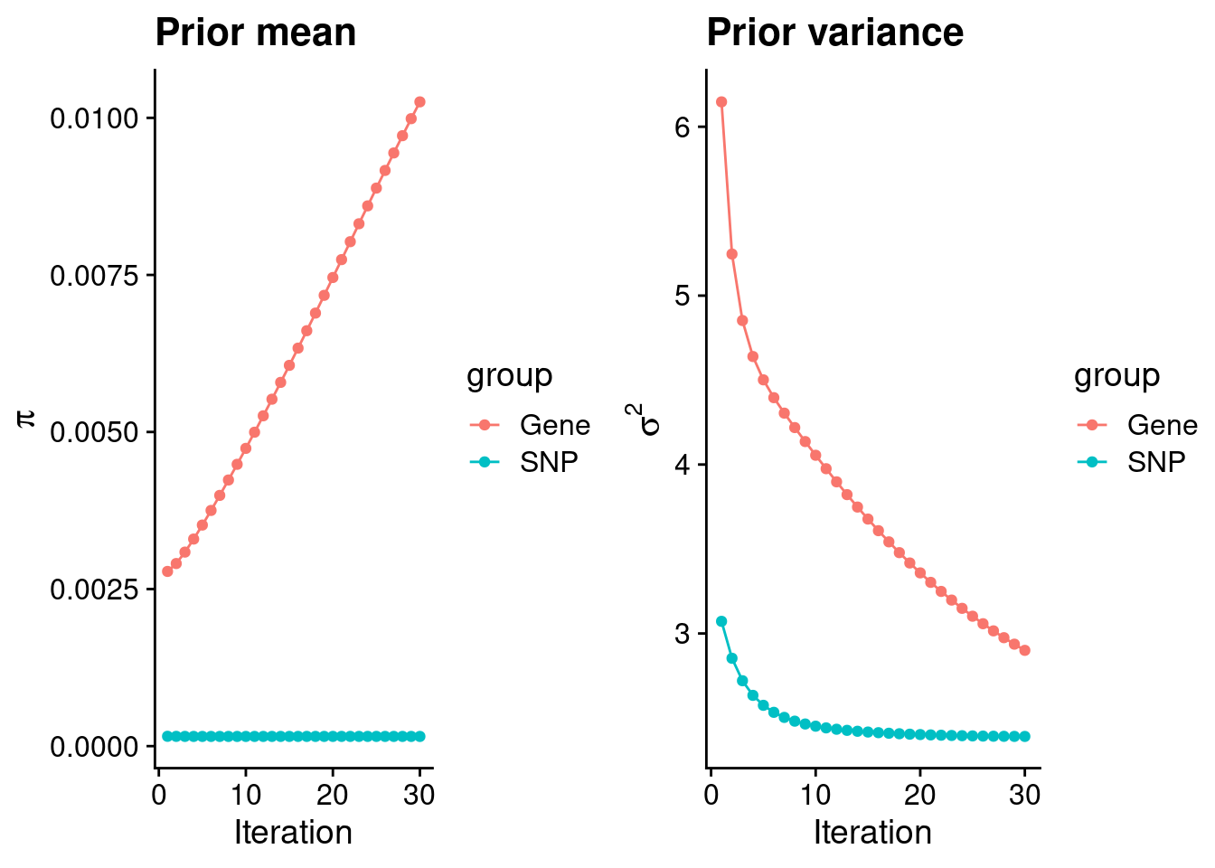
| Version | Author | Date |
|---|---|---|
| 3a7fbc1 | wesleycrouse | 2021-09-08 |
#estimated group prior
estimated_group_prior <- group_prior_rec[,ncol(group_prior_rec)]
names(estimated_group_prior) <- c("gene", "snp")
estimated_group_prior["snp"] <- estimated_group_prior["snp"]*thin #adjust parameter to account for thin argument
print(estimated_group_prior)
gene snp
0.0102546783 0.0001540992 #estimated group prior variance
estimated_group_prior_var <- group_prior_var_rec[,ncol(group_prior_var_rec)]
names(estimated_group_prior_var) <- c("gene", "snp")
print(estimated_group_prior_var) gene snp
2.899979 2.390344 #report sample size
print(sample_size)[1] 337199#report group size
group_size <- c(nrow(ctwas_gene_res), n_snps)
print(group_size)[1] 11693 7535010#estimated group PVE
estimated_group_pve <- estimated_group_prior_var*estimated_group_prior*group_size/sample_size #check PVE calculation
names(estimated_group_pve) <- c("gene", "snp")
print(estimated_group_pve) gene snp
0.001031232 0.008231110 #compare sum(PIP*mu2/sample_size) with above PVE calculation
c(sum(ctwas_gene_res$PVE),sum(ctwas_snp_res$PVE))[1] 0.0121411 0.1342480Genes with highest PIPs
#distribution of PIPs
hist(ctwas_gene_res$susie_pip, xlim=c(0,1), main="Distribution of Gene PIPs")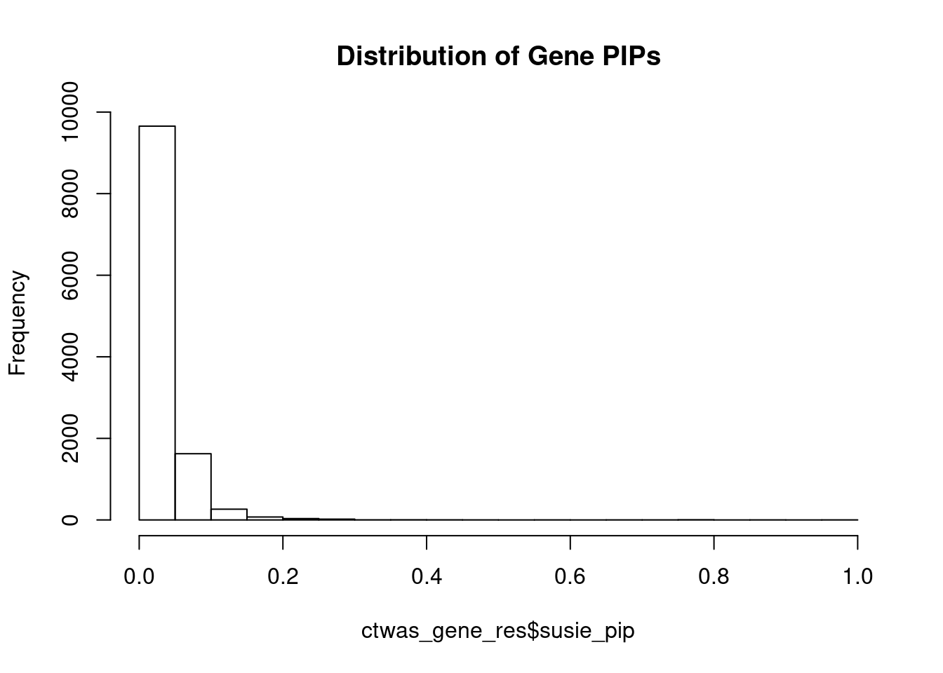
| Version | Author | Date |
|---|---|---|
| 3a7fbc1 | wesleycrouse | 2021-09-08 |
#genes with PIP>0.8 or 20 highest PIPs
head(ctwas_gene_res[order(-ctwas_gene_res$susie_pip),report_cols], max(sum(ctwas_gene_res$susie_pip>0.8), 20))
genename region_tag susie_pip mu2 PVE z
6621 AKAP6 14_8 0.955 21.93 6.2e-05 -5.07
1411 SLC22A17 14_3 0.884 20.88 5.5e-05 -4.77
3250 WIPF1 2_105 0.797 21.88 5.2e-05 4.90
3275 PRRX1 1_84 0.789 26.30 6.2e-05 5.54
12836 RP11-325L7.2 5_82 0.789 21.48 5.0e-05 5.07
2292 CAV2 7_70 0.785 37.18 8.7e-05 7.39
541 PKP2 12_22 0.755 19.74 4.4e-05 4.48
13617 POM121C 7_48 0.734 20.23 4.4e-05 -4.24
10898 NCCRP1 19_26 0.686 23.56 4.8e-05 -4.37
3858 SSPN 12_18 0.664 23.13 4.6e-05 -5.20
2465 PITX3 10_65 0.590 22.88 4.0e-05 -5.34
4009 DEK 6_14 0.568 22.46 3.8e-05 -5.25
8247 IL25 14_3 0.461 21.03 2.9e-05 -4.29
8101 KDM1B 6_14 0.435 21.78 2.8e-05 -5.14
3665 KCNJ5 11_80 0.428 27.54 3.5e-05 -4.19
6869 FAM134B 5_12 0.422 25.90 3.2e-05 3.73
3088 GNB4 3_110 0.393 25.30 2.9e-05 -3.68
13075 LINC01629 14_36 0.374 22.33 2.5e-05 -4.17
12415 AC004947.2 7_23 0.359 24.77 2.6e-05 3.84
8260 FBN1 15_19 0.352 24.15 2.5e-05 3.44Genes with largest effect sizes
#plot PIP vs effect size
plot(ctwas_gene_res$susie_pip, ctwas_gene_res$mu2, xlab="PIP", ylab="mu^2", main="Gene PIPs vs Effect Size")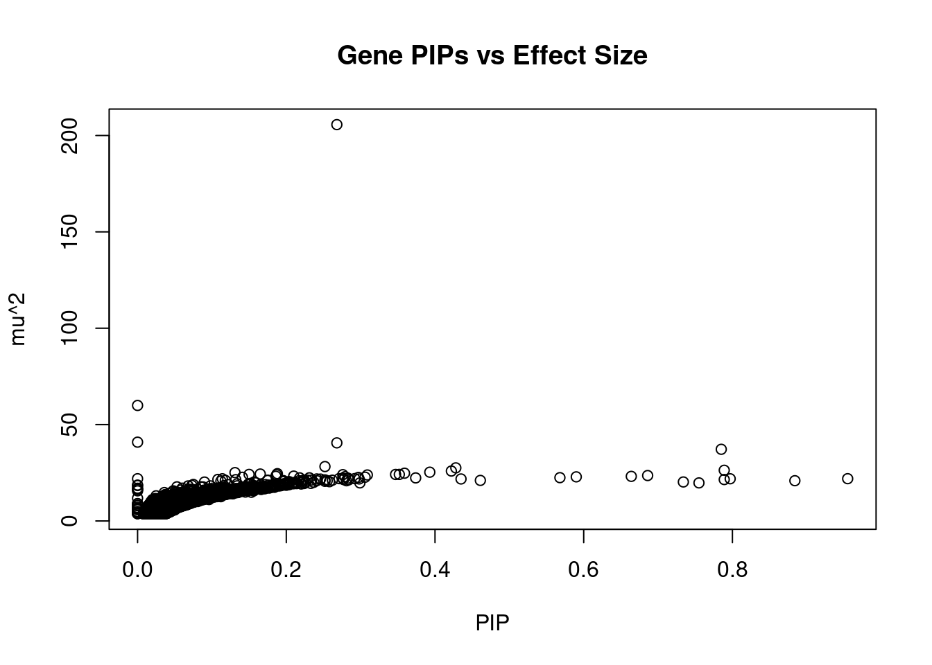
| Version | Author | Date |
|---|---|---|
| 3a7fbc1 | wesleycrouse | 2021-09-08 |
#genes with 20 largest effect sizes
head(ctwas_gene_res[order(-ctwas_gene_res$mu2),report_cols],20)
genename region_tag susie_pip mu2 PVE z
3894 METTL8 2_104 0.268 205.65 1.6e-04 -3.72
9893 STX19 3_59 0.000 59.93 1.9e-13 0.17
9886 NSUN3 3_59 0.000 40.88 4.6e-13 -1.48
2293 CAV1 7_70 0.268 40.51 3.2e-05 7.16
2292 CAV2 7_70 0.785 37.18 8.7e-05 7.39
7059 FBXO32 8_80 0.252 28.22 2.1e-05 -4.07
3665 KCNJ5 11_80 0.428 27.54 3.5e-05 -4.19
3275 PRRX1 1_84 0.789 26.30 6.2e-05 5.54
6869 FAM134B 5_12 0.422 25.90 3.2e-05 3.73
3088 GNB4 3_110 0.393 25.30 2.9e-05 -3.68
2476 SH3PXD2A 10_66 0.131 25.08 9.8e-06 4.00
12415 AC004947.2 7_23 0.359 24.77 2.6e-05 3.84
1316 TBX5 12_69 0.188 24.53 1.4e-05 -4.17
11174 AP2A1 19_35 0.165 24.34 1.2e-05 3.23
12013 ZSWIM8 10_49 0.150 24.15 1.1e-05 -3.21
8260 FBN1 15_19 0.352 24.15 2.5e-05 3.44
7860 LIPH 3_114 0.347 24.13 2.5e-05 3.84
6847 NUS1 6_78 0.276 24.01 2.0e-05 3.39
7111 DHRS1 14_3 0.187 23.97 1.3e-05 3.07
4671 EIF5A 17_6 0.309 23.86 2.2e-05 -3.65Genes with highest PVE
#genes with 20 highest pve
head(ctwas_gene_res[order(-ctwas_gene_res$PVE),report_cols],20)
genename region_tag susie_pip mu2 PVE z
3894 METTL8 2_104 0.268 205.65 1.6e-04 -3.72
2292 CAV2 7_70 0.785 37.18 8.7e-05 7.39
3275 PRRX1 1_84 0.789 26.30 6.2e-05 5.54
6621 AKAP6 14_8 0.955 21.93 6.2e-05 -5.07
1411 SLC22A17 14_3 0.884 20.88 5.5e-05 -4.77
3250 WIPF1 2_105 0.797 21.88 5.2e-05 4.90
12836 RP11-325L7.2 5_82 0.789 21.48 5.0e-05 5.07
10898 NCCRP1 19_26 0.686 23.56 4.8e-05 -4.37
3858 SSPN 12_18 0.664 23.13 4.6e-05 -5.20
13617 POM121C 7_48 0.734 20.23 4.4e-05 -4.24
541 PKP2 12_22 0.755 19.74 4.4e-05 4.48
2465 PITX3 10_65 0.590 22.88 4.0e-05 -5.34
4009 DEK 6_14 0.568 22.46 3.8e-05 -5.25
3665 KCNJ5 11_80 0.428 27.54 3.5e-05 -4.19
6869 FAM134B 5_12 0.422 25.90 3.2e-05 3.73
2293 CAV1 7_70 0.268 40.51 3.2e-05 7.16
3088 GNB4 3_110 0.393 25.30 2.9e-05 -3.68
8247 IL25 14_3 0.461 21.03 2.9e-05 -4.29
8101 KDM1B 6_14 0.435 21.78 2.8e-05 -5.14
12415 AC004947.2 7_23 0.359 24.77 2.6e-05 3.84Genes with largest z scores
#genes with 20 largest z scores
head(ctwas_gene_res[order(-abs(ctwas_gene_res$z)),report_cols],20)
genename region_tag susie_pip mu2 PVE z
2292 CAV2 7_70 0.785 37.18 8.7e-05 7.39
2293 CAV1 7_70 0.268 40.51 3.2e-05 7.16
3275 PRRX1 1_84 0.789 26.30 6.2e-05 5.54
2465 PITX3 10_65 0.590 22.88 4.0e-05 -5.34
4009 DEK 6_14 0.568 22.46 3.8e-05 -5.25
3858 SSPN 12_18 0.664 23.13 4.6e-05 -5.20
8101 KDM1B 6_14 0.435 21.78 2.8e-05 -5.14
12836 RP11-325L7.2 5_82 0.789 21.48 5.0e-05 5.07
6621 AKAP6 14_8 0.955 21.93 6.2e-05 -5.07
3250 WIPF1 2_105 0.797 21.88 5.2e-05 4.90
7730 PBXIP1 1_76 0.141 22.66 9.5e-06 -4.81
1411 SLC22A17 14_3 0.884 20.88 5.5e-05 -4.77
7733 DCST2 1_76 0.114 21.88 7.4e-06 -4.59
541 PKP2 12_22 0.755 19.74 4.4e-05 4.48
10898 NCCRP1 19_26 0.686 23.56 4.8e-05 -4.37
8247 IL25 14_3 0.461 21.03 2.9e-05 -4.29
13617 POM121C 7_48 0.734 20.23 4.4e-05 -4.24
13511 RP11-346C20.3 16_39 0.039 13.28 1.5e-06 4.22
5288 TPMT 6_14 0.186 23.18 1.3e-05 -4.19
3665 KCNJ5 11_80 0.428 27.54 3.5e-05 -4.19Comparing z scores and PIPs
#set nominal signifiance threshold for z scores
alpha <- 0.05

#bonferroni adjusted threshold for z scores
sig_thresh <- qnorm(1-(alpha/nrow(ctwas_gene_res)/2), lower=T)

#Q-Q plot for z scores
obs_z <- ctwas_gene_res$z[order(ctwas_gene_res$z)]
exp_z <- qnorm((1:nrow(ctwas_gene_res))/nrow(ctwas_gene_res))

plot(exp_z, obs_z, xlab="Expected z", ylab="Observed z", main="Gene z score Q-Q plot")
abline(a=0,b=1)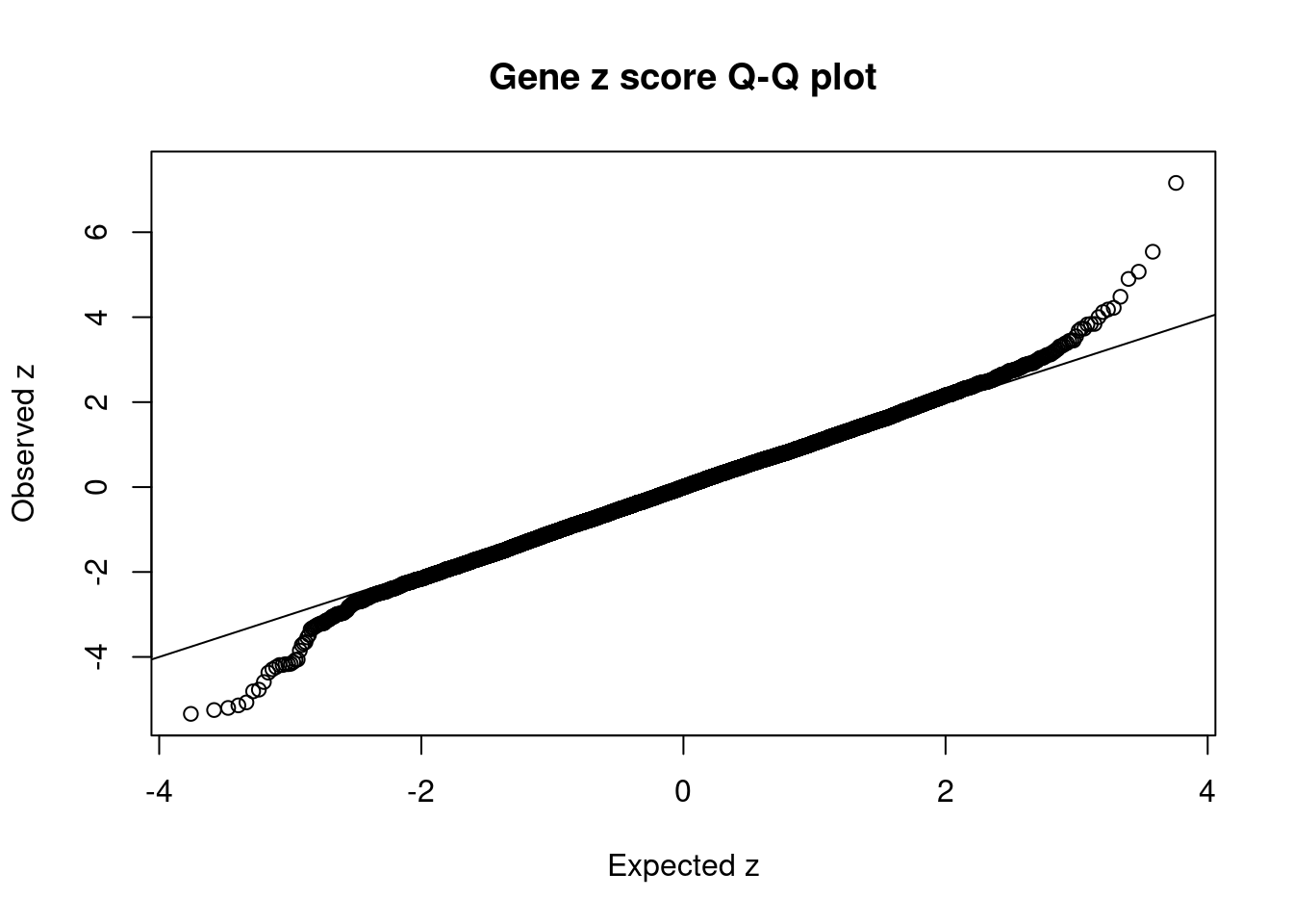
| Version | Author | Date |
|---|---|---|
| 3a7fbc1 | wesleycrouse | 2021-09-08 |
#plot z score vs PIP
plot(abs(ctwas_gene_res$z), ctwas_gene_res$susie_pip, xlab="abs(z)", ylab="PIP")
abline(v=sig_thresh, col="red", lty=2)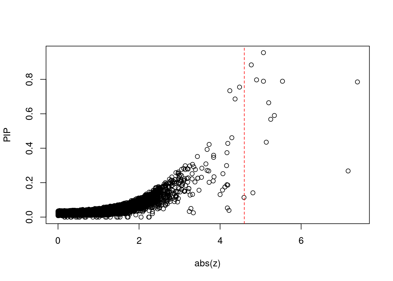
| Version | Author | Date |
|---|---|---|
| 3a7fbc1 | wesleycrouse | 2021-09-08 |
#proportion of significant z scores
mean(abs(ctwas_gene_res$z) > sig_thresh)
[1] 0.001026255#genes with most significant z scores
head(ctwas_gene_res[order(-abs(ctwas_gene_res$z)),report_cols],20) genename region_tag susie_pip mu2 PVE z
2292 CAV2 7_70 0.785 37.18 8.7e-05 7.39
2293 CAV1 7_70 0.268 40.51 3.2e-05 7.16
3275 PRRX1 1_84 0.789 26.30 6.2e-05 5.54
2465 PITX3 10_65 0.590 22.88 4.0e-05 -5.34
4009 DEK 6_14 0.568 22.46 3.8e-05 -5.25
3858 SSPN 12_18 0.664 23.13 4.6e-05 -5.20
8101 KDM1B 6_14 0.435 21.78 2.8e-05 -5.14
12836 RP11-325L7.2 5_82 0.789 21.48 5.0e-05 5.07
6621 AKAP6 14_8 0.955 21.93 6.2e-05 -5.07
3250 WIPF1 2_105 0.797 21.88 5.2e-05 4.90
7730 PBXIP1 1_76 0.141 22.66 9.5e-06 -4.81
1411 SLC22A17 14_3 0.884 20.88 5.5e-05 -4.77
7733 DCST2 1_76 0.114 21.88 7.4e-06 -4.59
541 PKP2 12_22 0.755 19.74 4.4e-05 4.48
10898 NCCRP1 19_26 0.686 23.56 4.8e-05 -4.37
8247 IL25 14_3 0.461 21.03 2.9e-05 -4.29
13617 POM121C 7_48 0.734 20.23 4.4e-05 -4.24
13511 RP11-346C20.3 16_39 0.039 13.28 1.5e-06 4.22
5288 TPMT 6_14 0.186 23.18 1.3e-05 -4.19
3665 KCNJ5 11_80 0.428 27.54 3.5e-05 -4.19Locus plots for genes and SNPs
ctwas_gene_res_sortz <- ctwas_gene_res[order(-abs(ctwas_gene_res$z)),]

n_plots <- 5
for (region_tag_plot in head(unique(ctwas_gene_res_sortz$region_tag), n_plots)){
  ctwas_res_region <-  ctwas_res[ctwas_res$region_tag==region_tag_plot,]
  start <- min(ctwas_res_region$pos)
  end <- max(ctwas_res_region$pos)

  ctwas_res_region <- ctwas_res_region[order(ctwas_res_region$pos),]
  ctwas_res_region_gene <- ctwas_res_region[ctwas_res_region$type=="gene",]
  ctwas_res_region_snp <- ctwas_res_region[ctwas_res_region$type=="SNP",]

  #region name
  print(paste0("Region: ", region_tag_plot))

  #table of genes in region
  print(ctwas_res_region_gene[,report_cols])

  par(mfrow=c(4,1))

  #gene z scores
  plot(ctwas_res_region_gene$pos, abs(ctwas_res_region_gene$z), xlab="Position", ylab="abs(gene_z)", xlim=c(start,end),
   ylim=c(0,max(sig_thresh, abs(ctwas_res_region_gene$z))),
   main=paste0("Region: ", region_tag_plot))
  abline(h=sig_thresh,col="red",lty=2)

  #significance threshold for SNPs
  alpha_snp <- 5*10^(-8)
  sig_thresh_snp <- qnorm(1-alpha_snp/2, lower=T)

  #snp z scores
  plot(ctwas_res_region_snp$pos, abs(ctwas_res_region_snp$z), xlab="Position", ylab="abs(snp_z)",xlim=c(start,end),
   ylim=c(0,max(sig_thresh_snp, max(abs(ctwas_res_region_snp$z)))))
  abline(h=sig_thresh_snp,col="purple",lty=2)

  #gene pips
  plot(ctwas_res_region_gene$pos, ctwas_res_region_gene$susie_pip, xlab="Position", ylab="Gene PIP", xlim=c(start,end), ylim=c(0,1))
  abline(h=0.8,col="blue",lty=2)

  #snp pips
  plot(ctwas_res_region_snp$pos, ctwas_res_region_snp$susie_pip, xlab="Position", ylab="SNP PIP", xlim=c(start,end), ylim=c(0,1))
  abline(h=0.8,col="blue",lty=2)
}
[1] "Region: 7_70"
genename region_tag susie_pip mu2 PVE z
9316 LRRN3 7_70 0.011 5.79 1.9e-07 0.88
10486 IMMP2L 7_70 0.013 6.89 2.6e-07 -1.10
10096 LSMEM1 7_70 0.020 10.32 6.1e-07 1.58
6325 TMEM168 7_70 0.009 4.07 1.0e-07 -0.38
8015 GPR85 7_70 0.014 7.88 3.4e-07 1.24
8014 BMT2 7_70 0.023 11.47 7.9e-07 1.75
12439 HRAT17 7_70 0.010 5.02 1.5e-07 0.69
11985 LINC00998 7_70 0.011 5.86 1.9e-07 -0.91
6892 PPP1R3A 7_70 0.014 7.49 3.0e-07 -1.20
4991 MDFIC 7_70 0.010 4.93 1.4e-07 -0.54
4990 TES 7_70 0.008 3.77 9.3e-08 -0.09
2292 CAV2 7_70 0.785 37.18 8.7e-05 7.39
2293 CAV1 7_70 0.268 40.51 3.2e-05 7.16
11541 CAPZA2 7_70 0.018 10.04 5.5e-07 -1.77
| Version | Author | Date |
|---|---|---|
| 3a7fbc1 | wesleycrouse | 2021-09-08 |
[1] "Region: 1_84"
        genename region_tag susie_pip   mu2     PVE     z
3275       PRRX1       1_84     0.789 26.30 6.2e-05  5.54
13556 RP1-79C4.4       1_84     0.025 13.04 9.7e-07  3.34
132         FMO3       1_84     0.019  4.62 2.6e-07  0.67
1450        FMO2       1_84     0.017  3.79 1.9e-07  0.14
964         FMO4       1_84     0.017  3.80 1.9e-07  0.27
364         MYOC       1_84     0.019  4.42 2.4e-07 -0.53
3427       VAMP4       1_84     0.018  4.17 2.2e-07 -0.45
11344       DNM3       1_84     0.018  4.10 2.2e-07 -0.37
5075        PIGC       1_84     0.017  3.73 1.9e-07 -0.09
10093   C1orf105       1_84     0.017  3.85 2.0e-07  0.20
1451        SUCO       1_84     0.020  4.86 2.8e-07 -0.71
3428       FASLG       1_84     0.017  3.73 1.9e-07  0.06
| Version | Author | Date |
|---|---|---|
| 3a7fbc1 | wesleycrouse | 2021-09-08 |
[1] "Region: 10_65"
      genename region_tag susie_pip   mu2     PVE     z
8266      POLL      10_65     0.031  6.51 6.0e-07  1.38
8268      DPCD      10_65     0.023  3.95 2.7e-07 -0.25
2463      NPM3      10_65     0.031  8.46 7.8e-07  2.33
11418    MGEA5      10_65     0.023  4.15 2.8e-07 -0.72
3633    KCNIP2      10_65     0.023  3.89 2.7e-07  0.25
3632  C10orf76      10_65     0.032  7.36 6.9e-07  1.88
8273      HPS6      10_65     0.029  6.98 6.1e-07 -1.77
11482     LDB1      10_65     0.028  6.03 4.9e-07  1.57
6462     PPRC1      10_65     0.024  4.46 3.2e-07  0.79
8275     NOLC1      10_65     0.023  3.87 2.6e-07  0.47
3618    ELOVL3      10_65     0.024  4.91 3.5e-07  1.39
2465     PITX3      10_65     0.590 22.88 4.0e-05 -5.34
569        PSD      10_65     0.035  7.33 7.5e-07  1.42
5402   MFSD13A      10_65     0.024  4.19 3.0e-07  0.50
2468      SUFU      10_65     0.028  5.49 4.6e-07  0.96
| Version | Author | Date |
|---|---|---|
| 3a7fbc1 | wesleycrouse | 2021-09-08 |
[1] "Region: 6_14"
      genename region_tag susie_pip   mu2     PVE     z
5295    FAM8A1       6_14     0.031  5.22 4.7e-07 -0.64
4008    NUP153       6_14     0.032  5.58 5.4e-07  0.68
5261    KIF13A       6_14     0.025  3.90 2.9e-07 -0.36
5288      TPMT       6_14     0.186 23.18 1.3e-05 -4.19
10795   NHLRC1       6_14     0.028  4.43 3.6e-07  0.21
8101     KDM1B       6_14     0.435 21.78 2.8e-05 -5.14
4009       DEK       6_14     0.568 22.46 3.8e-05 -5.25
5290   RNF144B       6_14     0.033  9.49 9.1e-07 -3.24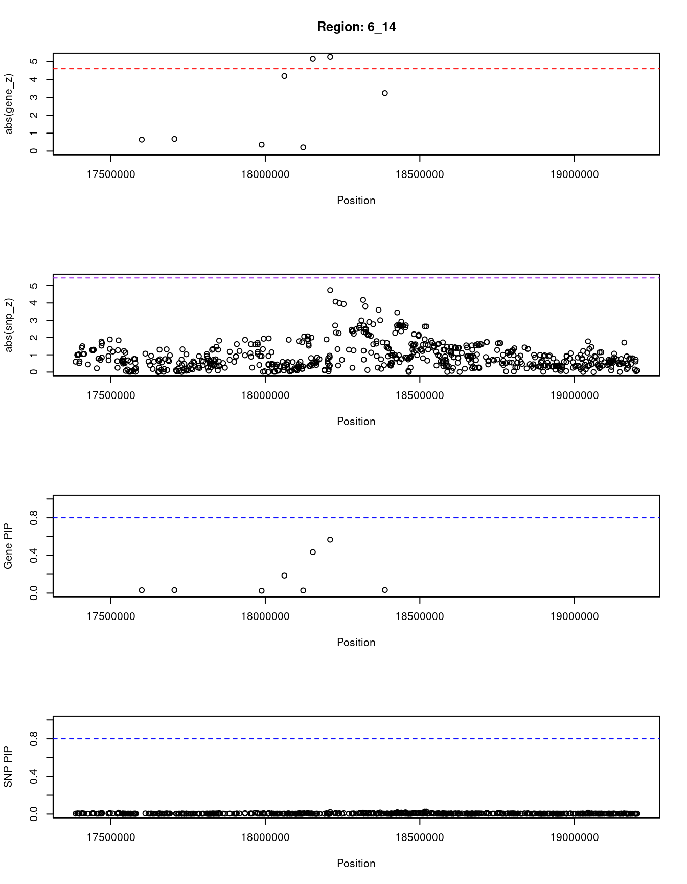
| Version | Author | Date |
|---|---|---|
| 3a7fbc1 | wesleycrouse | 2021-09-08 |
[1] "Region: 12_18"
           genename region_tag susie_pip   mu2     PVE     z
13966 RP11-707G18.1      12_18     0.033 10.21 9.9e-07 -1.68
3857         RASSF8      12_18     0.098 18.20 5.3e-06 -2.57
3858           SSPN      12_18     0.664 23.13 4.6e-05 -5.20
3859          ITPR2      12_18     0.015  4.19 1.8e-07 -0.48
616          INTS13      12_18     0.029  9.35 8.0e-07 -1.53
2842       FGFR1OP2      12_18     0.029  9.35 8.0e-07  1.53
617          TM7SF3      12_18     0.015  4.33 1.9e-07 -0.66
13846  RP11-582E3.6      12_18     0.018  5.86 3.1e-07  1.06
6771          MED21      12_18     0.037 11.33 1.2e-06 -1.87
12016      C12orf71      12_18     0.015  4.27 1.9e-07  0.49
11861        STK38L      12_18     0.014  3.72 1.5e-07 -0.09
332          ARNTL2      12_18     0.070 15.77 3.3e-06 -2.11
8224          SMCO2      12_18     0.017  5.43 2.8e-07 -0.88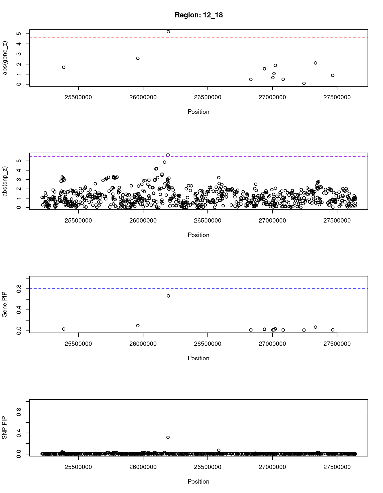
| Version | Author | Date |
|---|---|---|
| 3a7fbc1 | wesleycrouse | 2021-09-08 |
SNPs with highest PIPs
#snps with PIP>0.8 or 20 highest PIPs
head(ctwas_snp_res[order(-ctwas_snp_res$susie_pip),report_cols_snps],
max(sum(ctwas_snp_res$susie_pip>0.8), 20))
id region_tag susie_pip mu2 PVE z
36036 rs72700114 1_83 1.000 59.33 1.8e-04 8.86
102715 rs7568037 2_104 1.000 225.51 6.7e-04 3.74
146915 rs73146926 3_59 1.000 165.69 4.9e-04 3.17
271623 rs280460 5_92 1.000 217.91 6.5e-04 -3.73
671407 rs4257245 17_40 1.000 265.86 7.9e-04 -4.18
36035 rs12142529 1_83 0.999 31.32 9.3e-05 5.85
207639 rs186546224 4_72 0.976 33.73 9.8e-05 -3.71
271618 rs7714176 5_92 0.972 239.51 6.9e-04 3.80
648402 rs60602157 16_39 0.853 26.56 6.7e-05 6.10
207612 rs1906615 4_72 0.818 162.85 3.9e-04 18.79
521939 rs76540106 11_80 0.664 24.69 4.9e-05 -5.07
207629 rs1906613 4_72 0.584 31.91 5.5e-05 6.06
47761 rs80025148 1_109 0.574 29.28 5.0e-05 4.68
31838 rs34292822 1_76 0.573 39.36 6.7e-05 7.84
207613 rs75725917 4_72 0.563 149.49 2.5e-04 17.95
648376 rs16971447 16_39 0.544 27.21 4.4e-05 6.53
207581 rs1823291 4_72 0.489 80.24 1.2e-04 -11.44
553563 rs6489955 12_69 0.457 25.32 3.4e-05 5.67
31837 rs34515871 1_76 0.441 38.48 5.0e-05 7.79
602251 rs6574343 14_36 0.424 30.16 3.8e-05 4.90SNPs with largest effect sizes
#plot PIP vs effect size
plot(ctwas_snp_res$susie_pip, ctwas_snp_res$mu2, xlab="PIP", ylab="mu^2", main="SNP PIPs vs Effect Size")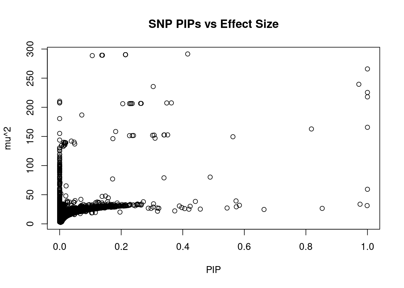
| Version | Author | Date |
|---|---|---|
| 3a7fbc1 | wesleycrouse | 2021-09-08 |
#SNPs with 50 largest effect sizes
head(ctwas_snp_res[order(-ctwas_snp_res$mu2),report_cols_snps],50)
id region_tag susie_pip mu2 PVE z
671415 rs8066344 17_40 0.416 291.52 3.6e-04 4.19
671409 rs7220878 17_40 0.214 290.34 1.8e-04 4.10
671410 rs2366020 17_40 0.214 290.34 1.8e-04 4.10
671411 rs9302905 17_40 0.214 290.34 1.8e-04 4.10
671412 rs9302908 17_40 0.214 290.34 1.8e-04 4.10
671414 rs7224273 17_40 0.214 290.34 1.8e-04 4.10
671406 rs7216073 17_40 0.137 289.39 1.2e-04 4.06
671402 rs9909041 17_40 0.139 289.31 1.2e-04 4.07
671401 rs714769 17_40 0.106 288.71 9.1e-05 4.05
671407 rs4257245 17_40 1.000 265.86 7.9e-04 -4.18
271618 rs7714176 5_92 0.972 239.51 6.9e-04 3.80
271610 rs6883510 5_92 0.304 235.63 2.1e-04 3.71
102715 rs7568037 2_104 1.000 225.51 6.7e-04 3.74
271623 rs280460 5_92 1.000 217.91 6.5e-04 -3.73
271617 rs11739522 5_92 0.000 210.37 6.3e-08 3.58
271629 rs42685 5_92 0.000 208.18 1.7e-08 3.41
271625 rs6860519 5_92 0.000 207.60 1.0e-08 3.32
102712 rs7576894 2_104 0.363 207.56 2.2e-04 -3.74
102716 rs4668385 2_104 0.348 207.45 2.1e-04 -3.77
102731 rs3821084 2_104 0.263 206.67 1.6e-04 -3.74
102726 rs7572334 2_104 0.265 206.65 1.6e-04 -3.74
102728 rs3731981 2_104 0.236 206.47 1.4e-04 -3.72
102729 rs2356781 2_104 0.232 206.43 1.4e-04 -3.72
102725 rs77634005 2_104 0.231 206.42 1.4e-04 -3.71
102733 rs17221367 2_104 0.227 206.38 1.4e-04 -3.71
102721 rs62183502 2_104 0.205 206.18 1.3e-04 -3.69
102717 rs28742013 2_104 0.072 186.80 4.0e-05 -4.15
271626 rs1363743 5_92 0.000 180.64 1.3e-12 3.12
146915 rs73146926 3_59 1.000 165.69 4.9e-04 3.17
207612 rs1906615 4_72 0.818 162.85 3.9e-04 18.79
207611 rs2634074 4_72 0.182 158.46 8.6e-05 -18.71
271596 rs2431769 5_92 0.000 155.16 4.0e-17 2.46
146916 rs73146943 3_59 0.351 152.66 1.6e-04 -3.15
146917 rs73146950 3_59 0.340 152.57 1.5e-04 -3.15
146918 rs112404167 3_59 0.339 152.56 1.5e-04 -3.14
146920 rs6774870 3_59 0.307 152.30 1.4e-04 -3.13
146922 rs73145304 3_59 0.302 151.98 1.4e-04 -3.14
146921 rs73149115 3_59 0.240 151.61 1.1e-04 -3.09
146914 rs12638777 3_59 0.236 151.48 1.1e-04 -3.09
146913 rs2048521 3_59 0.227 151.39 1.0e-04 -3.08
207613 rs75725917 4_72 0.563 149.49 2.5e-04 17.95
207610 rs1906611 4_72 0.310 146.98 1.4e-04 17.84
146911 rs12634269 3_59 0.173 146.22 7.5e-05 -3.25
102707 rs62183465 2_104 0.000 143.77 2.7e-10 -2.57
207602 rs4529121 4_72 0.038 142.06 1.6e-05 17.46
146925 rs819293 3_59 0.047 140.28 2.0e-05 -3.06
146945 rs73153258 3_59 0.013 139.94 5.4e-06 -2.76
146948 rs73153283 3_59 0.017 139.72 6.9e-06 -2.82
207607 rs74496596 4_72 0.020 139.20 8.4e-06 17.43
207606 rs76013973 4_72 0.019 139.06 8.0e-06 17.42SNPs with highest PVE
#SNPs with 50 highest pve
head(ctwas_snp_res[order(-ctwas_snp_res$PVE),report_cols_snps],50)
id region_tag susie_pip mu2 PVE z
671407 rs4257245 17_40 1.000 265.86 7.9e-04 -4.18
271618 rs7714176 5_92 0.972 239.51 6.9e-04 3.80
102715 rs7568037 2_104 1.000 225.51 6.7e-04 3.74
271623 rs280460 5_92 1.000 217.91 6.5e-04 -3.73
146915 rs73146926 3_59 1.000 165.69 4.9e-04 3.17
207612 rs1906615 4_72 0.818 162.85 3.9e-04 18.79
671415 rs8066344 17_40 0.416 291.52 3.6e-04 4.19
207613 rs75725917 4_72 0.563 149.49 2.5e-04 17.95
102712 rs7576894 2_104 0.363 207.56 2.2e-04 -3.74
102716 rs4668385 2_104 0.348 207.45 2.1e-04 -3.77
271610 rs6883510 5_92 0.304 235.63 2.1e-04 3.71
36036 rs72700114 1_83 1.000 59.33 1.8e-04 8.86
671409 rs7220878 17_40 0.214 290.34 1.8e-04 4.10
671410 rs2366020 17_40 0.214 290.34 1.8e-04 4.10
671411 rs9302905 17_40 0.214 290.34 1.8e-04 4.10
671412 rs9302908 17_40 0.214 290.34 1.8e-04 4.10
671414 rs7224273 17_40 0.214 290.34 1.8e-04 4.10
102726 rs7572334 2_104 0.265 206.65 1.6e-04 -3.74
102731 rs3821084 2_104 0.263 206.67 1.6e-04 -3.74
146916 rs73146943 3_59 0.351 152.66 1.6e-04 -3.15
146917 rs73146950 3_59 0.340 152.57 1.5e-04 -3.15
146918 rs112404167 3_59 0.339 152.56 1.5e-04 -3.14
102725 rs77634005 2_104 0.231 206.42 1.4e-04 -3.71
102728 rs3731981 2_104 0.236 206.47 1.4e-04 -3.72
102729 rs2356781 2_104 0.232 206.43 1.4e-04 -3.72
102733 rs17221367 2_104 0.227 206.38 1.4e-04 -3.71
146920 rs6774870 3_59 0.307 152.30 1.4e-04 -3.13
146922 rs73145304 3_59 0.302 151.98 1.4e-04 -3.14
207610 rs1906611 4_72 0.310 146.98 1.4e-04 17.84
102721 rs62183502 2_104 0.205 206.18 1.3e-04 -3.69
207581 rs1823291 4_72 0.489 80.24 1.2e-04 -11.44
671402 rs9909041 17_40 0.139 289.31 1.2e-04 4.07
671406 rs7216073 17_40 0.137 289.39 1.2e-04 4.06
146914 rs12638777 3_59 0.236 151.48 1.1e-04 -3.09
146921 rs73149115 3_59 0.240 151.61 1.1e-04 -3.09
146913 rs2048521 3_59 0.227 151.39 1.0e-04 -3.08
207639 rs186546224 4_72 0.976 33.73 9.8e-05 -3.71
36035 rs12142529 1_83 0.999 31.32 9.3e-05 5.85
671401 rs714769 17_40 0.106 288.71 9.1e-05 4.05
207611 rs2634074 4_72 0.182 158.46 8.6e-05 -18.71
207584 rs2044674 4_72 0.339 78.98 8.0e-05 11.37
146911 rs12634269 3_59 0.173 146.22 7.5e-05 -3.25
31838 rs34292822 1_76 0.573 39.36 6.7e-05 7.84
648402 rs60602157 16_39 0.853 26.56 6.7e-05 6.10
207629 rs1906613 4_72 0.584 31.91 5.5e-05 6.06
31837 rs34515871 1_76 0.441 38.48 5.0e-05 7.79
47761 rs80025148 1_109 0.574 29.28 5.0e-05 4.68
521939 rs76540106 11_80 0.664 24.69 4.9e-05 -5.07
648376 rs16971447 16_39 0.544 27.21 4.4e-05 6.53
102717 rs28742013 2_104 0.072 186.80 4.0e-05 -4.15SNPs with largest z scores
#SNPs with 50 largest z scores
head(ctwas_snp_res[order(-abs(ctwas_snp_res$z)),report_cols_snps],50)
id region_tag susie_pip mu2 PVE z
207612 rs1906615 4_72 0.818 162.85 3.9e-04 18.79
207611 rs2634074 4_72 0.182 158.46 8.6e-05 -18.71
207613 rs75725917 4_72 0.563 149.49 2.5e-04 17.95
207610 rs1906611 4_72 0.310 146.98 1.4e-04 17.84
207602 rs4529121 4_72 0.038 142.06 1.6e-05 17.46
207607 rs74496596 4_72 0.020 139.20 8.4e-06 17.43
207606 rs76013973 4_72 0.019 139.06 8.0e-06 17.42
207603 rs12647316 4_72 0.018 138.67 7.4e-06 17.41
207608 rs12639820 4_72 0.015 137.93 6.0e-06 17.39
207609 rs28521134 4_72 0.006 134.33 2.2e-06 17.28
207604 rs12647393 4_72 0.006 134.65 2.3e-06 17.27
207605 rs10019689 4_72 0.006 134.60 2.3e-06 17.27
207596 rs12650829 4_72 0.000 104.82 1.9e-08 14.63
207593 rs60197024 4_72 0.000 99.60 1.1e-08 14.56
207601 rs12644107 4_72 0.000 53.74 1.1e-10 11.66
207617 rs6533530 4_72 0.000 71.18 7.5e-10 -11.49
207581 rs1823291 4_72 0.489 80.24 1.2e-04 -11.44
207587 rs12505886 4_72 0.000 46.09 9.5e-11 -11.39
207618 rs3866831 4_72 0.000 68.74 5.9e-10 -11.38
207584 rs2044674 4_72 0.339 78.98 8.0e-05 11.37
207588 rs112927894 4_72 0.000 44.18 6.6e-11 11.34
207589 rs2723301 4_72 0.000 42.44 5.8e-11 -11.27
207590 rs2595074 4_72 0.000 41.89 5.5e-11 -11.25
207591 rs2723302 4_72 0.000 41.84 5.5e-11 -11.24
207585 rs2723296 4_72 0.172 77.05 3.9e-05 -11.21
207592 rs2218698 4_72 0.000 41.35 5.4e-11 -11.20
207594 rs1584429 4_72 0.000 41.40 5.3e-11 -11.15
207595 rs1448799 4_72 0.000 42.75 5.8e-11 11.14
207597 rs2197814 4_72 0.000 42.81 5.9e-11 11.14
207599 rs2723318 4_72 0.000 41.78 5.4e-11 -11.09
36036 rs72700114 1_83 1.000 59.33 1.8e-04 8.86
207583 rs12642151 4_72 0.000 59.44 1.7e-08 8.76
207576 rs17553596 4_72 0.000 50.10 4.0e-10 7.94
31838 rs34292822 1_76 0.573 39.36 6.7e-05 7.84
31837 rs34515871 1_76 0.441 38.48 5.0e-05 7.79
207637 rs17513625 4_72 0.000 46.03 1.1e-08 7.36
361567 rs729949 7_70 0.149 47.76 2.1e-05 -7.17
361556 rs4727833 7_70 0.025 31.01 2.3e-06 7.15
361568 rs3807990 7_70 0.138 47.10 1.9e-05 -7.14
31840 rs12058931 1_76 0.158 44.62 2.1e-05 7.13
207619 rs4032974 4_72 0.000 36.52 6.4e-11 -6.96
207615 rs4124159 4_72 0.000 36.29 6.3e-11 -6.94
207616 rs10006881 4_72 0.000 36.29 6.3e-11 -6.94
207614 rs1906606 4_72 0.000 36.09 6.1e-11 -6.93
361546 rs1007751 7_70 0.011 28.77 9.5e-07 6.77
361547 rs717957 7_70 0.011 28.55 9.0e-07 6.76
361548 rs28557111 7_70 0.011 28.60 9.1e-07 6.76
361542 rs76160518 7_70 0.015 31.78 1.4e-06 6.74
361538 rs12706089 7_70 0.014 31.51 1.3e-06 6.72
361526 rs2157799 7_70 0.069 42.04 8.6e-06 6.64Gene set enrichment for genes with PIP>0.8
#GO enrichment analysis
library(enrichR)
Welcome to enrichR
Checking connection ... Enrichr ... Connection is Live!
FlyEnrichr ... Connection is available!
WormEnrichr ... Connection is available!
YeastEnrichr ... Connection is available!
FishEnrichr ... Connection is available!dbs <- c("GO_Biological_Process_2021", "GO_Cellular_Component_2021", "GO_Molecular_Function_2021")
genes <- ctwas_gene_res$genename[ctwas_gene_res$susie_pip>0.8]
#number of genes for gene set enrichment
length(genes)[1] 2if (length(genes)>0){
GO_enrichment <- enrichr(genes, dbs)
for (db in dbs){
print(db)
df <- GO_enrichment[[db]]
df <- df[df$Adjusted.P.value<0.05,c("Term", "Overlap", "Adjusted.P.value", "Genes")]
print(df)
}
#DisGeNET enrichment
# devtools::install_bitbucket("ibi_group/disgenet2r")
library(disgenet2r)
disgenet_api_key <- get_disgenet_api_key(
email = "wesleycrouse@gmail.com",
password = "uchicago1" )
Sys.setenv(DISGENET_API_KEY= disgenet_api_key)
res_enrich <-disease_enrichment(entities=genes, vocabulary = "HGNC",
database = "CURATED" )
df <- res_enrich@qresult[1:10, c("Description", "FDR", "Ratio", "BgRatio")]
print(df)
#WebGestalt enrichment
library(WebGestaltR)
background <- ctwas_gene_res$genename
#listGeneSet()
databases <- c("pathway_KEGG", "disease_GLAD4U", "disease_OMIM")
enrichResult <- WebGestaltR(enrichMethod="ORA", organism="hsapiens",
interestGene=genes, referenceGene=background,
enrichDatabase=databases, interestGeneType="genesymbol",
referenceGeneType="genesymbol", isOutput=F)
print(enrichResult[,c("description", "size", "overlap", "FDR", "database", "userId")])
}Uploading data to Enrichr... Done.
Querying GO_Biological_Process_2021... Done.
Querying GO_Cellular_Component_2021... Done.
Querying GO_Molecular_Function_2021... Done.
Parsing results... Done.
[1] "GO_Biological_Process_2021"
Term
1 iron coordination entity transport (GO:1901678)
2 positive regulation of ryanodine-sensitive calcium-release channel activity (GO:0060316)
3 positive regulation of voltage-gated potassium channel activity (GO:1903818)
4 positive regulation of calcineurin-mediated signaling (GO:0106058)
5 positive regulation of calcineurin-NFAT signaling cascade (GO:0070886)
6 regulation of membrane repolarization (GO:0060306)
7 positive regulation of cardiac muscle tissue growth (GO:0055023)
8 positive regulation of cardiac muscle hypertrophy (GO:0010613)
9 regulation of delayed rectifier potassium channel activity (GO:1902259)
10 regulation of protein kinase A signaling (GO:0010738)
11 positive regulation of calcium ion transmembrane transporter activity (GO:1901021)
12 regulation of release of sequestered calcium ion into cytosol by sarcoplasmic reticulum (GO:0010880)
13 cAMP-mediated signaling (GO:0019933)
14 regulation of ryanodine-sensitive calcium-release channel activity (GO:0060314)
15 positive regulation of calcium ion transmembrane transport (GO:1904427)
16 positive regulation of striated muscle cell differentiation (GO:0051155)
17 regulation of calcineurin-NFAT signaling cascade (GO:0070884)
18 cellular response to cAMP (GO:0071320)
19 positive regulation of calcium ion transport into cytosol (GO:0010524)
20 positive regulation of release of sequestered calcium ion into cytosol (GO:0051281)
21 regulation of ion transmembrane transport (GO:0034765)
22 cyclic-nucleotide-mediated signaling (GO:0019935)
23 positive regulation of potassium ion transport (GO:0043268)
24 response to cAMP (GO:0051591)
25 positive regulation of cation channel activity (GO:2001259)
26 positive regulation of cation transmembrane transport (GO:1904064)
27 positive regulation of potassium ion transmembrane transport (GO:1901381)
28 action potential (GO:0001508)
29 regulation of release of sequestered calcium ion into cytosol (GO:0051279)
30 regulation of potassium ion transmembrane transport (GO:1901379)
31 cellular iron ion homeostasis (GO:0006879)
32 iron ion homeostasis (GO:0055072)
33 positive regulation of growth (GO:0045927)
34 cellular transition metal ion homeostasis (GO:0046916)
35 positive regulation of cell growth (GO:0030307)
36 cellular response to organonitrogen compound (GO:0071417)
37 cellular response to organic substance (GO:0071310)
38 protein targeting (GO:0006605)
39 cellular response to organic cyclic compound (GO:0071407)
40 response to cytokine (GO:0034097)
41 regulation of cell growth (GO:0001558)
42 cellular response to oxygen-containing compound (GO:1901701)
43 intracellular protein transport (GO:0006886)
44 regulation of intracellular signal transduction (GO:1902531)
45 cellular response to cytokine stimulus (GO:0071345)
Overlap Adjusted.P.value Genes
1 1/7 0.007246487 SLC22A17
2 1/8 0.007246487 AKAP6
3 1/11 0.007246487 AKAP6
4 1/13 0.007246487 AKAP6
5 1/13 0.007246487 AKAP6
6 1/13 0.007246487 AKAP6
7 1/17 0.007246487 AKAP6
8 1/18 0.007246487 AKAP6
9 1/18 0.007246487 AKAP6
10 1/20 0.007246487 AKAP6
11 1/22 0.007246487 AKAP6
12 1/23 0.007246487 AKAP6
13 1/25 0.007246487 AKAP6
14 1/25 0.007246487 AKAP6
15 1/27 0.007246487 AKAP6
16 1/27 0.007246487 AKAP6
17 1/28 0.007246487 AKAP6
18 1/31 0.007246487 AKAP6
19 1/34 0.007246487 AKAP6
20 1/34 0.007246487 AKAP6
21 1/35 0.007246487 AKAP6
22 1/36 0.007246487 AKAP6
23 1/38 0.007246487 AKAP6
24 1/38 0.007246487 AKAP6
25 1/40 0.007246487 AKAP6
26 1/41 0.007246487 AKAP6
27 1/44 0.007384621 AKAP6
28 1/45 0.007384621 AKAP6
29 1/52 0.008237649 AKAP6
30 1/54 0.008268920 AKAP6
31 1/58 0.008594077 SLC22A17
32 1/61 0.008755487 SLC22A17
33 1/76 0.010573954 AKAP6
34 1/96 0.012957252 SLC22A17
35 1/102 0.013127416 AKAP6
36 1/103 0.013127416 AKAP6
37 1/123 0.015084528 AKAP6
38 1/125 0.015084528 AKAP6
39 1/150 0.017185593 AKAP6
40 1/150 0.017185593 AKAP6
41 1/217 0.024214690 AKAP6
42 1/323 0.035091191 AKAP6
43 1/336 0.035642933 AKAP6
44 1/437 0.045188132 AKAP6
45 1/482 0.048678366 AKAP6
[1] "GO_Cellular_Component_2021"
Term Overlap
1 junctional sarcoplasmic reticulum membrane (GO:0014701) 1/9
2 sarcoplasmic reticulum membrane (GO:0033017) 1/28
3 intercalated disc (GO:0014704) 1/31
4 calcium channel complex (GO:0034704) 1/45
5 sarcoplasmic reticulum (GO:0016529) 1/45
6 cell-cell contact zone (GO:0044291) 1/47
7 caveola (GO:0005901) 1/60
8 cation channel complex (GO:0034703) 1/73
9 plasma membrane raft (GO:0044853) 1/82
10 integral component of organelle membrane (GO:0031301) 1/214
Adjusted.P.value Genes
1 0.008606638 AKAP6
2 0.008606638 AKAP6
3 0.008606638 AKAP6
4 0.008606638 AKAP6
5 0.008606638 AKAP6
6 0.008606638 AKAP6
7 0.009414545 AKAP6
8 0.010001815 AKAP6
9 0.010001815 AKAP6
10 0.023414473 SLC22A17
[1] "GO_Molecular_Function_2021"
Term Overlap
1 adenylate cyclase binding (GO:0008179) 1/10
2 protein kinase A regulatory subunit binding (GO:0034237) 1/22
Adjusted.P.value Genes
1 0.001999504 AKAP6
2 0.002198806 AKAP6SLC22A17 gene(s) from the input list not found in DisGeNET CURATED Description FDR Ratio BgRatio
1 Atrial Fibrillation 0.02886003 1/1 160/9703
4 Paroxysmal atrial fibrillation 0.02886003 1/1 156/9703
5 Persistent atrial fibrillation 0.02886003 1/1 156/9703
6 familial atrial fibrillation 0.02886003 1/1 156/9703
7 Intellectual Disability 0.06450216 1/1 447/9703
3 Colorectal Carcinoma 0.08441558 1/1 702/9703
2 Malignant neoplasm of breast 0.11069882 1/1 1074/9703
NA <NA> NA <NA> <NA>
NA.1 <NA> NA <NA> <NA>
NA.2 <NA> NA <NA> <NA>******************************************
* *
* Welcome to WebGestaltR ! *
* *
******************************************Loading the functional categories...
Loading the ID list...
Loading the reference list...
Performing the enrichment analysis...Warning in oraEnrichment(interestGeneList, referenceGeneList, geneSet,
minNum = minNum, : No significant gene set is identified based on FDR 0.05!NULLSensitivity, specificity and precision for silver standard genes
# library("readxl")
#
# known_annotations <- read_xlsx("data/summary_known_genes_annotations.xlsx", sheet="BMI")
# known_annotations <- unique(known_annotations$`Gene Symbol`)
#
# unrelated_genes <- ctwas_gene_res$genename[!(ctwas_gene_res$genename %in% known_annotations)]
#
# #number of genes in known annotations
# print(length(known_annotations))
#
# #number of genes in known annotations with imputed expression
# print(sum(known_annotations %in% ctwas_gene_res$genename))
#
# #assign ctwas, TWAS, and bystander genes
# ctwas_genes <- ctwas_gene_res$genename[ctwas_gene_res$susie_pip>0.8]
# twas_genes <- ctwas_gene_res$genename[abs(ctwas_gene_res$z)>sig_thresh]
# novel_genes <- ctwas_genes[!(ctwas_genes %in% twas_genes)]
#
# #significance threshold for TWAS
# print(sig_thresh)
#
# #number of ctwas genes
# length(ctwas_genes)
#
# #number of TWAS genes
# length(twas_genes)
#
# #show novel genes (ctwas genes with not in TWAS genes)
# ctwas_gene_res[ctwas_gene_res$genename %in% novel_genes,report_cols]
#
# #sensitivity / recall
# sensitivity <- rep(NA,2)
# names(sensitivity) <- c("ctwas", "TWAS")
# sensitivity["ctwas"] <- sum(ctwas_genes %in% known_annotations)/length(known_annotations)
# sensitivity["TWAS"] <- sum(twas_genes %in% known_annotations)/length(known_annotations)
# sensitivity
#
# #specificity
# specificity <- rep(NA,2)
# names(specificity) <- c("ctwas", "TWAS")
# specificity["ctwas"] <- sum(!(unrelated_genes %in% ctwas_genes))/length(unrelated_genes)
# specificity["TWAS"] <- sum(!(unrelated_genes %in% twas_genes))/length(unrelated_genes)
# specificity
#
# #precision / PPV
# precision <- rep(NA,2)
# names(precision) <- c("ctwas", "TWAS")
# precision["ctwas"] <- sum(ctwas_genes %in% known_annotations)/length(ctwas_genes)
# precision["TWAS"] <- sum(twas_genes %in% known_annotations)/length(twas_genes)
# precision
#
# #ROC curves
#
# pip_range <- (0:1000)/1000
# sensitivity <- rep(NA, length(pip_range))
# specificity <- rep(NA, length(pip_range))
#
# for (index in 1:length(pip_range)){
#   pip <- pip_range[index]
#   ctwas_genes <- ctwas_gene_res$genename[ctwas_gene_res$susie_pip>=pip]
#   sensitivity[index] <- sum(ctwas_genes %in% known_annotations)/length(known_annotations)
#   specificity[index] <- sum(!(unrelated_genes %in% ctwas_genes))/length(unrelated_genes)
# }
#
# plot(1-specificity, sensitivity, type="l", xlim=c(0,1), ylim=c(0,1))
#
# sig_thresh_range <- seq(from=0, to=max(abs(ctwas_gene_res$z)), length.out=length(pip_range))
#
# for (index in 1:length(sig_thresh_range)){
#   sig_thresh_plot <- sig_thresh_range[index]
#   twas_genes <- ctwas_gene_res$genename[abs(ctwas_gene_res$z)>=sig_thresh_plot]
#   sensitivity[index] <- sum(twas_genes %in% known_annotations)/length(known_annotations)
#   specificity[index] <- sum(!(unrelated_genes %in% twas_genes))/length(unrelated_genes)
# }
#
# lines(1-specificity, sensitivity, xlim=c(0,1), ylim=c(0,1), col="red", lty=2)
sessionInfo()R version 3.6.1 (2019-07-05)
Platform: x86_64-pc-linux-gnu (64-bit)
Running under: Scientific Linux 7.4 (Nitrogen)
Matrix products: default
BLAS/LAPACK: /software/openblas-0.2.19-el7-x86_64/lib/libopenblas_haswellp-r0.2.19.so
locale:
[1] LC_CTYPE=en_US.UTF-8 LC_NUMERIC=C
[3] LC_TIME=en_US.UTF-8 LC_COLLATE=en_US.UTF-8
[5] LC_MONETARY=en_US.UTF-8 LC_MESSAGES=en_US.UTF-8
[7] LC_PAPER=en_US.UTF-8 LC_NAME=C
[9] LC_ADDRESS=C LC_TELEPHONE=C
[11] LC_MEASUREMENT=en_US.UTF-8 LC_IDENTIFICATION=C
attached base packages:
[1] stats graphics grDevices utils datasets methods base
other attached packages:
[1] WebGestaltR_0.4.4 disgenet2r_0.99.2 enrichR_3.0 cowplot_1.0.0
[5] ggplot2_3.3.3
loaded via a namespace (and not attached):
[1] Rcpp_1.0.6 svglite_1.2.2 lattice_0.20-38
[4] rprojroot_2.0.2 digest_0.6.20 foreach_1.5.1
[7] utf8_1.2.1 R6_2.5.0 plyr_1.8.4
[10] RSQLite_2.2.7 evaluate_0.14 httr_1.4.1
[13] pillar_1.6.1 gdtools_0.1.9 rlang_0.4.11
[16] curl_3.3 data.table_1.14.0 whisker_0.3-2
[19] blob_1.2.1 Matrix_1.2-18 rmarkdown_1.13
[22] apcluster_1.4.8 labeling_0.3 readr_1.4.0
[25] stringr_1.4.0 igraph_1.2.4.1 bit_4.0.4
[28] munsell_0.5.0 compiler_3.6.1 httpuv_1.5.1
[31] xfun_0.8 pkgconfig_2.0.3 htmltools_0.3.6
[34] tidyselect_1.1.0 tibble_3.1.2 workflowr_1.6.2
[37] codetools_0.2-16 fansi_0.5.0 crayon_1.4.1
[40] dplyr_1.0.7 withr_2.4.1 later_0.8.0
[43] grid_3.6.1 jsonlite_1.6 gtable_0.3.0
[46] lifecycle_1.0.0 DBI_1.1.1 git2r_0.26.1
[49] magrittr_2.0.1 scales_1.1.0 stringi_1.4.3
[52] cachem_1.0.5 farver_2.1.0 reshape2_1.4.3
[55] fs_1.3.1 promises_1.0.1 doRNG_1.8.2
[58] doParallel_1.0.16 ellipsis_0.3.2 generics_0.0.2
[61] vctrs_0.3.8 rjson_0.2.20 iterators_1.0.13
[64] tools_3.6.1 bit64_4.0.5 glue_1.4.2
[67] purrr_0.3.4 hms_1.1.0 rngtools_1.5
[70] parallel_3.6.1 fastmap_1.1.0 yaml_2.2.0
[73] colorspace_1.4-1 memoise_2.0.0 knitr_1.23