Systolic blood pressure automated reading - all weights (no lncRNA) - corrected
wesleycrouse
2022-02-28
Last updated: 2023-01-19
Checks: 6 1
Knit directory: ctwas_applied/
This reproducible R Markdown analysis was created with workflowr (version 1.6.2). The Checks tab describes the reproducibility checks that were applied when the results were created. The Past versions tab lists the development history.
The R Markdown file has unstaged changes. To know which version of the R Markdown file created these results, you’ll want to first commit it to the Git repo. If you’re still working on the analysis, you can ignore this warning. When you’re finished, you can run wflow_publish to commit the R Markdown file and build the HTML.
Great job! The global environment was empty. Objects defined in the global environment can affect the analysis in your R Markdown file in unknown ways. For reproduciblity it’s best to always run the code in an empty environment.
The command set.seed(20210726) was run prior to running the code in the R Markdown file. Setting a seed ensures that any results that rely on randomness, e.g. subsampling or permutations, are reproducible.
Great job! Recording the operating system, R version, and package versions is critical for reproducibility.
Nice! There were no cached chunks for this analysis, so you can be confident that you successfully produced the results during this run.
Great job! Using relative paths to the files within your workflowr project makes it easier to run your code on other machines.
Great! You are using Git for version control. Tracking code development and connecting the code version to the results is critical for reproducibility.
The results in this page were generated with repository version a1b9876. See the Past versions tab to see a history of the changes made to the R Markdown and HTML files.
Note that you need to be careful to ensure that all relevant files for the analysis have been committed to Git prior to generating the results (you can use wflow_publish or wflow_git_commit). workflowr only checks the R Markdown file, but you know if there are other scripts or data files that it depends on. Below is the status of the Git repository when the results were generated:
Ignored files:
    Ignored:    analysis/figure/

Untracked files:
    Untracked:  gwas.RData
    Untracked:  ld_R_info.RData
    Untracked:  output/SBP_GO_Venn.pdf
    Untracked:  z_snp_pos_ebi-a-GCST004131.RData
    Untracked:  z_snp_pos_ebi-a-GCST004132.RData
    Untracked:  z_snp_pos_ebi-a-GCST004133.RData
    Untracked:  z_snp_pos_scz-2018.RData
    Untracked:  z_snp_pos_ukb-a-360.RData
    Untracked:  z_snp_pos_ukb-d-30780_irnt.RData

Unstaged changes:
    Modified:   analysis/multigroup_testing.Rmd
    Modified:   analysis/ukb-a-360_allweights_nolnc_corrected.Rmd
    Modified:   code/automate_Rmd.R
    Modified:   output/IBD_GO_Venn.pdf
Note that any generated files, e.g. HTML, png, CSS, etc., are not included in this status report because it is ok for generated content to have uncommitted changes.
These are the previous versions of the repository in which changes were made to the R Markdown (analysis/ukb-a-360_allweights_nolnc_corrected.Rmd) and HTML (docs/ukb-a-360_allweights_nolnc_corrected.html) files. If you’ve configured a remote Git repository (see ?wflow_git_remote), click on the hyperlinks in the table below to view the files as they were in that past version.
| File | Version | Author | Date | Message |
|---|---|---|---|---|
| Rmd | eb3c5bf | wesleycrouse | 2022-09-27 | regenerating tables |
| html | eb3c5bf | wesleycrouse | 2022-09-27 | regenerating tables |
| html | 3349d12 | wesleycrouse | 2022-09-16 | maybe final tables |
| Rmd | 6a57156 | wesleycrouse | 2022-09-14 | regenerating tables |
| html | 6a57156 | wesleycrouse | 2022-09-14 | regenerating tables |
| Rmd | 220ba1d | wesleycrouse | 2022-09-09 | figure revisions |
| html | 220ba1d | wesleycrouse | 2022-09-09 | figure revisions |
| Rmd | 2af4567 | wesleycrouse | 2022-09-02 | working on supplemental figures |
| html | 2af4567 | wesleycrouse | 2022-09-02 | working on supplemental figures |
| Rmd | 0b519f1 | wesleycrouse | 2022-07-28 | relaxing GO silver threshold for SBP and SCZ |
| html | 0b519f1 | wesleycrouse | 2022-07-28 | relaxing GO silver threshold for SBP and SCZ |
| Rmd | c19144f | wesleycrouse | 2022-07-28 | sorting GO results |
| html | c19144f | wesleycrouse | 2022-07-28 | sorting GO results |
| Rmd | 0f5b69a | wesleycrouse | 2022-07-28 | output silver standard GO and MAGMA |
| html | 0f5b69a | wesleycrouse | 2022-07-28 | output silver standard GO and MAGMA |
| Rmd | cb3f976 | wesleycrouse | 2022-07-27 | SCZ and SBP magma results |
| html | cb3f976 | wesleycrouse | 2022-07-27 | SCZ and SBP magma results |
| Rmd | dd9f346 | wesleycrouse | 2022-07-27 | regenerate plots |
| html | dd9f346 | wesleycrouse | 2022-07-27 | regenerate plots |
| Rmd | 0803b64 | wesleycrouse | 2022-07-27 | testing figure titles |
| Rmd | 7474fef | wesleycrouse | 2022-07-26 | SCZ testing |
| Rmd | 9e83da3 | wesleycrouse | 2022-07-25 | SCZ silver standard |
| html | ea9958c | wesleycrouse | 2022-07-25 | SBP |
| Rmd | 3be2b06 | wesleycrouse | 2022-07-25 | SBP silver standard |
| html | 3be2b06 | wesleycrouse | 2022-07-25 | SBP silver standard |
| Rmd | 4ee76a3 | wesleycrouse | 2022-07-19 | SBP and IBD fixes for novel genes |
| html | 4ee76a3 | wesleycrouse | 2022-07-19 | SBP and IBD fixes for novel genes |
| Rmd | d34b3a0 | wesleycrouse | 2022-07-19 | tinkering with plots |
| html | d34b3a0 | wesleycrouse | 2022-07-19 | tinkering with plots |
| Rmd | 4ded2ef | wesleycrouse | 2022-07-19 | SBP and SCZ results |
| html | 4ded2ef | wesleycrouse | 2022-07-19 | SBP and SCZ results |
| Rmd | 772879d | wesleycrouse | 2022-07-14 | final IBD plot prep |
| Rmd | 75f3e4a | wesleycrouse | 2022-07-06 | IBD heritability |
options(width=1000)trait_id <- "ukb-a-360"
trait_name <- "Systolic blood pressure automated reading"
source("/project2/mstephens/wcrouse/UKB_analysis_allweights_simpleharmonization/ctwas_config.R")
trait_dir <- paste0("/project2/mstephens/wcrouse/UKB_analysis_allweights_simpleharmonization/", trait_id)
results_dirs <- list.dirs(trait_dir, recursive=F)Load cTWAS results for all weights
# df <- list()
#
# for (i in 1:length(results_dirs)){
#   print(i)
#
#   results_dir <- results_dirs[i]
#   weight <- rev(unlist(strsplit(results_dir, "/")))[1]
#   weight <- unlist(strsplit(weight, split="_nolnc"))
#   analysis_id <- paste(trait_id, weight, sep="_")
#
#   #load ctwas results
#   ctwas_res <- data.table::fread(paste0(results_dir, "/", analysis_id, "_ctwas.susieIrss.txt"))
#
#   #make unique identifier for regions and effects
#   ctwas_res$region_tag <- paste(ctwas_res$region_tag1, ctwas_res$region_tag2, sep="_")
#   ctwas_res$region_cs_tag <- paste(ctwas_res$region_tag, ctwas_res$cs_index, sep="_")
#
#   #load z scores for SNPs and collect sample size
#   load(paste0(results_dir, "/", analysis_id, "_expr_z_snp.Rd"))
#
#   sample_size <- z_snp$ss
#   sample_size <- as.numeric(names(which.max(table(sample_size))))
#
#   #compute PVE for each gene/SNP
#   ctwas_res$PVE = ctwas_res$susie_pip*ctwas_res$mu2/sample_size
#
#   #separate gene and SNP results
#   ctwas_gene_res <- ctwas_res[ctwas_res$type == "gene", ]
#   ctwas_gene_res <- data.frame(ctwas_gene_res)
#   ctwas_snp_res <- ctwas_res[ctwas_res$type == "SNP", ]
#   ctwas_snp_res <- data.frame(ctwas_snp_res)
#
#   #add gene information to results
#   sqlite <- RSQLite::dbDriver("SQLite")
#   db = RSQLite::dbConnect(sqlite, paste0("/project2/mstephens/wcrouse/predictdb_nolnc/mashr_", weight, "_nolnc.db"))
#   query <- function(...) RSQLite::dbGetQuery(db, ...)
#   gene_info <- query("select gene, genename, gene_type from extra")
#   RSQLite::dbDisconnect(db)
#
#   ctwas_gene_res <- cbind(ctwas_gene_res, gene_info[sapply(ctwas_gene_res$id, match, gene_info$gene), c("genename", "gene_type")])
#
#   #add z scores to results
#   load(paste0(results_dir, "/", analysis_id, "_expr_z_gene.Rd"))
#   ctwas_gene_res$z <- z_gene[ctwas_gene_res$id,]$z
#
#   z_snp <- z_snp[z_snp$id %in% ctwas_snp_res$id,]
#   ctwas_snp_res$z <- z_snp$z[match(ctwas_snp_res$id, z_snp$id)]
#
#   #merge gene and snp results with added information
#   ctwas_snp_res$genename=NA
#   ctwas_snp_res$gene_type=NA
#
#   ctwas_res <- rbind(ctwas_gene_res, ctwas_snp_res[,colnames(ctwas_gene_res)])
#
#   #get number of eQTL for genes
#   num_eqtl <- c()
#   for (i in 1:22){
#     load(paste0(results_dir, "/", analysis_id, "_expr_chr", i, ".exprqc.Rd"))
#     num_eqtl <- c(num_eqtl, unlist(lapply(wgtlist, nrow)))
#   }
#   ctwas_gene_res$num_eqtl <- num_eqtl[ctwas_gene_res$id]
#
#   #get number of SNPs from s1 results; adjust for thin argument
#   ctwas_res_s1 <- data.table::fread(paste0(results_dir, "/", analysis_id, "_ctwas.s1.susieIrss.txt"))
#   n_snps <- sum(ctwas_res_s1$type=="SNP")/thin
#   rm(ctwas_res_s1)
#
#   #load estimated parameters
#   load(paste0(results_dir, "/", analysis_id, "_ctwas.s2.susieIrssres.Rd"))
#
#   #estimated group prior
#   estimated_group_prior <- group_prior_rec[,ncol(group_prior_rec)]
#   names(estimated_group_prior) <- c("gene", "snp")
#   estimated_group_prior["snp"] <- estimated_group_prior["snp"]*thin #adjust parameter to account for thin argument
#
#   #estimated group prior variance
#   estimated_group_prior_var <- group_prior_var_rec[,ncol(group_prior_var_rec)]
#   names(estimated_group_prior_var) <- c("gene", "snp")
#
#   #report group size
#   group_size <- c(nrow(ctwas_gene_res), n_snps)
#
#   #estimated group PVE
#   estimated_group_pve <- estimated_group_prior_var*estimated_group_prior*group_size/sample_size
#   names(estimated_group_pve) <- c("gene", "snp")
#
#   #ctwas genes using PIP>0.8
#   ctwas_genes_index <- ctwas_gene_res$susie_pip>0.8
#   ctwas_genes <- ctwas_gene_res$genename[ctwas_genes_index]
#
#   #twas genes using bonferroni threshold
#   alpha <- 0.05
#   sig_thresh <- qnorm(1-(alpha/nrow(ctwas_gene_res)/2), lower=T)
#
#   twas_genes_index <- abs(ctwas_gene_res$z) > sig_thresh
#   twas_genes <- ctwas_gene_res$genename[twas_genes_index]
#
#   #gene PIPs and z scores
#   gene_pips <- ctwas_gene_res[,c("genename", "region_tag", "susie_pip", "z", "region_cs_tag", "num_eqtl")]
#
#   #total PIPs by region
#   regions <- unique(ctwas_gene_res$region_tag)
#   region_pips <- data.frame(region=regions, stringsAsFactors=F)
#   region_pips$gene_pip <- sapply(regions, function(x){sum(ctwas_gene_res$susie_pip[ctwas_gene_res$region_tag==x])})
#   region_pips$snp_pip <- sapply(regions, function(x){sum(ctwas_snp_res$susie_pip[ctwas_snp_res$region_tag==x])})
#   region_pips$snp_maxz <- sapply(regions, function(x){max(abs(ctwas_snp_res$z[ctwas_snp_res$region_tag==x]))})
#   region_pips$which_snp_maxz <- sapply(regions, function(x){ctwas_snp_res_index <- ctwas_snp_res$region_tag==x; ctwas_snp_res$id[ctwas_snp_res_index][which.max(abs(ctwas_snp_res$z[ctwas_snp_res_index]))]})
#
#   #total PIPs by causal set
#   regions_cs <- unique(ctwas_gene_res$region_cs_tag)
#   region_cs_pips <- data.frame(region_cs=regions_cs, stringsAsFactors=F)
#   region_cs_pips$gene_pip <- sapply(regions_cs, function(x){sum(ctwas_gene_res$susie_pip[ctwas_gene_res$region_cs_tag==x])})
#   region_cs_pips$snp_pip <- sapply(regions_cs, function(x){sum(ctwas_snp_res$susie_pip[ctwas_snp_res$region_cs_tag==x])})
#
#   df[[weight]] <- list(prior=estimated_group_prior,
#                      prior_var=estimated_group_prior_var,
#                      pve=estimated_group_pve,
#                      ctwas=ctwas_genes,
#                      twas=twas_genes,
#                      gene_pips=gene_pips,
#                      region_pips=region_pips,
#                      sig_thresh=sig_thresh,
#                      region_cs_pips=region_cs_pips)
#
#   ##########
#
#   ctwas_gene_res_out <- ctwas_gene_res[,c("id", "genename", "chrom", "pos", "region_tag", "cs_index", "susie_pip", "mu2", "PVE", "z", "num_eqtl")]
#   ctwas_gene_res_out <- dplyr::rename(ctwas_gene_res_out, PIP="susie_pip", tau2="mu2")
#
#   write.csv(ctwas_gene_res_out, file=paste0("output/full_gene_results/SBP_", weight,".csv"), row.names=F)
# }

# save(df, file=paste(trait_dir, "results_df_nolnc.RData", sep="/"))
load(paste(trait_dir, "results_df_nolnc.RData", sep="/"))

output <- data.frame(weight=names(df),
                     prior_g=unlist(lapply(df, function(x){x$prior["gene"]})),
                     prior_s=unlist(lapply(df, function(x){x$prior["snp"]})),
                     prior_var_g=unlist(lapply(df, function(x){x$prior_var["gene"]})),
                     prior_var_s=unlist(lapply(df, function(x){x$prior_var["snp"]})),
                     pve_g=unlist(lapply(df, function(x){x$pve["gene"]})),
                     pve_s=unlist(lapply(df, function(x){x$pve["snp"]})),
                     n_ctwas=unlist(lapply(df, function(x){length(x$ctwas)})),
                     n_twas=unlist(lapply(df, function(x){length(x$twas)})),
                     row.names=NULL,
                     stringsAsFactors=F)
Plot estimated prior parameters and PVE
#plot estimated group prior

output <- output[order(-output$prior_g),]

par(mar=c(10.1, 4.1, 4.1, 2.1))

plot(output$prior_g, type="l", ylim=c(0, max(output$prior_g, output$prior_s)*1.1),
     xlab="", ylab="Estimated Group Prior", xaxt = "n", col="blue")
lines(output$prior_s)

axis(1, at = 1:nrow(output),
     labels = output$weight,
     las=2,
     cex.axis=0.6)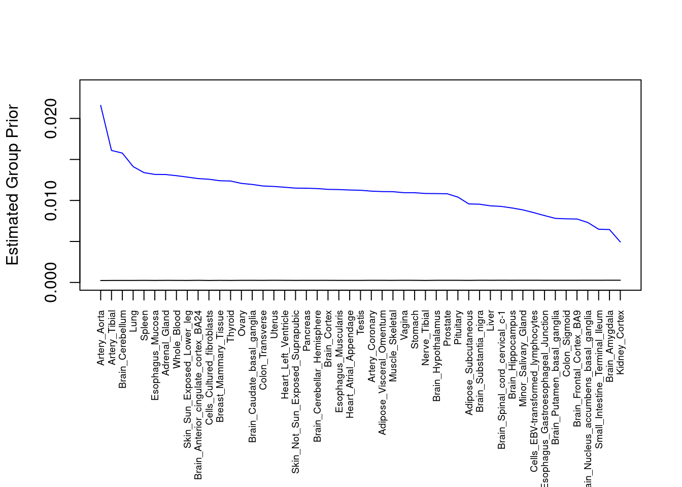
| Version | Author | Date |
|---|---|---|
| 4ded2ef | wesleycrouse | 2022-07-19 |
####################
#plot estimated group prior variance

par(mar=c(10.1, 4.1, 4.1, 2.1))

plot(output$prior_var_g, type="l", ylim=c(0, max(output$prior_var_g, output$prior_var_s)*1.1),
     xlab="", ylab="Estimated Group Prior Variance", xaxt = "n", col="blue")
lines(output$prior_var_s)

axis(1, at = 1:nrow(output),
     labels = output$weight,
     las=2,
     cex.axis=0.6)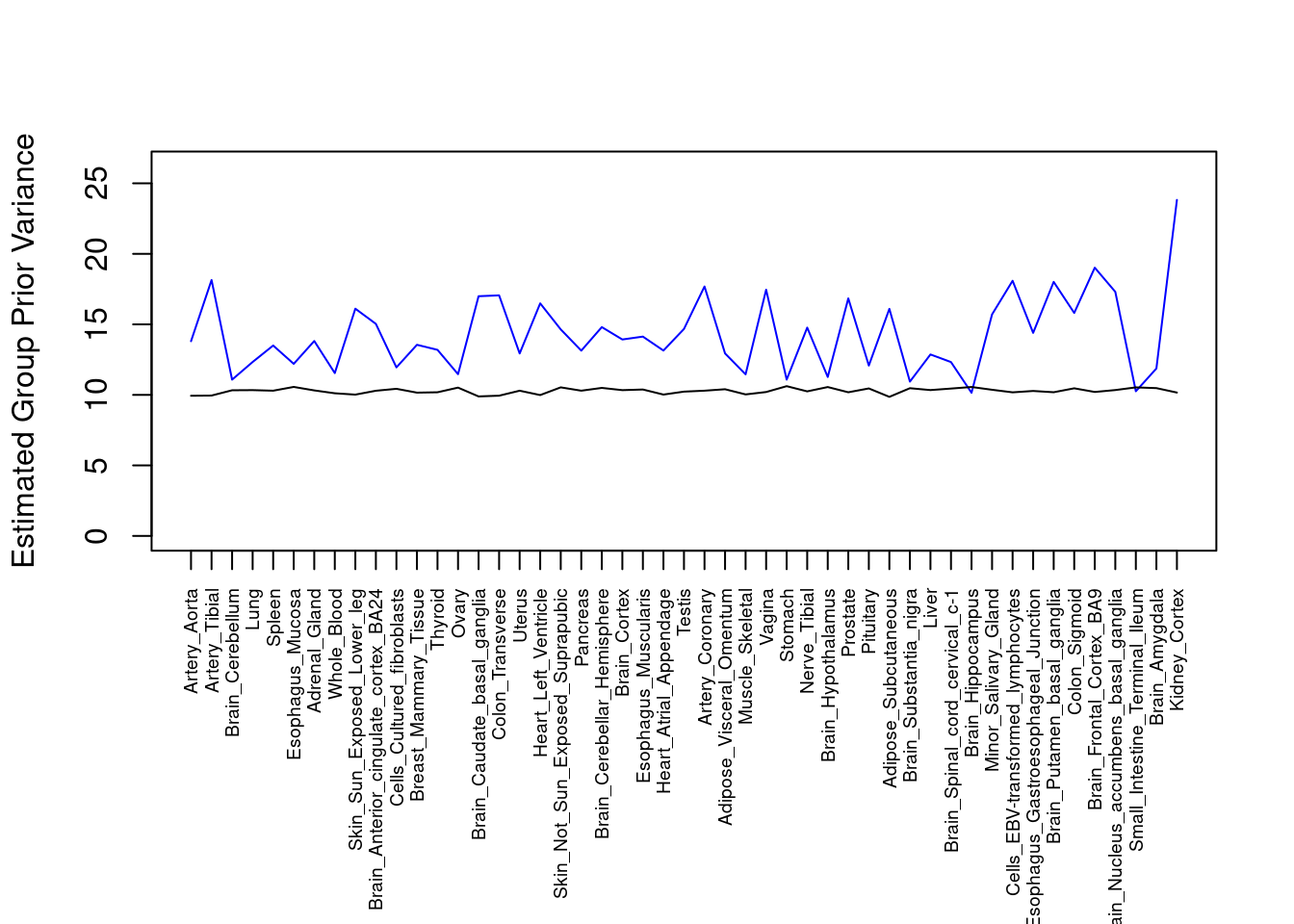
| Version | Author | Date |
|---|---|---|
| 4ded2ef | wesleycrouse | 2022-07-19 |
####################
#plot PVE

output <- output[order(-output$pve_g),]

par(mar=c(10.1, 4.1, 4.1, 2.1))

plot(output$pve_g, type="l", ylim=c(0, max(output$pve_g+output$pve_s)*1.1),
     xlab="", ylab="Estimated PVE", xaxt = "n", col="blue")
lines(output$pve_s)
lines(output$pve_g+output$pve_s, lty=2)

axis(1, at = 1:nrow(output),
     labels = output$weight,
     las=2,
     cex.axis=0.6)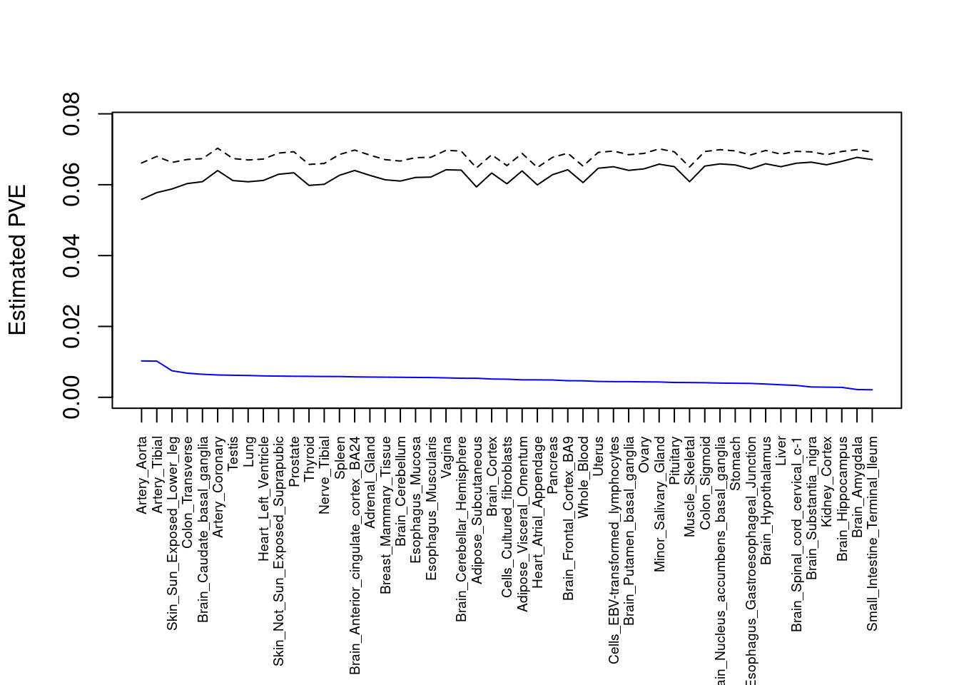
| Version | Author | Date |
|---|---|---|
| 4ded2ef | wesleycrouse | 2022-07-19 |
Number of cTWAS and TWAS genes
cTWAS genes are the set of genes with PIP>0.8 in any tissue. TWAS genes are the set of genes with significant z score (Bonferroni within tissue) in any tissue.
#plot number of significant cTWAS and TWAS genes in each tissue
plot(output$n_ctwas, output$n_twas, xlab="Number of cTWAS Genes", ylab="Number of TWAS Genes")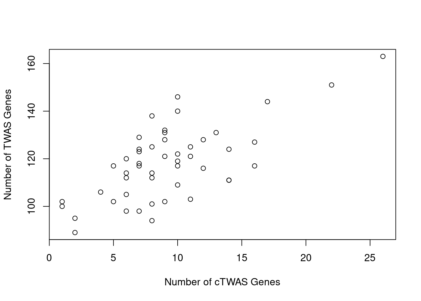
| Version | Author | Date |
|---|---|---|
| 4ded2ef | wesleycrouse | 2022-07-19 |
#number of ctwas_genes
ctwas_genes <- unique(unlist(lapply(df, function(x){x$ctwas})))
length(ctwas_genes)
[1] 142#number of twas_genes
twas_genes <- unique(unlist(lapply(df, function(x){x$twas})))
length(twas_genes)[1] 638Enrichment analysis for cTWAS genes
GO
#enrichment for cTWAS genes using enrichR
library(enrichR)
Welcome to enrichR
Checking connection ... Enrichr ... Connection is Live!
FlyEnrichr ... Connection is available!
WormEnrichr ... Connection is available!
YeastEnrichr ... Connection is available!
FishEnrichr ... Connection is available!dbs <- c("GO_Biological_Process_2021", "GO_Cellular_Component_2021", "GO_Molecular_Function_2021")
GO_enrichment <- enrichr(ctwas_genes, dbs)Uploading data to Enrichr... Done.
Querying GO_Biological_Process_2021... Done.
Querying GO_Cellular_Component_2021... Done.
Querying GO_Molecular_Function_2021... Done.
Parsing results... Done.for (db in dbs){
cat(paste0(db, "\n\n"))
enrich_results <- GO_enrichment[[db]]
enrich_results <- enrich_results[enrich_results$Adjusted.P.value<0.05,c("Term", "Overlap", "Adjusted.P.value", "Genes"), drop=F]
print(enrich_results)
print(plotEnrich(GO_enrichment[[db]]))
}GO_Biological_Process_2021
[1] Term Overlap Adjusted.P.value Genes
<0 rows> (or 0-length row.names)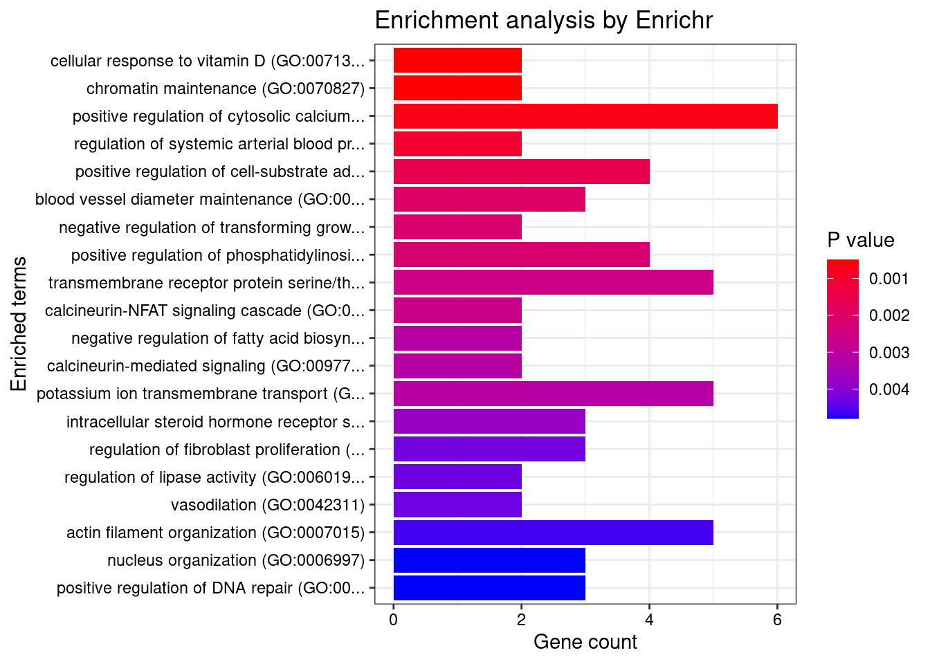
| Version | Author | Date |
|---|---|---|
| 4ded2ef | wesleycrouse | 2022-07-19 |
GO_Cellular_Component_2021
Term Overlap Adjusted.P.value Genes
1 cytoskeleton (GO:0005856) 13/600 0.04649444 RHOC;EML1;EFR3B;TRIOBP;LIMA1;MAEA;BIN1;FES;DLG4;STK38L;ZNF415;MYOZ1;MYO1F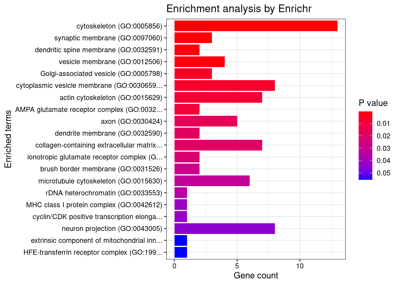
| Version | Author | Date |
|---|---|---|
| 4ded2ef | wesleycrouse | 2022-07-19 |
GO_Molecular_Function_2021
[1] Term Overlap Adjusted.P.value Genes
<0 rows> (or 0-length row.names)
| Version | Author | Date |
|---|---|---|
| 4ded2ef | wesleycrouse | 2022-07-19 |
KEGG
#enrichment for cTWAS genes using KEGG
library(WebGestaltR)******************************************* ** Welcome to WebGestaltR ! ** *******************************************background <- unique(unlist(lapply(df, function(x){x$gene_pips$genename})))
#listGeneSet()
databases <- c("pathway_KEGG")
enrichResult <- WebGestaltR(enrichMethod="ORA", organism="hsapiens",
interestGene=ctwas_genes, referenceGene=background,
enrichDatabase=databases, interestGeneType="genesymbol",
referenceGeneType="genesymbol", isOutput=F)Loading the functional categories...
Loading the ID list...
Loading the reference list...
Performing the enrichment analysis...Warning in oraEnrichment(interestGeneList, referenceGeneList, geneSet, minNum = minNum, : No significant gene set is identified based on FDR 0.05!enrichResult[,c("description", "size", "overlap", "FDR", "userId")]NULLDisGeNET
#enrichment for cTWAS genes using DisGeNET
# devtools::install_bitbucket("ibi_group/disgenet2r")
library(disgenet2r)
disgenet_api_key <- get_disgenet_api_key(
email = "wesleycrouse@gmail.com",
password = "uchicago1" )
Sys.setenv(DISGENET_API_KEY= disgenet_api_key)
res_enrich <- disease_enrichment(entities=ctwas_genes, vocabulary = "HGNC", database = "CURATED")
if (any(res_enrich@qresult$FDR < 0.05)){
print(res_enrich@qresult[res_enrich@qresult$FDR < 0.05, c("Description", "FDR", "Ratio", "BgRatio")])
}Gene sets curated by Macarthur Lab
gene_set_dir <- "/project2/mstephens/wcrouse/gene_sets/"
gene_set_files <- c("gwascatalog.tsv",
"mgi_essential.tsv",
"core_essentials_hart.tsv",
"clinvar_path_likelypath.tsv",
"fda_approved_drug_targets.tsv")
gene_sets <- lapply(gene_set_files, function(x){as.character(read.table(paste0(gene_set_dir, x))[,1])})
names(gene_sets) <- sapply(gene_set_files, function(x){unlist(strsplit(x, "[.]"))[1]})
gene_lists <- list(ctwas_genes=ctwas_genes)
#background is union of genes analyzed in all tissue
background <- unique(unlist(lapply(df, function(x){x$gene_pips$genename})))
#genes in gene_sets filtered to ensure inclusion in background
gene_sets <- lapply(gene_sets, function(x){x[x %in% background]})
####################
hyp_score <- data.frame()
size <- c()
ngenes <- c()
for (i in 1:length(gene_sets)) {
for (j in 1:length(gene_lists)){
group1 <- length(gene_sets[[i]])
group2 <- length(as.vector(gene_lists[[j]]))
size <- c(size, group1)
Overlap <- length(intersect(gene_sets[[i]],as.vector(gene_lists[[j]])))
ngenes <- c(ngenes, Overlap)
Total <- length(background)
hyp_score[i,j] <- phyper(Overlap-1, group2, Total-group2, group1,lower.tail=F)
}
}
rownames(hyp_score) <- names(gene_sets)
colnames(hyp_score) <- names(gene_lists)
hyp_score_padj <- apply(hyp_score,2, p.adjust, method="BH", n=(nrow(hyp_score)*ncol(hyp_score)))
hyp_score_padj <- as.data.frame(hyp_score_padj)
hyp_score_padj$gene_set <- rownames(hyp_score_padj)
hyp_score_padj$nset <- size
hyp_score_padj$ngenes <- ngenes
hyp_score_padj$percent <- ngenes/size
hyp_score_padj <- hyp_score_padj[order(hyp_score_padj$ctwas_genes),]
colnames(hyp_score_padj)[1] <- "padj"
hyp_score_padj <- hyp_score_padj[,c(2:5,1)]
rownames(hyp_score_padj)<- NULL
hyp_score_padj gene_set nset ngenes percent padj
1 gwascatalog 5957 76 0.012758100 1.963737e-05
2 mgi_essential 2299 25 0.010874293 1.593451e-01
3 fda_approved_drug_targets 350 6 0.017142857 1.593451e-01
4 core_essentials_hart 265 4 0.015094340 2.246808e-01
5 clinvar_path_likelypath 2766 26 0.009399855 2.792931e-01Enrichment analysis for TWAS genes
#enrichment for TWAS genes
dbs <- c("GO_Biological_Process_2021", "GO_Cellular_Component_2021", "GO_Molecular_Function_2021")
GO_enrichment <- enrichr(twas_genes, dbs)Uploading data to Enrichr... Done.
Querying GO_Biological_Process_2021... Done.
Querying GO_Cellular_Component_2021... Done.
Querying GO_Molecular_Function_2021... Done.
Parsing results... Done.for (db in dbs){
cat(paste0(db, "\n\n"))
enrich_results <- GO_enrichment[[db]]
enrich_results <- enrich_results[enrich_results$Adjusted.P.value<0.05,c("Term", "Overlap", "Adjusted.P.value", "Genes")]
print(enrich_results)
print(plotEnrich(GO_enrichment[[db]]))
}GO_Biological_Process_2021
Term Overlap Adjusted.P.value Genes
1 cellular senescence (GO:0090398) 7/27 0.03270837 SPI1;PRKCD;ULK3;MAPKAPK5;SIRT1;TBX3;TBX2
2 positive regulation of microtubule polymerization (GO:0031116) 7/28 0.03270837 FES;AKAP9;SLAIN2;MAPT;HSPA1B;CDK5R1;HSPA1A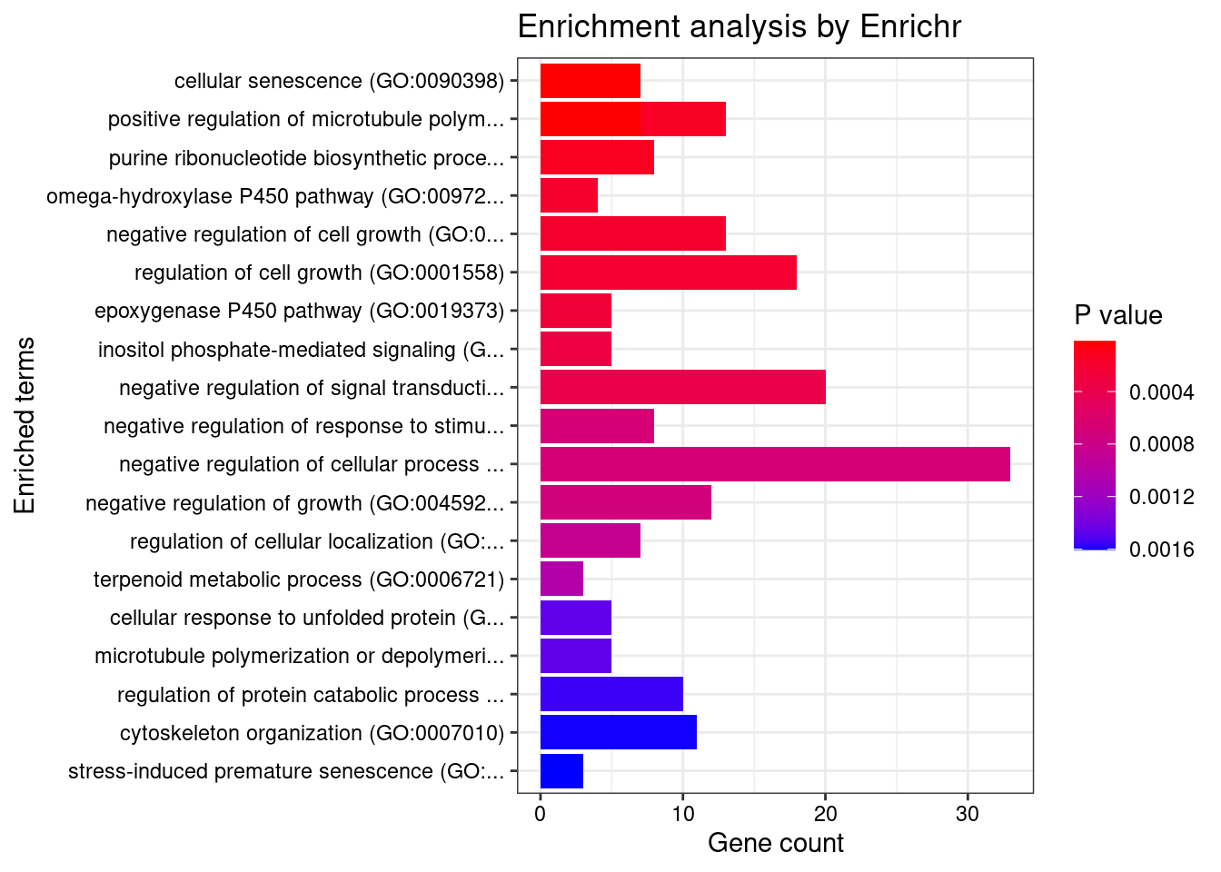
GO_Cellular_Component_2021
[1] Term Overlap Adjusted.P.value Genes
<0 rows> (or 0-length row.names)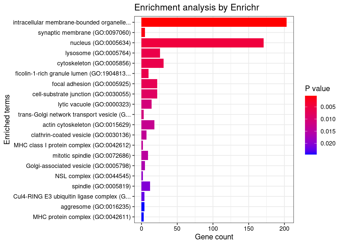
GO_Molecular_Function_2021
[1] Term Overlap Adjusted.P.value Genes
<0 rows> (or 0-length row.names)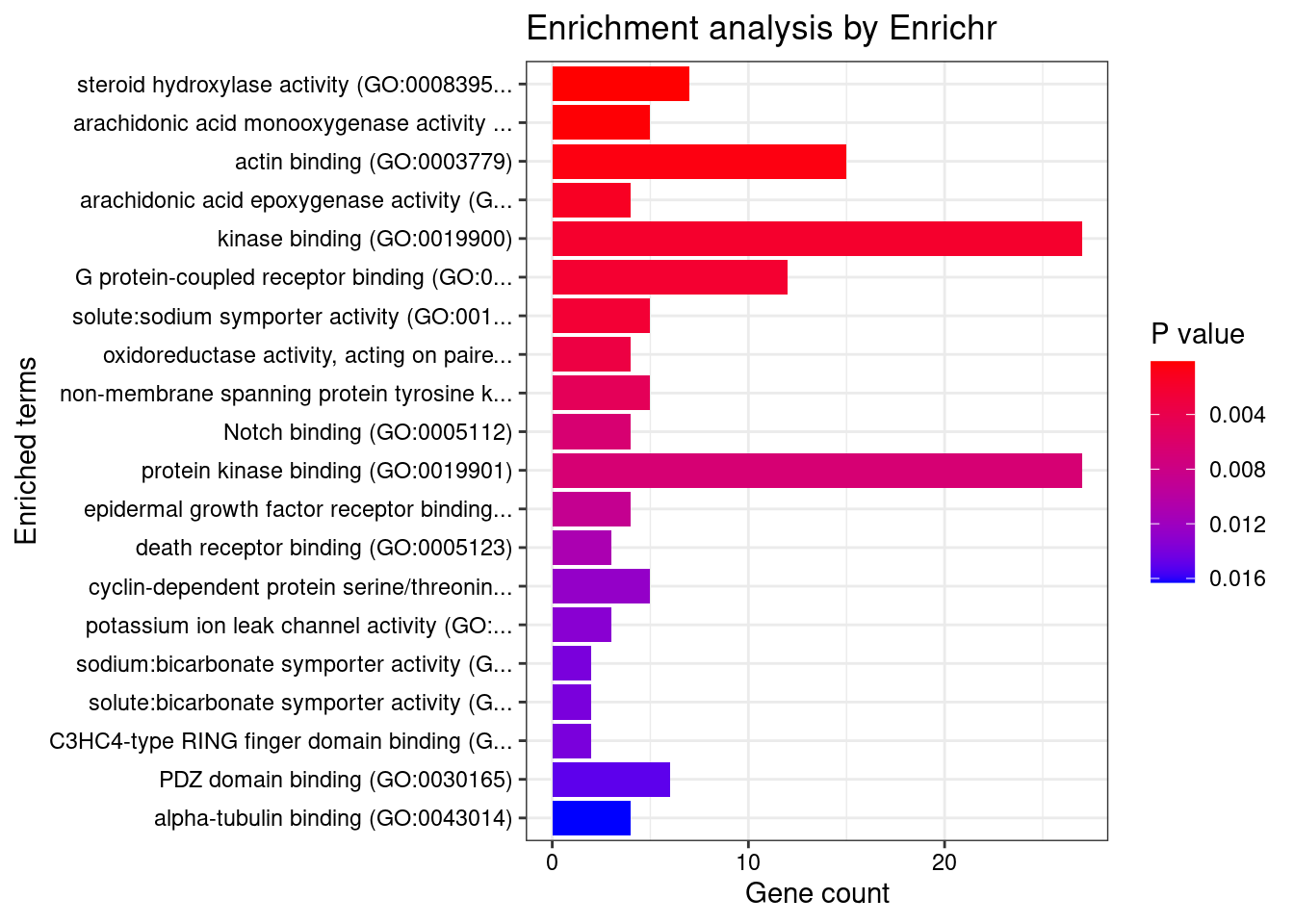
Enrichment analysis for cTWAS genes in top tissues separately
GO
output <- output[order(-output$pve_g),]
top_tissues <- output$weight[1:5]
for (tissue in top_tissues){
cat(paste0(tissue, "\n\n"))
ctwas_genes_tissue <- df[[tissue]]$ctwas
cat(paste0("Number of cTWAS Genes in Tissue: ", length(ctwas_genes_tissue), "\n\n"))
dbs <- c("GO_Biological_Process_2021")
GO_enrichment <- enrichr(ctwas_genes_tissue, dbs)
for (db in dbs){
cat(paste0("\n", db, "\n\n"))
enrich_results <- GO_enrichment[[db]]
enrich_results <- enrich_results[enrich_results$Adjusted.P.value<0.05,c("Term", "Overlap", "Adjusted.P.value", "Genes")]
print(enrich_results)
print(plotEnrich(GO_enrichment[[db]]))
}
}Artery_Aorta
Number of cTWAS Genes in Tissue: 22
Uploading data to Enrichr... Done.
Querying GO_Biological_Process_2021... Done.
Parsing results... Done.
GO_Biological_Process_2021
Term Overlap Adjusted.P.value Genes
1 positive regulation of phosphatidylinositol 3-kinase signaling (GO:0014068) 3/77 0.03903628 GPER1;FN1;SIRT1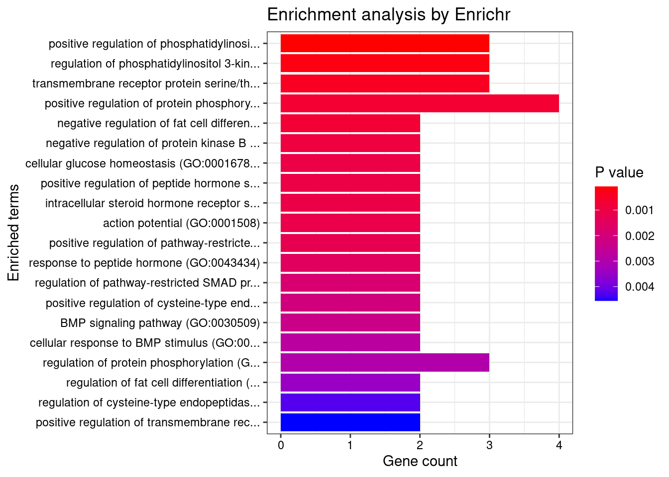
| Version | Author | Date |
|---|---|---|
| 4ded2ef | wesleycrouse | 2022-07-19 |
Artery_Tibial
Number of cTWAS Genes in Tissue: 26
Uploading data to Enrichr... Done.
Querying GO_Biological_Process_2021... Done.
Parsing results... Done.
GO_Biological_Process_2021
Term Overlap Adjusted.P.value Genes
1 stress fiber assembly (GO:0043149) 2/15 0.02313407 ITGB5;PHACTR1
2 contractile actin filament bundle assembly (GO:0030038) 2/15 0.02313407 ITGB5;PHACTR1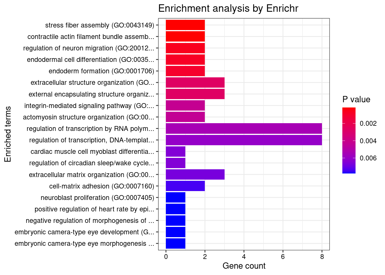
| Version | Author | Date |
|---|---|---|
| 4ded2ef | wesleycrouse | 2022-07-19 |
Skin_Sun_Exposed_Lower_leg
Number of cTWAS Genes in Tissue: 17
Uploading data to Enrichr... Done.
Querying GO_Biological_Process_2021... Done.
Parsing results... Done.
GO_Biological_Process_2021
Term Overlap Adjusted.P.value Genes
1 potassium ion transmembrane transport (GO:0071805) 3/139 0.0345271 KCNQ5;ATP12A;KCNK3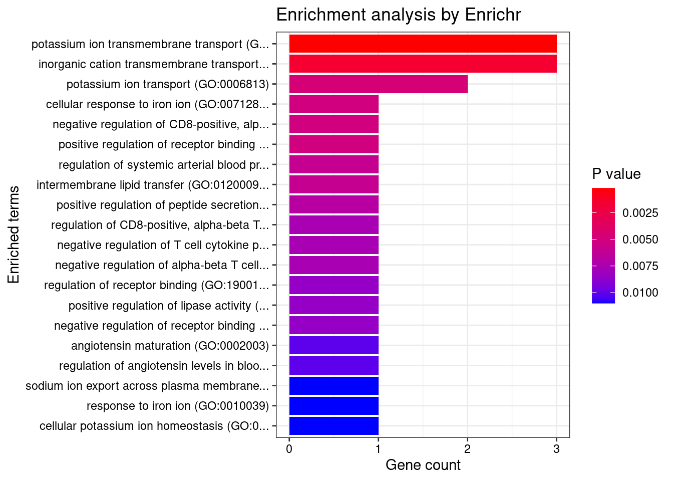
| Version | Author | Date |
|---|---|---|
| 4ded2ef | wesleycrouse | 2022-07-19 |
Colon_Transverse
Number of cTWAS Genes in Tissue: 9
Uploading data to Enrichr... Done.
Querying GO_Biological_Process_2021... Done.
Parsing results... Done.
GO_Biological_Process_2021

[1] Term             Overlap          Adjusted.P.value Genes
<0 rows> (or 0-length row.names)
| Version | Author | Date |
|---|---|---|
| 4ded2ef | wesleycrouse | 2022-07-19 |
Brain_Caudate_basal_ganglia
Number of cTWAS Genes in Tissue: 10
Uploading data to Enrichr... Done.
Querying GO_Biological_Process_2021... Done.
Parsing results... Done.
GO_Biological_Process_2021
[1] Term Overlap Adjusted.P.value Genes
<0 rows> (or 0-length row.names)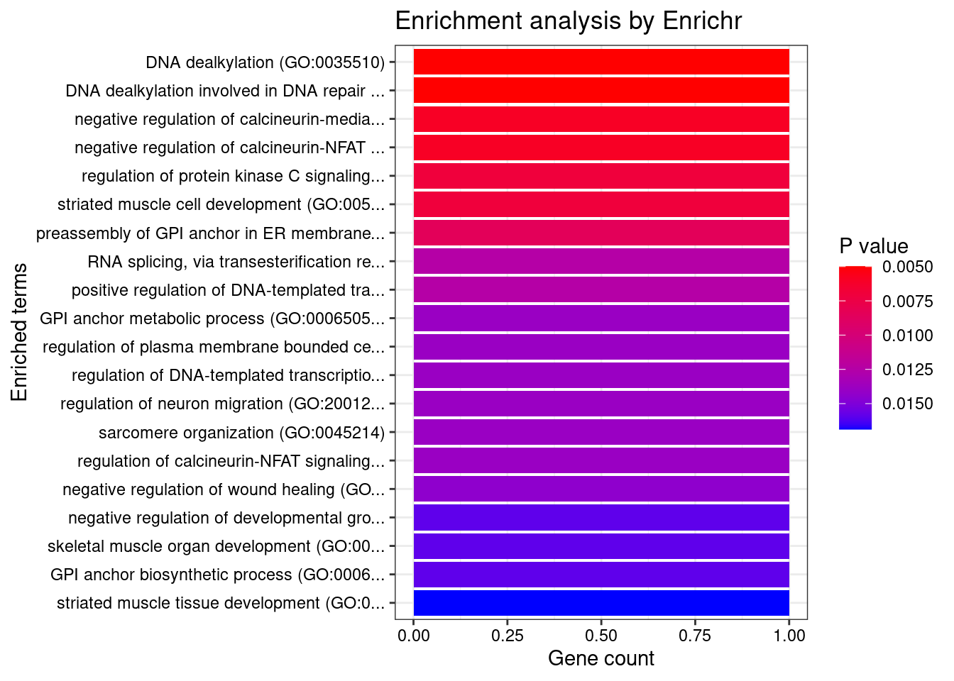
| Version | Author | Date |
|---|---|---|
| 4ded2ef | wesleycrouse | 2022-07-19 |
KEGG
output <- output[order(-output$pve_g),]
top_tissues <- output$weight[1:5]
for (tissue in top_tissues){
cat(paste0(tissue, "\n\n"))
ctwas_genes_tissue <- df[[tissue]]$ctwas
background_tissue <- df[[tissue]]$gene_pips$genename
cat(paste0("Number of cTWAS Genes in Tissue: ", length(ctwas_genes_tissue), "\n\n"))
databases <- c("pathway_KEGG")
enrichResult <- NULL
try(enrichResult <- WebGestaltR(enrichMethod="ORA", organism="hsapiens",
interestGene=ctwas_genes_tissue, referenceGene=background_tissue,
enrichDatabase=databases, interestGeneType="genesymbol",
referenceGeneType="genesymbol", isOutput=F))
if (!is.null(enrichResult)){
print(enrichResult[,c("description", "size", "overlap", "FDR", "userId")])
}
cat("\n")
} Artery_Aorta
Number of cTWAS Genes in Tissue: 22
Loading the functional categories...
Loading the ID list...
Loading the reference list...
Performing the enrichment analysis...
Warning in oraEnrichment(interestGeneList, referenceGeneList, geneSet, minNum = minNum, : No significant gene set is identified based on FDR 0.05!
Artery_Tibial

Number of cTWAS Genes in Tissue: 26

Loading the functional categories...
Loading the ID list...
Loading the reference list...
Performing the enrichment analysis...
Warning in oraEnrichment(interestGeneList, referenceGeneList, geneSet, minNum = minNum, : No significant gene set is identified based on FDR 0.05!
Skin_Sun_Exposed_Lower_leg

Number of cTWAS Genes in Tissue: 17

Loading the functional categories...
Loading the ID list...
Loading the reference list...
Performing the enrichment analysis...
Warning in oraEnrichment(interestGeneList, referenceGeneList, geneSet, minNum = minNum, : No significant gene set is identified based on FDR 0.05!
Colon_Transverse

Number of cTWAS Genes in Tissue: 9

Loading the functional categories...
Loading the ID list...
Loading the reference list...
Performing the enrichment analysis...
Warning in oraEnrichment(interestGeneList, referenceGeneList, geneSet, minNum = minNum, : No significant gene set is identified based on FDR 0.05!
Brain_Caudate_basal_ganglia

Number of cTWAS Genes in Tissue: 10

Loading the functional categories...
Loading the ID list...
Loading the reference list...
Performing the enrichment analysis...
Warning in oraEnrichment(interestGeneList, referenceGeneList, geneSet, minNum = minNum, : No significant gene set is identified based on FDR 0.05!DisGeNET
output <- output[order(-output$pve_g),]
top_tissues <- output$weight[1:5]

for (tissue in top_tissues){
  cat(paste0(tissue, "\n\n"))

  ctwas_genes_tissue <- df[[tissue]]$ctwas

  cat(paste0("Number of cTWAS Genes in Tissue: ", length(ctwas_genes_tissue), "\n\n"))

  res_enrich <- disease_enrichment(entities=ctwas_genes_tissue, vocabulary = "HGNC", database = "CURATED")

  if (any(res_enrich@qresult$FDR < 0.05)){
    print(res_enrich@qresult[res_enrich@qresult$FDR < 0.05, c("Description", "FDR", "Ratio",  "BgRatio")])
  }

  cat("\n")
}
Gene sets curated by Macarthur Lab
output <- output[order(-output$pve_g),]
top_tissues <- output$weight[1:5]

gene_set_dir <- "/project2/mstephens/wcrouse/gene_sets/"
gene_set_files <- c("gwascatalog.tsv",
                    "mgi_essential.tsv",
                    "core_essentials_hart.tsv",
                    "clinvar_path_likelypath.tsv",
                    "fda_approved_drug_targets.tsv")

for (tissue in top_tissues){
  cat(paste0(tissue, "\n\n"))

  ctwas_genes_tissue <- df[[tissue]]$ctwas
  background_tissue <- df[[tissue]]$gene_pips$genename

  cat(paste0("Number of cTWAS Genes in Tissue: ", length(ctwas_genes_tissue), "\n\n"))

  gene_sets <- lapply(gene_set_files, function(x){as.character(read.table(paste0(gene_set_dir, x))[,1])})
  names(gene_sets) <- sapply(gene_set_files, function(x){unlist(strsplit(x, "[.]"))[1]})

  gene_lists <- list(ctwas_genes_tissue=ctwas_genes_tissue)

  #genes in gene_sets filtered to ensure inclusion in background
  gene_sets <- lapply(gene_sets, function(x){x[x %in% background_tissue]})

  ##########
  hyp_score <- data.frame()
  size <- c()
  ngenes <- c()

  for (i in 1:length(gene_sets)) {
    for (j in 1:length(gene_lists)){
      group1 <- length(gene_sets[[i]])
      group2 <- length(as.vector(gene_lists[[j]]))
      size <- c(size, group1)
      Overlap <- length(intersect(gene_sets[[i]],as.vector(gene_lists[[j]])))
      ngenes <- c(ngenes, Overlap)
      Total <- length(background_tissue)
      hyp_score[i,j] <- phyper(Overlap-1, group2, Total-group2, group1,lower.tail=F)
    }
  }
  rownames(hyp_score) <- names(gene_sets)
  colnames(hyp_score) <- names(gene_lists)

  hyp_score_padj <- apply(hyp_score,2, p.adjust, method="BH", n=(nrow(hyp_score)*ncol(hyp_score)))
  hyp_score_padj <- as.data.frame(hyp_score_padj)
  hyp_score_padj$gene_set <- rownames(hyp_score_padj)
  hyp_score_padj$nset <- size
  hyp_score_padj$ngenes <- ngenes
  hyp_score_padj$percent <- ngenes/size

  hyp_score_padj <- hyp_score_padj[order(hyp_score_padj$ctwas_genes),]
  colnames(hyp_score_padj)[1] <- "padj"
  hyp_score_padj <- hyp_score_padj[,c(2:5,1)]
  rownames(hyp_score_padj)<- NULL

  print(hyp_score_padj)

  cat("\n")
}
Artery_Aorta
Number of cTWAS Genes in Tissue: 22
gene_set nset ngenes percent padj
1 mgi_essential 1443 6 0.004158004 0.3001662
2 gwascatalog 3877 9 0.002321383 0.4617251
3 clinvar_path_likelypath 1814 5 0.002756340 0.4617251
4 fda_approved_drug_targets 203 1 0.004926108 0.4617251
5 core_essentials_hart 180 0 0.000000000 1.0000000
Artery_Tibial
Number of cTWAS Genes in Tissue: 26
gene_set nset ngenes percent padj
1 gwascatalog 3920 18 0.004591837 0.002201663
2 fda_approved_drug_targets 206 3 0.014563107 0.029884810
3 mgi_essential 1468 6 0.004087193 0.166118236
4 clinvar_path_likelypath 1865 7 0.003753351 0.166118236
5 core_essentials_hart 193 1 0.005181347 0.366493006
Skin_Sun_Exposed_Lower_leg
Number of cTWAS Genes in Tissue: 17
gene_set nset ngenes percent padj
1 gwascatalog 4060 11 0.002709360 0.06465674
2 core_essentials_hart 199 1 0.005025126 0.46343211
3 fda_approved_drug_targets 218 1 0.004587156 0.46343211
4 mgi_essential 1511 3 0.001985440 0.48865035
5 clinvar_path_likelypath 1912 3 0.001569038 0.55532561
Colon_Transverse
Number of cTWAS Genes in Tissue: 9
gene_set nset ngenes percent padj
1 gwascatalog 3776 8 0.0021186441 0.00699829
2 mgi_essential 1392 3 0.0021551724 0.24815428
3 core_essentials_hart 186 0 0.0000000000 1.00000000
4 clinvar_path_likelypath 1782 1 0.0005611672 1.00000000
5 fda_approved_drug_targets 197 0 0.0000000000 1.00000000
Brain_Caudate_basal_ganglia
Number of cTWAS Genes in Tissue: 10
gene_set nset ngenes percent padj
1 gwascatalog 3541 5 0.0014120305 0.6129543
2 core_essentials_hart 181 1 0.0055248619 0.6129543
3 mgi_essential 1306 1 0.0007656968 1.0000000
4 clinvar_path_likelypath 1673 1 0.0005977286 1.0000000
5 fda_approved_drug_targets 174 0 0.0000000000 1.0000000Summary of results across tissues
weight_groups <- as.data.frame(matrix(c("Adipose_Subcutaneous", "Adipose",
                                        "Adipose_Visceral_Omentum", "Adipose",
                                        "Adrenal_Gland", "Endocrine",
                                        "Artery_Aorta", "Cardiovascular",
                                        "Artery_Coronary", "Cardiovascular",
                                        "Artery_Tibial", "Cardiovascular",
                                        "Brain_Amygdala", "CNS",
                                        "Brain_Anterior_cingulate_cortex_BA24", "CNS",
                                        "Brain_Caudate_basal_ganglia", "CNS",
                                        "Brain_Cerebellar_Hemisphere", "CNS",
                                        "Brain_Cerebellum", "CNS",
                                        "Brain_Cortex", "CNS",
                                        "Brain_Frontal_Cortex_BA9", "CNS",
                                        "Brain_Hippocampus", "CNS",
                                        "Brain_Hypothalamus", "CNS",
                                        "Brain_Nucleus_accumbens_basal_ganglia", "CNS",
                                        "Brain_Putamen_basal_ganglia", "CNS",
                                        "Brain_Spinal_cord_cervical_c-1", "CNS",
                                        "Brain_Substantia_nigra", "CNS",
                                        "Breast_Mammary_Tissue", "None",
                                        "Cells_Cultured_fibroblasts", "Skin",
                                        "Cells_EBV-transformed_lymphocytes", "Blood or Immune",
                                        "Colon_Sigmoid", "Digestive",
                                        "Colon_Transverse", "Digestive",
                                        "Esophagus_Gastroesophageal_Junction", "Digestive",
                                        "Esophagus_Mucosa", "Digestive",
                                        "Esophagus_Muscularis", "Digestive",
                                        "Heart_Atrial_Appendage", "Cardiovascular",
                                        "Heart_Left_Ventricle", "Cardiovascular",
                                        "Kidney_Cortex", "None",
                                        "Liver", "None",
                                        "Lung", "None",
                                        "Minor_Salivary_Gland", "None",
                                        "Muscle_Skeletal", "None",
                                        "Nerve_Tibial", "None",
                                        "Ovary", "None",
                                        "Pancreas", "None",
                                        "Pituitary", "Endocrine",
                                        "Prostate", "None",
                                        "Skin_Not_Sun_Exposed_Suprapubic", "Skin",
                                        "Skin_Sun_Exposed_Lower_leg", "Skin",
                                        "Small_Intestine_Terminal_Ileum", "Digestive",
                                        "Spleen", "Blood or Immune",
                                        "Stomach", "Digestive",
                                        "Testis", "Endocrine",
                                        "Thyroid", "Endocrine",
                                        "Uterus", "None",
                                        "Vagina", "None",
                                        "Whole_Blood", "Blood or Immune"),
                                      nrow=49, ncol=2, byrow=T), stringsAsFactors=F)
colnames(weight_groups) <- c("weight", "group")

#display tissue groups
print(weight_groups)
weight group
1 Adipose_Subcutaneous Adipose
2 Adipose_Visceral_Omentum Adipose
3 Adrenal_Gland Endocrine
4 Artery_Aorta Cardiovascular
5 Artery_Coronary Cardiovascular
6 Artery_Tibial Cardiovascular
7 Brain_Amygdala CNS
8 Brain_Anterior_cingulate_cortex_BA24 CNS
9 Brain_Caudate_basal_ganglia CNS
10 Brain_Cerebellar_Hemisphere CNS
11 Brain_Cerebellum CNS
12 Brain_Cortex CNS
13 Brain_Frontal_Cortex_BA9 CNS
14 Brain_Hippocampus CNS
15 Brain_Hypothalamus CNS
16 Brain_Nucleus_accumbens_basal_ganglia CNS
17 Brain_Putamen_basal_ganglia CNS
18 Brain_Spinal_cord_cervical_c-1 CNS
19 Brain_Substantia_nigra CNS
20 Breast_Mammary_Tissue None
21 Cells_Cultured_fibroblasts Skin
22 Cells_EBV-transformed_lymphocytes Blood or Immune
23 Colon_Sigmoid Digestive
24 Colon_Transverse Digestive
25 Esophagus_Gastroesophageal_Junction Digestive
26 Esophagus_Mucosa Digestive
27 Esophagus_Muscularis Digestive
28 Heart_Atrial_Appendage Cardiovascular
29 Heart_Left_Ventricle Cardiovascular
30 Kidney_Cortex None
31 Liver None
32 Lung None
33 Minor_Salivary_Gland None
34 Muscle_Skeletal None
35 Nerve_Tibial None
36 Ovary None
37 Pancreas None
38 Pituitary Endocrine
39 Prostate None
40 Skin_Not_Sun_Exposed_Suprapubic Skin
41 Skin_Sun_Exposed_Lower_leg Skin
42 Small_Intestine_Terminal_Ileum Digestive
43 Spleen Blood or Immune
44 Stomach Digestive
45 Testis Endocrine
46 Thyroid Endocrine
47 Uterus None
48 Vagina None
49 Whole_Blood Blood or Immunegroups <- unique(weight_groups$group)
df_group <- list()
for (i in 1:length(groups)){
group <- groups[i]
weights <- weight_groups$weight[weight_groups$group==group]
df_group[[group]] <- list(ctwas=unique(unlist(lapply(df[weights], function(x){x$ctwas}))),
background=unique(unlist(lapply(df[weights], function(x){x$gene_pips$genename}))))
}
output <- output[sapply(weight_groups$weight, match, output$weight),,drop=F]
output$group <- weight_groups$group
output$n_ctwas_group <- sapply(output$group, function(x){length(df_group[[x]][["ctwas"]])})
output$n_ctwas_group[output$group=="None"] <- 0
#barplot of number of cTWAS genes in each tissue
output <- output[order(-output$n_ctwas),,drop=F]
par(mar=c(10.1, 4.1, 4.1, 2.1))
barplot(output$n_ctwas, names.arg=output$weight, las=2, ylab="Number of cTWAS Genes", cex.names=0.6, main="Number of cTWAS Genes by Tissue")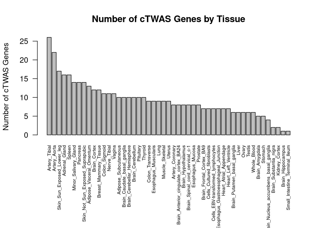
| Version | Author | Date |
|---|---|---|
| 4ded2ef | wesleycrouse | 2022-07-19 |
#barplot of number of cTWAS genes in each tissue
df_plot <- -sort(-sapply(groups[groups!="None"], function(x){length(df_group[[x]][["ctwas"]])}))

par(mar=c(10.1, 4.1, 4.1, 2.1))
barplot(df_plot, las=2, ylab="Number of cTWAS Genes", main="Number of cTWAS Genes by Tissue Group")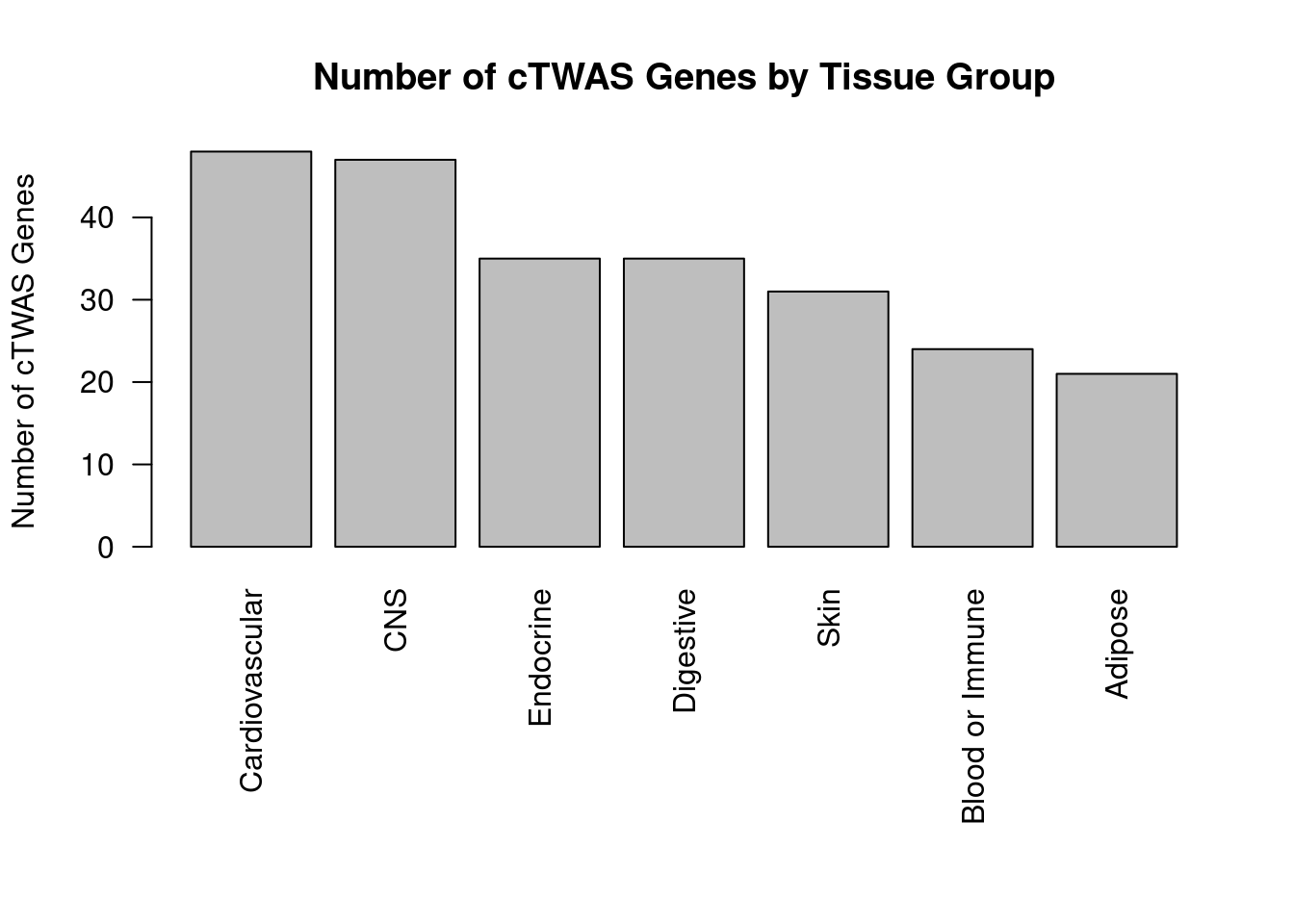
| Version | Author | Date |
|---|---|---|
| 4ded2ef | wesleycrouse | 2022-07-19 |
Enrichment analysis for cTWAS genes in each tissue group
GO
suppressWarnings(rm(group_enrichment_results))

for (group in names(df_group)){
  cat(paste0(group, "\n\n"))

  ctwas_genes_group <- df_group[[group]]$ctwas

  cat(paste0("Number of cTWAS Genes in Tissue Group: ", length(ctwas_genes_group), "\n\n"))

  dbs <- c("GO_Biological_Process_2021")
  GO_enrichment <- enrichr(ctwas_genes_group, dbs)

  for (db in dbs){
    cat(paste0("\n", db, "\n\n"))
    enrich_results <- GO_enrichment[[db]]
    enrich_results <- enrich_results[enrich_results$Adjusted.P.value<0.05,c("Term", "Overlap", "Adjusted.P.value", "Genes")]
    print(enrich_results)
    print(plotEnrich(GO_enrichment[[db]]))

    if (nrow(enrich_results)>0){
      if (!exists("group_enrichment_results")){
        group_enrichment_results <- cbind(group, db, enrich_results)
      } else {
        group_enrichment_results <- rbind(group_enrichment_results, cbind(group, db, enrich_results))
      }
    }
  }

}
Adipose
Number of cTWAS Genes in Tissue Group: 21
Uploading data to Enrichr... Done.
Querying GO_Biological_Process_2021... Done.
Parsing results... Done.
GO_Biological_Process_2021
[1] Term Overlap Adjusted.P.value Genes
<0 rows> (or 0-length row.names)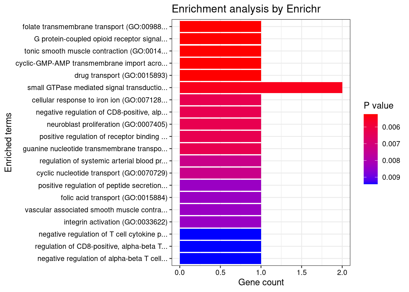
| Version | Author | Date |
|---|---|---|
| 4ded2ef | wesleycrouse | 2022-07-19 |
Endocrine

Number of cTWAS Genes in Tissue Group: 35

Uploading data to Enrichr... Done.
  Querying GO_Biological_Process_2021... Done.
Parsing results... Done.

GO_Biological_Process_2021

[1] Term             Overlap          Adjusted.P.value Genes
<0 rows> (or 0-length row.names)
| Version | Author | Date |
|---|---|---|
| 4ded2ef | wesleycrouse | 2022-07-19 |
Cardiovascular

Number of cTWAS Genes in Tissue Group: 48

Uploading data to Enrichr... Done.
  Querying GO_Biological_Process_2021... Done.
Parsing results... Done.

GO_Biological_Process_2021

[1] Term             Overlap          Adjusted.P.value Genes
<0 rows> (or 0-length row.names)
| Version | Author | Date |
|---|---|---|
| 4ded2ef | wesleycrouse | 2022-07-19 |
CNS

Number of cTWAS Genes in Tissue Group: 47

Uploading data to Enrichr... Done.
  Querying GO_Biological_Process_2021... Done.
Parsing results... Done.

GO_Biological_Process_2021

[1] Term             Overlap          Adjusted.P.value Genes
<0 rows> (or 0-length row.names)
| Version | Author | Date |
|---|---|---|
| 4ded2ef | wesleycrouse | 2022-07-19 |
None

Number of cTWAS Genes in Tissue Group: 59

Uploading data to Enrichr... Done.
  Querying GO_Biological_Process_2021... Done.
Parsing results... Done.

GO_Biological_Process_2021

[1] Term             Overlap          Adjusted.P.value Genes
<0 rows> (or 0-length row.names)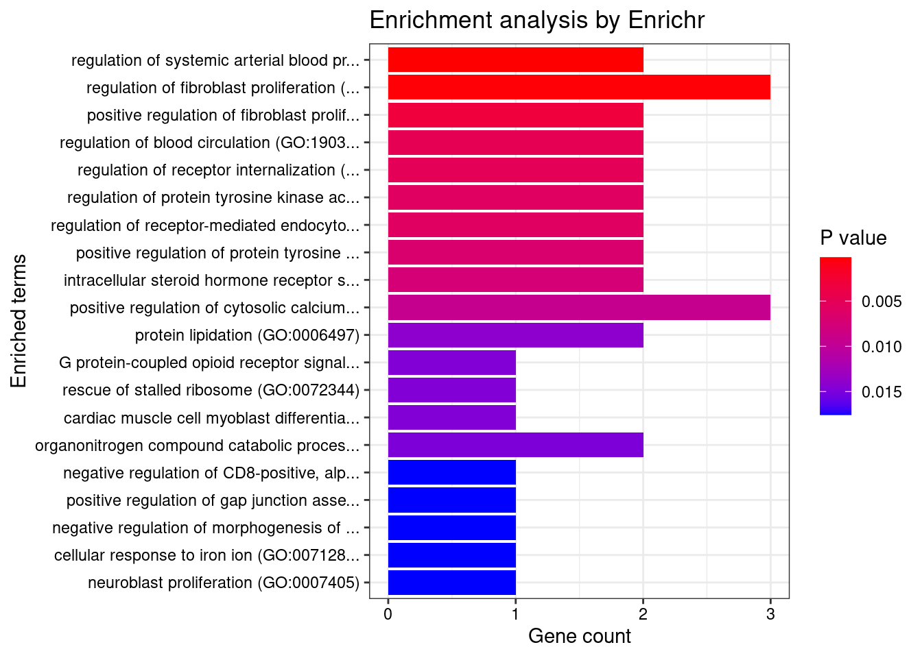
| Version | Author | Date |
|---|---|---|
| 4ded2ef | wesleycrouse | 2022-07-19 |
Skin

Number of cTWAS Genes in Tissue Group: 31

Uploading data to Enrichr... Done.
  Querying GO_Biological_Process_2021... Done.
Parsing results... Done.

GO_Biological_Process_2021

[1] Term             Overlap          Adjusted.P.value Genes
<0 rows> (or 0-length row.names)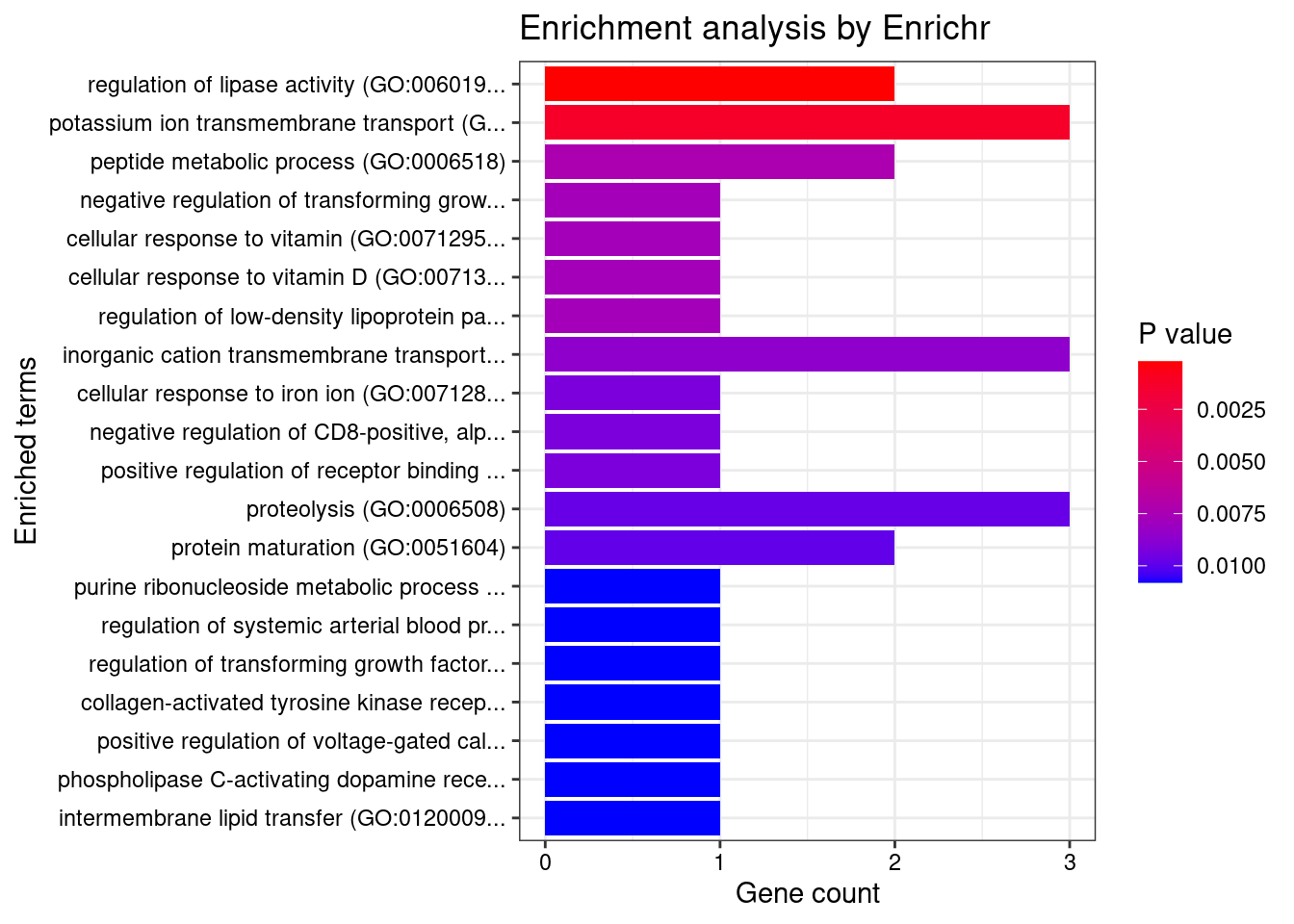
| Version | Author | Date |
|---|---|---|
| 4ded2ef | wesleycrouse | 2022-07-19 |
Blood or Immune

Number of cTWAS Genes in Tissue Group: 24

Uploading data to Enrichr... Done.
  Querying GO_Biological_Process_2021... Done.
Parsing results... Done.

GO_Biological_Process_2021

                                                                              Term Overlap Adjusted.P.value         Genes
1                              regulation of fibroblast proliferation (GO:0048145)    3/46      0.005283911 MORC3;FN1;AGT
2 regulation of systemic arterial blood pressure by renin-angiotensin (GO:0003081)     2/7      0.005283911     ENPEP;AGT
| Version | Author | Date |
|---|---|---|
| 4ded2ef | wesleycrouse | 2022-07-19 |
Digestive

Number of cTWAS Genes in Tissue Group: 35

Uploading data to Enrichr... Done.
  Querying GO_Biological_Process_2021... Done.
Parsing results... Done.

GO_Biological_Process_2021

[1] Term             Overlap          Adjusted.P.value Genes
<0 rows> (or 0-length row.names)
| Version | Author | Date |
|---|---|---|
| 4ded2ef | wesleycrouse | 2022-07-19 |
if (exists("group_enrichment_results")){
  save(group_enrichment_results, file=paste0("group_enrichment_results_", trait_id, ".RData"))
}
KEGG
for (group in names(df_group)){
  cat(paste0(group, "\n\n"))

  ctwas_genes_group <- df_group[[group]]$ctwas
  background_group <- df_group[[group]]$background

  cat(paste0("Number of cTWAS Genes in Tissue Group: ", length(ctwas_genes_group), "\n\n"))

  databases <- c("pathway_KEGG")

  enrichResult <- WebGestaltR(enrichMethod="ORA", organism="hsapiens",
                              interestGene=ctwas_genes_group, referenceGene=background_group,
                              enrichDatabase=databases, interestGeneType="genesymbol",
                              referenceGeneType="genesymbol", isOutput=F)

  if (!is.null(enrichResult)){
    print(enrichResult[,c("description", "size", "overlap", "FDR", "userId")])
  }

  cat("\n")
}
Adipose
Number of cTWAS Genes in Tissue Group: 21
Loading the functional categories...
Loading the ID list...
Loading the reference list...
Performing the enrichment analysis...Warning in oraEnrichment(interestGeneList, referenceGeneList, geneSet, minNum = minNum, : No significant gene set is identified based on FDR 0.05!
Endocrine

Number of cTWAS Genes in Tissue Group: 35

Loading the functional categories...
Loading the ID list...
Loading the reference list...
Performing the enrichment analysis...
Warning in oraEnrichment(interestGeneList, referenceGeneList, geneSet, minNum = minNum, : No significant gene set is identified based on FDR 0.05!
Cardiovascular

Number of cTWAS Genes in Tissue Group: 48

Loading the functional categories...
Loading the ID list...
Loading the reference list...
Performing the enrichment analysis...
Warning in oraEnrichment(interestGeneList, referenceGeneList, geneSet, minNum = minNum, : No significant gene set is identified based on FDR 0.05!
CNS

Number of cTWAS Genes in Tissue Group: 47

Loading the functional categories...
Loading the ID list...
Loading the reference list...
Performing the enrichment analysis...
Warning in oraEnrichment(interestGeneList, referenceGeneList, geneSet, minNum = minNum, : No significant gene set is identified based on FDR 0.05!
None

Number of cTWAS Genes in Tissue Group: 59

Loading the functional categories...
Loading the ID list...
Loading the reference list...
Performing the enrichment analysis...
Warning in oraEnrichment(interestGeneList, referenceGeneList, geneSet, minNum = minNum, : No significant gene set is identified based on FDR 0.05!
Skin

Number of cTWAS Genes in Tissue Group: 31

Loading the functional categories...
Loading the ID list...
Loading the reference list...
Performing the enrichment analysis...
Warning in oraEnrichment(interestGeneList, referenceGeneList, geneSet, minNum = minNum, : No significant gene set is identified based on FDR 0.05!
Blood or Immune

Number of cTWAS Genes in Tissue Group: 24

Loading the functional categories...
Loading the ID list...
Loading the reference list...
Performing the enrichment analysis...
Warning in oraEnrichment(interestGeneList, referenceGeneList, geneSet, minNum = minNum, : No significant gene set is identified based on FDR 0.05!
Digestive

Number of cTWAS Genes in Tissue Group: 35

Loading the functional categories...
Loading the ID list...
Loading the reference list...
Performing the enrichment analysis...
Warning in oraEnrichment(interestGeneList, referenceGeneList, geneSet, minNum = minNum, : No significant gene set is identified based on FDR 0.05!DisGeNET
for (group in names(df_group)){
  cat(paste0(group, "\n\n"))

  ctwas_genes_group <- df_group[[group]]$ctwas

  cat(paste0("Number of cTWAS Genes in Tissue Group: ", length(ctwas_genes_group), "\n\n"))

  res_enrich <- disease_enrichment(entities=ctwas_genes_group, vocabulary = "HGNC", database = "CURATED")

  if (any(res_enrich@qresult$FDR < 0.05)){
    print(res_enrich@qresult[res_enrich@qresult$FDR < 0.05, c("Description", "FDR", "Ratio",  "BgRatio")])
  }

  cat("\n")
}
Gene sets curated by Macarthur Lab
gene_set_dir <- "/project2/mstephens/wcrouse/gene_sets/"
gene_set_files <- c("gwascatalog.tsv",
                    "mgi_essential.tsv",
                    "core_essentials_hart.tsv",
                    "clinvar_path_likelypath.tsv",
                    "fda_approved_drug_targets.tsv")

for (group in names(df_group)){
  cat(paste0(group, "\n\n"))

  ctwas_genes_group <- df_group[[group]]$ctwas
  background_group <- df_group[[group]]$background

  cat(paste0("Number of cTWAS Genes in Tissue Group: ", length(ctwas_genes_group), "\n\n"))

  gene_sets <- lapply(gene_set_files, function(x){as.character(read.table(paste0(gene_set_dir, x))[,1])})
  names(gene_sets) <- sapply(gene_set_files, function(x){unlist(strsplit(x, "[.]"))[1]})

  gene_lists <- list(ctwas_genes_group=ctwas_genes_group)

  #genes in gene_sets filtered to ensure inclusion in background
  gene_sets <- lapply(gene_sets, function(x){x[x %in% background_group]})

  #hypergeometric test
  hyp_score <- data.frame()
  size <- c()
  ngenes <- c()

  for (i in 1:length(gene_sets)) {
    for (j in 1:length(gene_lists)){
      group1 <- length(gene_sets[[i]])
      group2 <- length(as.vector(gene_lists[[j]]))
      size <- c(size, group1)
      Overlap <- length(intersect(gene_sets[[i]],as.vector(gene_lists[[j]])))
      ngenes <- c(ngenes, Overlap)
      Total <- length(background_group)
      hyp_score[i,j] <- phyper(Overlap-1, group2, Total-group2, group1,lower.tail=F)
    }
  }
  rownames(hyp_score) <- names(gene_sets)
  colnames(hyp_score) <- names(gene_lists)

  #multiple testing correction
  hyp_score_padj <- apply(hyp_score,2, p.adjust, method="BH", n=(nrow(hyp_score)*ncol(hyp_score)))
  hyp_score_padj <- as.data.frame(hyp_score_padj)
  hyp_score_padj$gene_set <- rownames(hyp_score_padj)
  hyp_score_padj$nset <- size
  hyp_score_padj$ngenes <- ngenes
  hyp_score_padj$percent <- ngenes/size

  hyp_score_padj <- hyp_score_padj[order(hyp_score_padj$ctwas_genes),]
  colnames(hyp_score_padj)[1] <- "padj"
  hyp_score_padj <- hyp_score_padj[,c(2:5,1)]
  rownames(hyp_score_padj)<- NULL

  print(hyp_score_padj)

  cat("\n")
}
Adipose
Number of cTWAS Genes in Tissue Group: 21
gene_set nset ngenes percent padj
1 gwascatalog 4609 15 0.003254502 0.004222898
2 fda_approved_drug_targets 260 3 0.011538462 0.020112955
3 mgi_essential 1729 6 0.003470214 0.063271159
4 clinvar_path_likelypath 2144 7 0.003264925 0.063271159
5 core_essentials_hart 212 0 0.000000000 1.000000000
Endocrine
Number of cTWAS Genes in Tissue Group: 35
gene_set nset ngenes percent padj
1 gwascatalog 5413 17 0.003140587 0.2838282
2 mgi_essential 2030 7 0.003448276 0.2838282
3 fda_approved_drug_targets 302 2 0.006622517 0.2838282
4 clinvar_path_likelypath 2493 7 0.002807862 0.4191666
5 core_essentials_hart 239 1 0.004184100 0.4221114
Cardiovascular
Number of cTWAS Genes in Tissue Group: 48
gene_set nset ngenes percent padj
1 gwascatalog 5197 25 0.004810468 0.07461421
2 fda_approved_drug_targets 286 3 0.010489510 0.17082189
3 mgi_essential 1969 10 0.005078720 0.17811884
4 clinvar_path_likelypath 2407 9 0.003739094 0.49982672
5 core_essentials_hart 243 1 0.004115226 0.55560160
CNS
Number of cTWAS Genes in Tissue Group: 47
gene_set nset ngenes percent padj
1 gwascatalog 5428 22 0.004053058 0.3495558
2 clinvar_path_likelypath 2528 11 0.004351266 0.3495558
3 core_essentials_hart 245 1 0.004081633 0.7807296
4 fda_approved_drug_targets 316 1 0.003164557 0.7807296
5 mgi_essential 2086 5 0.002396932 0.7844810
None
Number of cTWAS Genes in Tissue Group: 59
gene_set nset ngenes percent padj
1 gwascatalog 5642 33 0.005848990 0.005389996
2 mgi_essential 2139 12 0.005610098 0.193611529
3 fda_approved_drug_targets 320 3 0.009375000 0.193611529
4 core_essentials_hart 256 2 0.007812500 0.307894656
5 clinvar_path_likelypath 2608 10 0.003834356 0.511749522
Skin
Number of cTWAS Genes in Tissue Group: 31
gene_set nset ngenes percent padj
1 gwascatalog 5120 18 0.003515625 0.04335366
2 core_essentials_hart 232 2 0.008620690 0.22159626
3 mgi_essential 1930 6 0.003108808 0.38155522
4 clinvar_path_likelypath 2345 6 0.002558635 0.45033892
5 fda_approved_drug_targets 275 1 0.003636364 0.45033892
Blood or Immune
Number of cTWAS Genes in Tissue Group: 24
gene_set nset ngenes percent padj
1 gwascatalog 4796 16 0.003336113 0.009867912
2 mgi_essential 1797 7 0.003895381 0.083053640
3 core_essentials_hart 222 2 0.009009009 0.098576154
4 clinvar_path_likelypath 2208 6 0.002717391 0.238111454
5 fda_approved_drug_targets 255 1 0.003921569 0.368951336
Digestive
Number of cTWAS Genes in Tissue Group: 35
gene_set nset ngenes percent padj
1 gwascatalog 5416 21 0.003877400 0.01332767
2 mgi_essential 2055 10 0.004866180 0.03621309
3 clinvar_path_likelypath 2501 8 0.003198721 0.34141867
4 core_essentials_hart 246 1 0.004065041 0.51294516
5 fda_approved_drug_targets 310 1 0.003225806 0.51294516Analysis of TWAS False Positives by Region
library(ggplot2)

pip_threshold <- 0.5

df_plot <- data.frame(Outcome=c("SNPs", "Genes", "Both", "Neither"), Frequency=rep(0,4))

for (i in 1:length(df)){
  gene_pips <- df[[i]]$gene_pips[df[[i]]$gene_pips$genename %in% df[[i]]$twas,,drop=F]
  gene_pips <- gene_pips[gene_pips$susie_pip < pip_threshold,,drop=F]

  region_pips <- df[[i]]$region_pips
  rownames(region_pips) <- region_pips$region

  gene_pips <- cbind(gene_pips, t(sapply(gene_pips$region_tag, function(x){unlist(region_pips[x,c("gene_pip", "snp_pip")])})))
  gene_pips$gene_pip <- gene_pips$gene_pip - gene_pips$susie_pip #subtract gene pip from region total to get combined pip for other genes in region

  df_plot$Frequency[df_plot$Outcome=="Neither"] <- df_plot$Frequency[df_plot$Outcome=="Neither"] + sum(gene_pips$gene_pip < 0.5 & gene_pips$snp_pip < 0.5)
  df_plot$Frequency[df_plot$Outcome=="Both"] <- df_plot$Frequency[df_plot$Outcome=="Both"] + sum(gene_pips$gene_pip > 0.5 & gene_pips$snp_pip > 0.5)
  df_plot$Frequency[df_plot$Outcome=="SNPs"] <- df_plot$Frequency[df_plot$Outcome=="SNPs"] + sum(gene_pips$gene_pip < 0.5 & gene_pips$snp_pip > 0.5)
  df_plot$Frequency[df_plot$Outcome=="Genes"] <- df_plot$Frequency[df_plot$Outcome=="Genes"] + sum(gene_pips$gene_pip > 0.5 & gene_pips$snp_pip < 0.5)
}

pie <- ggplot(df_plot, aes(x="", y=Frequency, fill=Outcome)) + geom_bar(width = 1, stat = "identity")
pie <- pie + coord_polar("y", start=0) + theme_minimal() + theme(axis.title.y=element_blank())
pie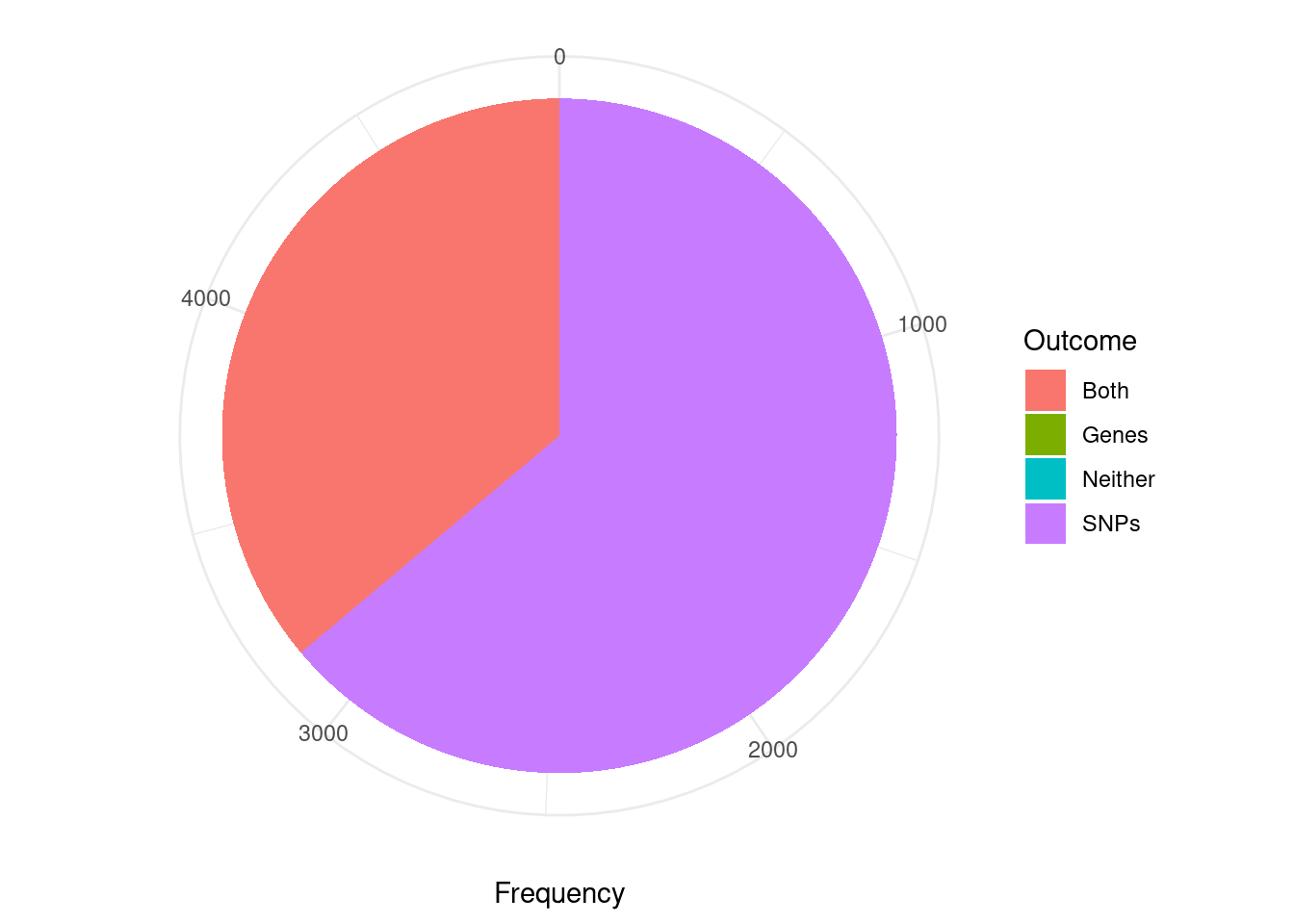
| Version | Author | Date |
|---|---|---|
| 4ded2ef | wesleycrouse | 2022-07-19 |
Analysis of TWAS False Positives by Credible Set
cTWAS is using susie settings that mask credible sets consisting of variables with minimum pairwise correlations below a specified threshold. The default threshold is 0.5. I think this is intended to mask credible sets with “diffuse” support. As a consequence, many of the genes considered here (TWAS false positives; significant z score but low PIP) are not assigned to a credible set (have cs_index=0). For this reason, the first figure is not really appropriate for answering the question “are TWAS false positives due to SNPs or genes”.
The second figure includes only TWAS genes that are assigned to a reported causal set (i.e. they are in a “pure” causal set with high pairwise correlations). I think that this figure is closer to the intended analysis. However, it may be biased in some way because we have excluded many TWAS false positive genes that are in “impure” credible sets.
Some alternatives to these figures include the region-based analysis in the previous section; or re-analysis with lower/no minimum pairwise correlation threshold (“min_abs_corr” option in susie_get_cs) for reporting credible sets.
library(ggplot2)

####################
#using only genes assigned to a credible set

pip_threshold <- 0.5

df_plot <- data.frame(Outcome=c("SNPs", "Genes", "Both", "Neither"), Frequency=rep(0,4))

for (i in 1:length(df)){
  gene_pips <- df[[i]]$gene_pips[df[[i]]$gene_pips$genename %in% df[[i]]$twas,,drop=F]
  gene_pips <- gene_pips[gene_pips$susie_pip < pip_threshold,,drop=F]

  #exclude genes that are not assigned to a credible set, cs_index==0
  gene_pips <- gene_pips[as.numeric(sapply(gene_pips$region_cs_tag, function(x){rev(unlist(strsplit(x, "_")))[1]}))!=0,]

  region_cs_pips <- df[[i]]$region_cs_pips
  rownames(region_cs_pips) <- region_cs_pips$region_cs

  gene_pips <- cbind(gene_pips, t(sapply(gene_pips$region_cs_tag, function(x){unlist(region_cs_pips[x,c("gene_pip", "snp_pip")])})))
  gene_pips$gene_pip <- gene_pips$gene_pip - gene_pips$susie_pip #subtract gene pip from causal set total to get combined pip for other genes in causal set

  plot_cutoff <- 0.5

  df_plot$Frequency[df_plot$Outcome=="Neither"] <- df_plot$Frequency[df_plot$Outcome=="Neither"] + sum(gene_pips$gene_pip < plot_cutoff & gene_pips$snp_pip < plot_cutoff)
  df_plot$Frequency[df_plot$Outcome=="Both"] <- df_plot$Frequency[df_plot$Outcome=="Both"] + sum(gene_pips$gene_pip > plot_cutoff & gene_pips$snp_pip > plot_cutoff)
  df_plot$Frequency[df_plot$Outcome=="SNPs"] <- df_plot$Frequency[df_plot$Outcome=="SNPs"] + sum(gene_pips$gene_pip < plot_cutoff & gene_pips$snp_pip > plot_cutoff)
  df_plot$Frequency[df_plot$Outcome=="Genes"] <- df_plot$Frequency[df_plot$Outcome=="Genes"] + sum(gene_pips$gene_pip > plot_cutoff & gene_pips$snp_pip < plot_cutoff)
}

pie <- ggplot(df_plot, aes(x="", y=Frequency, fill=Outcome)) + geom_bar(width = 1, stat = "identity")
pie <- pie + coord_polar("y", start=0) + theme_minimal() + theme(axis.title.y=element_blank())
pie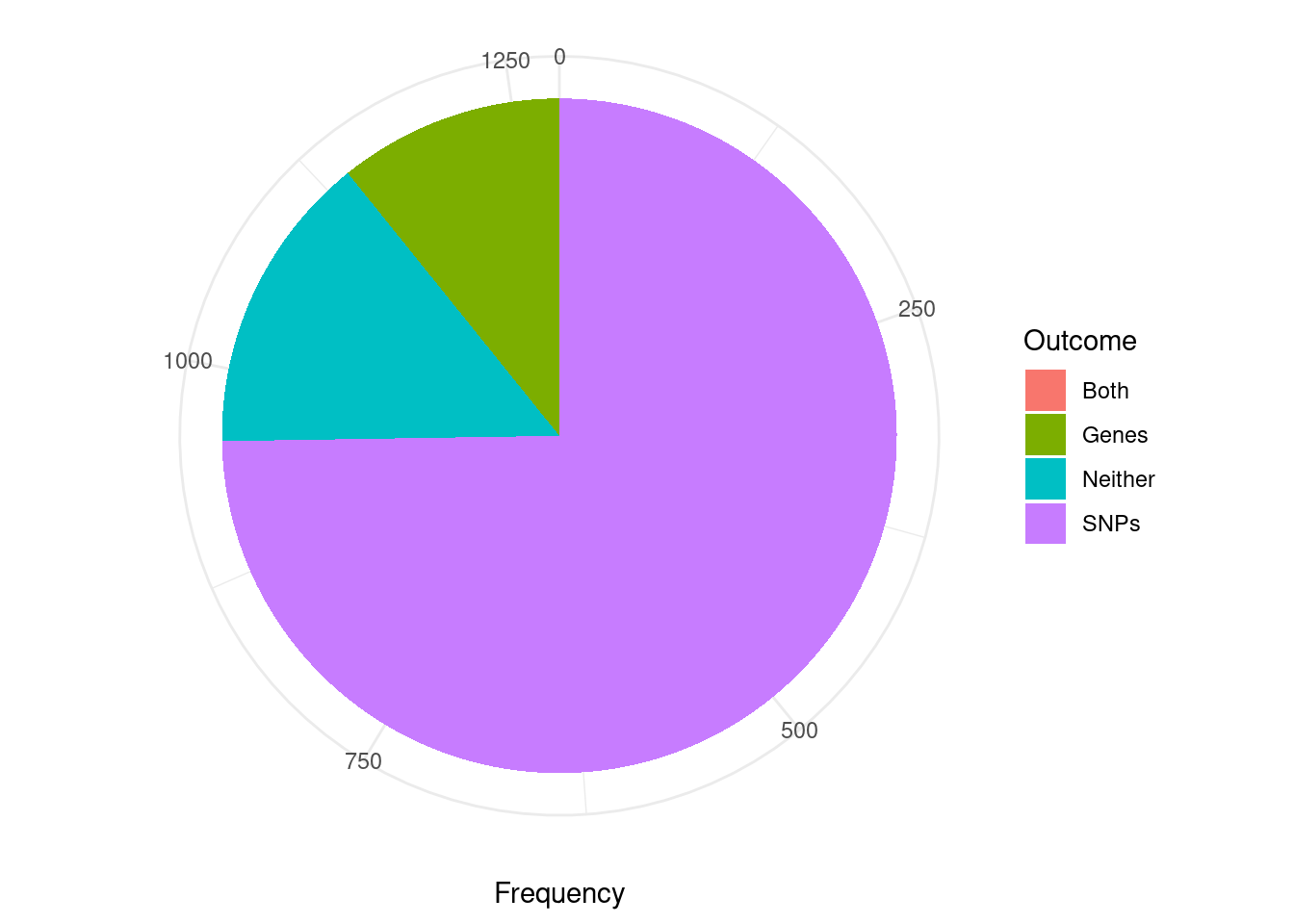
| Version | Author | Date |
|---|---|---|
| 4ded2ef | wesleycrouse | 2022-07-19 |
cTWAS genes without genome-wide significant SNP nearby
novel_genes <- data.frame(genename=as.character(), weight=as.character(), susie_pip=as.numeric(), snp_maxz=as.numeric())

for (i in 1:length(df)){
  gene_pips <- df[[i]]$gene_pips[df[[i]]$gene_pips$genename %in% df[[i]]$ctwas,,drop=F]

  region_pips <- df[[i]]$region_pips
  rownames(region_pips) <- region_pips$region

  gene_pips <- cbind(gene_pips, sapply(gene_pips$region_tag, function(x){region_pips[x,"snp_maxz"]}))
  names(gene_pips)[ncol(gene_pips)] <- "snp_maxz"

  if (nrow(gene_pips)>0){
    gene_pips$weight <- names(df)[i]
    gene_pips <- gene_pips[gene_pips$snp_maxz < qnorm(1-(5E-8/2), lower=T),c("genename", "weight", "susie_pip", "snp_maxz")]

    novel_genes <- rbind(novel_genes, gene_pips)
  }
}

novel_genes_summary <- data.frame(genename=unique(novel_genes$genename))
novel_genes_summary$nweights <- sapply(novel_genes_summary$genename, function(x){length(novel_genes$weight[novel_genes$genename==x])})
novel_genes_summary$weights <- sapply(novel_genes_summary$genename, function(x){paste(novel_genes$weight[novel_genes$genename==x],collapse=", ")})

novel_genes_summary <- novel_genes_summary[order(-novel_genes_summary$nweights),]
novel_genes_summary[,c("genename","nweights")]
genename nweights
1 PIGV 24
7 ARID1A 17
12 RINT1 13
13 ZNF467 13
8 ENPEP 9
41 MORC3 9
4 EML1 7
9 BAHCC1 7
35 GNPDA1 7
44 HSCB 7
5 ZNF415 6
49 SSBP3 6
24 LRRC10B 5
25 AATK 5
30 DNAH11 5
36 ZDHHC13 5
26 DDI2 4
27 TMEM175 4
34 PGBD2 4
37 SOX13 4
6 ASCC2 3
15 HHIPL1 3
19 GPER1 3
48 ARHGEF25 3
2 ZNF692 2
14 VDR 2
21 SLC20A2 2
33 STK38L 2
43 PUS7 2
51 SSPO 2
52 NXF1 2
62 ARL4A 2
65 GLTP 2
3 MRAS 1
10 SLC19A1 1
11 KIAA1614 1
16 CKB 1
17 REXO1 1
18 SHISA8 1
20 KIF13B 1
22 SHB 1
23 KIAA1462 1
28 SLC9A3 1
29 KHDC3L 1
31 ARMS2 1
32 PTRF 1
38 ECE2 1
39 HTRA1 1
40 SPIRE1 1
42 SCMH1 1
45 MTRF1 1
46 C22orf31 1
47 NFATC2 1
50 NUDT16L1 1
53 MAEA 1
54 TMEM179B 1
55 CPXM1 1
56 PPP3R1 1
57 CAMK1D 1
58 PYGB 1
59 NDUFAF8 1
60 NR3C1 1
61 TRIOBP 1
63 TTC33 1
64 UBASH3B 1
66 WASF3 1
67 MEX3A 1
68 KCNQ5 1
69 ATP12A 1
70 PTGER4 1
71 RABGAP1 1
72 GARNL3 1
73 MYO1F 1
74 ZKSCAN5 1
75 BIN1 1Tissue-specificity for cTWAS genes
gene_pips_by_weight <- data.frame(genename=as.character(ctwas_genes))

for (i in 1:length(df)){
  gene_pips <- df[[i]]$gene_pips
  gene_pips <- gene_pips[match(ctwas_genes, gene_pips$genename),,drop=F]

  gene_pips_by_weight <- cbind(gene_pips_by_weight, gene_pips$susie_pip)
  names(gene_pips_by_weight)[ncol(gene_pips_by_weight)] <- names(df)[i]
}

gene_pips_by_weight <- as.matrix(gene_pips_by_weight[,-1])
rownames(gene_pips_by_weight) <- ctwas_genes

#handing missing values
gene_pips_by_weight_bkup <- gene_pips_by_weight
gene_pips_by_weight[is.na(gene_pips_by_weight)] <- 0

#number of tissues with PIP>0.5 for cTWAS genes
ctwas_frequency <- rowSums(gene_pips_by_weight>0.5)

pdf(file = "output/SBP_tissue_specificity.pdf", width = 3.5, height = 2.5)

par(mar=c(4.6, 3.6, 1.1, 0.6))

hist(ctwas_frequency, col="grey", breaks=0:max(ctwas_frequency),
     #xlim=c(0,ncol(gene_pips_by_weight)),
     xlab="Number of Tissues\nwith PIP>0.5",
     ylab="Number of cTWAS Genes",
     main="SBP")

dev.off()
png
2 #heatmap of gene PIPs
cluster_ctwas_genes <- hclust(dist(gene_pips_by_weight))
cluster_ctwas_weights <- hclust(dist(t(gene_pips_by_weight)))
plot(cluster_ctwas_weights, cex=0.6)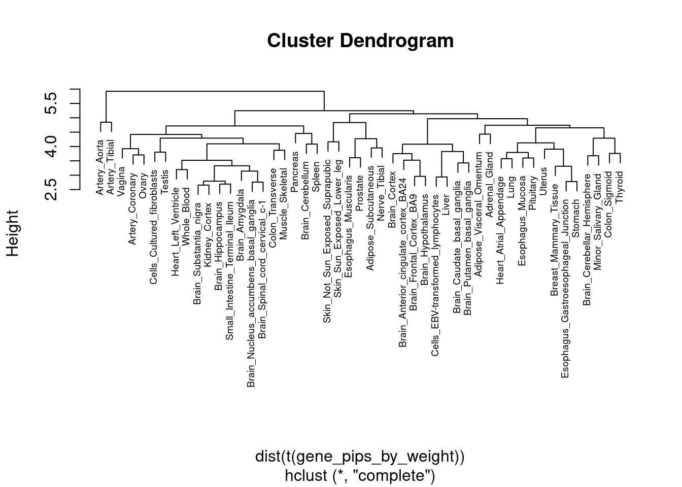
plot(cluster_ctwas_genes, cex=0.6, labels=F)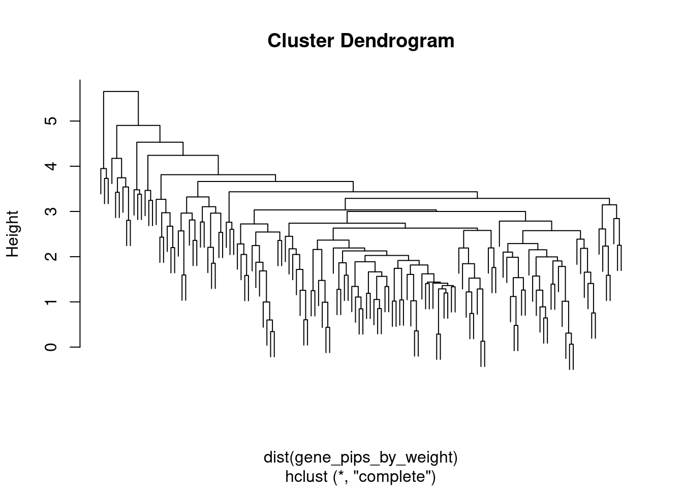
par(mar=c(14.1, 4.1, 4.1, 2.1))

image(t(gene_pips_by_weight[rev(cluster_ctwas_genes$order),rev(cluster_ctwas_weights$order)]),
      axes=F)
mtext(text=colnames(gene_pips_by_weight)[cluster_ctwas_weights$order], side=1, line=0.3, at=seq(0,1,1/(ncol(gene_pips_by_weight)-1)), las=2, cex=0.8)
mtext(text=rownames(gene_pips_by_weight)[cluster_ctwas_genes$order], side=2, line=0.3, at=seq(0,1,1/(nrow(gene_pips_by_weight)-1)), las=1, cex=0.4)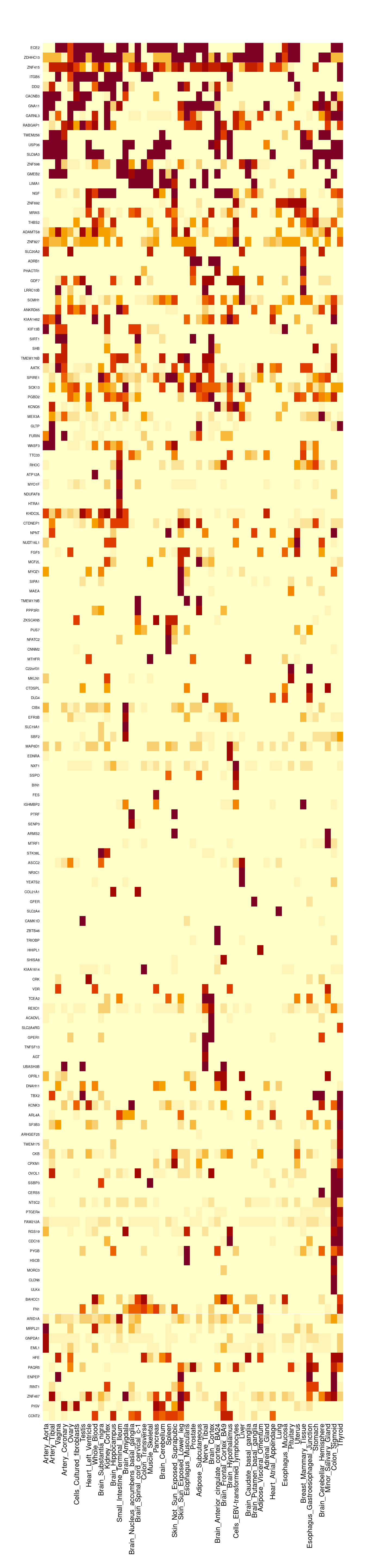
| Version | Author | Date |
|---|---|---|
| 4ded2ef | wesleycrouse | 2022-07-19 |
cTWAS genes with highest proportion of total PIP on a single tissue
#genes with highest proportion of PIP on a single tissue
gene_pips_proportion <- gene_pips_by_weight/rowSums(gene_pips_by_weight)

proportion_table <- data.frame(genename=as.character(rownames(gene_pips_proportion)))
proportion_table$max_pip_prop <- apply(gene_pips_proportion,1,max)
proportion_table$max_weight <- colnames(gene_pips_proportion)[apply(gene_pips_proportion,1,which.max)]

proportion_table[order(-proportion_table$max_pip_prop),]
genename max_pip_prop max_weight
110 FGF5 1.00000000 Kidney_Cortex
130 MEX3A 1.00000000 Skin_Sun_Exposed_Lower_leg
98 MAEA 0.99875676 Colon_Transverse
115 MKLN1 0.97998733 Muscle_Skeletal
58 GMEB2 0.86528530 Artery_Tibial
89 NFATC2 0.85197641 Brain_Putamen_basal_ganglia
131 KCNQ5 0.84570223 Skin_Sun_Exposed_Lower_leg
61 KHDC3L 0.84061553 Brain_Amygdala
56 LIMA1 0.80203430 Artery_Tibial
87 C22orf31 0.77245128 Brain_Hypothalamus
32 SHISA8 0.75316129 Adrenal_Gland
17 SBF2 0.74860882 Adipose_Visceral_Omentum
88 MCF2L 0.74584059 Brain_Nucleus_accumbens_basal_ganglia
51 NGF 0.73318270 Artery_Tibial
133 NPNT 0.69787048 Spleen
123 CIB4 0.63535143 Pancreas
93 NUDT16L1 0.58533831 Breast_Mammary_Tissue
100 SIPA1 0.57912087 Colon_Transverse
67 PTRF 0.52279594 Brain_Anterior_cingulate_cortex_BA24
129 FURIN 0.51461953 Skin_Not_Sun_Exposed_Suprapubic
39 KIF13B 0.51272444 Artery_Aorta
66 SENP3 0.50907592 Brain_Anterior_cingulate_cortex_BA24
82 PUS7 0.50000005 Brain_Cortex
118 NR3C1 0.49541239 Nerve_Tibial
22 KIAA1614 0.47037628 Adrenal_Gland
97 FES 0.46485396 Cells_Cultured_fibroblasts
83 CNNM2 0.45694930 Brain_Cortex
135 CTDNEP1 0.45235108 Spleen
42 KIAA1462 0.41231299 Artery_Aorta
77 HTRA1 0.40596140 Brain_Cerebellum
68 MYOZ1 0.39870185 Heart_Atrial_Appendage
117 YEATS2 0.38073777 Nerve_Tibial
2 ZNF692 0.37920254 Artery_Tibial
140 MYO1F 0.37638573 Uterus
141 ZKSCAN5 0.36408996 Vagina
103 PPP3R1 0.35556438 Esophagus_Mucosa
25 VDR 0.33775072 Adrenal_Gland
10 ASCC2 0.33333333 Adipose_Subcutaneous
128 WASF3 0.32735811 Skin_Not_Sun_Exposed_Suprapubic
113 CTDSPL 0.32647201 Muscle_Skeletal
111 NDUFAF8 0.31660745 Liver
35 PHACTR1 0.29949535 Artery_Aorta
142 BIN1 0.29469356 Whole_Blood
90 IGHMBP2 0.28265830 Cells_EBV-transformed_lymphocytes
69 STK38L 0.25973119 Brain_Caudate_basal_ganglia
137 MTHFR 0.25463955 Testis
134 CERS5 0.24971483 Testis
71 PGBD2 0.24580210 Brain_Cerebellum
65 ARMS2 0.24538598 Brain_Anterior_cingulate_cortex_BA24
50 DDI2 0.24355662 Artery_Tibial
28 CRK 0.23865670 Adrenal_Gland
127 GLTP 0.23860434 Skin_Sun_Exposed_Lower_leg
119 COL21A1 0.23527011 Nerve_Tibial
40 SLC20A2 0.22270011 Artery_Tibial
34 GDF7 0.22216643 Artery_Aorta
86 MTRF1 0.21760060 Brain_Hypothalamus
36 THBS2 0.21657342 Artery_Tibial
105 GFER 0.21256922 Esophagus_Muscularis
121 ARL4A 0.21001323 Skin_Not_Sun_Exposed_Suprapubic
104 NT5C2 0.20454015 Esophagus_Muscularis
99 TMEM179B 0.20421809 Colon_Transverse
94 SSPO 0.19861458 Vagina
81 SCMH1 0.19740514 Brain_Cortex
107 CAMK1D 0.19692855 Heart_Left_Ventricle
95 NXF1 0.19484101 Skin_Sun_Exposed_Lower_leg
55 ADRB1 0.19382029 Artery_Tibial
74 SLC2A4RG 0.18824677 Colon_Sigmoid
21 SLC19A1 0.18689736 Adipose_Visceral_Omentum
116 DLG4 0.18675657 Muscle_Skeletal
37 GPER1 0.18130484 Esophagus_Muscularis
101 OVOL1 0.18021505 Colon_Transverse
132 ATP12A 0.16942324 Skin_Sun_Exposed_Lower_leg
124 RHOC 0.16867997 Skin_Sun_Exposed_Lower_leg
14 MAP6D1 0.16844930 Adipose_Visceral_Omentum
52 ITGB5 0.16426940 Artery_Tibial
43 SIRT1 0.16144703 Artery_Aorta
139 GARNL3 0.15776539 Thyroid
79 SPIRE1 0.15748760 Brain_Cerebellum
59 ZBTB46 0.15741013 Brain_Anterior_cingulate_cortex_BA24
70 SF3B3 0.15661207 Brain_Caudate_basal_ganglia
138 RABGAP1 0.15589825 Thyroid
75 SOX13 0.15474869 Brain_Cerebellum
16 EDNRA 0.15322874 Adipose_Visceral_Omentum
45 AATK 0.15284475 Artery_Aorta
41 SHB 0.15197641 Artery_Aorta
5 MRAS 0.15001252 Adipose_Subcutaneous
62 TMEM256 0.14604304 Brain_Amygdala
112 AGT 0.14603708 Muscle_Skeletal
18 ADAMTS8 0.14221312 Artery_Aorta
44 LRRC10B 0.13846628 Artery_Tibial
31 TCEA2 0.13757005 Adrenal_Gland
91 ARHGEF25 0.13605510 Thyroid
33 ANKRD65 0.13562392 Artery_Aorta
122 EFR3B 0.13473451 Pancreas
30 REXO1 0.13453839 Adrenal_Gland
125 TTC33 0.13436213 Skin_Not_Sun_Exposed_Suprapubic
54 ZNF827 0.13090289 Artery_Tibial
84 ACADVL 0.12594934 Colon_Sigmoid
49 TNFSF13 0.12551020 Artery_Coronary
136 PTGER4 0.12340344 Stomach
108 SLC2A4 0.12077665 Heart_Left_Ventricle
85 HSCB 0.11193490 Heart_Left_Ventricle
46 GNA11 0.11069596 Artery_Aorta
78 ZNF598 0.10947675 Brain_Cerebellum
38 TMEM176B 0.10932998 Artery_Aorta
73 ZDHHC13 0.10909762 Brain_Hypothalamus
60 SLC9A3 0.10204381 Brain_Amygdala
96 CACNB3 0.10048107 Prostate
47 MRPL21 0.09573165 Brain_Frontal_Cortex_BA9
29 USP36 0.09393167 Adrenal_Gland
53 TMEM175 0.09277207 Pancreas
106 CDC16 0.09246813 Muscle_Skeletal
26 HHIPL1 0.09067948 Adrenal_Gland
27 CKB 0.09039347 Adrenal_Gland
63 CLCN6 0.08781225 Skin_Sun_Exposed_Lower_leg
3 KCNK3 0.08745834 Adipose_Subcutaneous
120 TRIOBP 0.08700981 Nerve_Tibial
76 ECE2 0.08588711 Brain_Cerebellum
15 ENPEP 0.08140599 Adipose_Visceral_Omentum
92 SSBP3 0.07579230 Skin_Sun_Exposed_Lower_leg
19 BAHCC1 0.07447531 Ovary
48 PAQR5 0.07401120 Artery_Tibial
126 UBASH3B 0.07387624 Skin_Not_Sun_Exposed_Suprapubic
23 RINT1 0.07304682 Cells_EBV-transformed_lymphocytes
102 CPXM1 0.07267484 Colon_Transverse
109 PYGB 0.07166966 Heart_Left_Ventricle
57 TBX2 0.07124038 Minor_Salivary_Gland
8 ZNF415 0.07041728 Adipose_Visceral_Omentum
114 FAM212A 0.06841141 Muscle_Skeletal
9 RGS19 0.06818204 Breast_Mammary_Tissue
80 MORC3 0.06685889 Brain_Cerebellum
64 DNAH11 0.06483962 Brain_Cortex
7 EML1 0.06425825 Adipose_Subcutaneous
72 GNPDA1 0.06344780 Spleen
13 ULK4 0.06281785 Artery_Tibial
20 OPRL1 0.05874841 Prostate
11 ARID1A 0.05760531 Cells_Cultured_fibroblasts
12 FN1 0.05351843 Artery_Aorta
6 HFE 0.05178007 Small_Intestine_Terminal_Ileum
4 CCNT2 0.03637705 Adipose_Subcutaneous
24 ZNF467 0.03634890 Artery_Aorta
1 PIGV 0.03298222 Brain_Caudate_basal_gangliaGenes nearby and nearest to GWAS peaks
#####load positions for all genes on autosomes in ENSEMBL, subset to only protein coding and lncRNA with non-missing HGNC symbol
library(biomaRt)

# ensembl <- useEnsembl(biomart="ENSEMBL_MART_ENSEMBL", dataset="hsapiens_gene_ensembl")
# G_list <- getBM(filters= "chromosome_name", attributes= c("hgnc_symbol","chromosome_name","start_position","end_position","gene_biotype", "ensembl_gene_id", "strand"), values=1:22, mart=ensembl)
#
# save(G_list, file=paste0("G_list_", trait_id, ".RData"))
load(paste0("G_list_", trait_id, ".RData"))

G_list <- G_list[G_list$gene_biotype %in% c("protein_coding"),]
G_list$hgnc_symbol[G_list$hgnc_symbol==""] <- "-"
G_list$tss <- G_list[,c("end_position", "start_position")][cbind(1:nrow(G_list),G_list$strand/2+1.5)]

#####load z scores from the analysis and add positions from the LD reference
# results_dir <- results_dirs[1]
# weight <- rev(unlist(strsplit(results_dir, "/")))[1]
# weight <- unlist(strsplit(weight, split="_nolnc"))
# analysis_id <- paste(trait_id, weight, sep="_")
#
# load(paste0(results_dir, "/", analysis_id, "_expr_z_snp.Rd"))
#
# LDR_dir <- "/project2/mstephens/wcrouse/UKB_LDR_0.1/"
# LDR_files <- list.files(LDR_dir)
# LDR_files <- LDR_files[grep(".Rvar" ,LDR_files)]
#
# z_snp$chrom <- as.integer(NA)
# z_snp$pos <- as.integer(NA)
#
# for (i in 1:length(LDR_files)){
#   print(i)
#
#   LDR_info <- read.table(paste0(LDR_dir, LDR_files[i]), header=T)
#   z_snp_index <- which(z_snp$id %in% LDR_info$id)
#   z_snp[z_snp_index,c("chrom", "pos")] <- t(sapply(z_snp_index, function(x){unlist(LDR_info[match(z_snp$id[x], LDR_info$id),c("chrom", "pos")])}))
# }
#
# z_snp <- z_snp[,c("id", "z", "chrom","pos")]
# save(z_snp, file=paste0("z_snp_pos_", trait_id, ".RData"))
load(paste0("z_snp_pos_", trait_id, ".RData"))

####################
#identify genes within 500kb of genome-wide significant variant ("nearby")
G_list$nearby <- NA

window_size <- 500000

for (chr in 1:22){
  #index genes on chromosome
  G_list_index <- which(G_list$chromosome_name==chr)

  #subset z_snp to chromosome, then subset to significant genome-wide significant variants
  z_snp_chr <- z_snp[z_snp$chrom==chr,,drop=F]
  z_snp_chr <- z_snp_chr[abs(z_snp_chr$z)>qnorm(1-(5E-8/2), lower=T),,drop=F]

  #iterate over genes on chromsome and check if a genome-wide significant SNP is within the window
  for (i in G_list_index){
    window_start <- G_list$start_position[i] - window_size
    window_end <- G_list$end_position[i] + window_size
    G_list$nearby[i] <- any(z_snp_chr$pos>=window_start & z_snp_chr$pos<=window_end)
  }
}

####################
#identify genes that are nearest to lead genome-wide significant variant ("nearest")
G_list$nearest <- F
G_list$distance <- Inf
G_list$which_nearest <- NA

window_size <- 500000

n_peaks <- 0

for (chr in 1:22){
  #index genes on chromosome
  G_list_index <- which(G_list$chromosome_name==chr & G_list$gene_biotype=="protein_coding")

  #subset z_snp to chromosome, then subset to significant genome-wide significant variants
  z_snp_chr <- z_snp[z_snp$chrom==chr,,drop=F]
  z_snp_chr <- z_snp_chr[abs(z_snp_chr$z)>qnorm(1-(5E-8/2), lower=T),,drop=F]

  while (nrow(z_snp_chr)>0){
    n_peaks <- n_peaks + 1

    lead_index <- which.max(abs(z_snp_chr$z))
    lead_position <- z_snp_chr$pos[lead_index]

    distances <- sapply(G_list_index, function(i){
      if (lead_position >= G_list$start_position[i] & lead_position <= G_list$end_position[i]){
        distance <- 0
      } else {
        distance <- min(abs(G_list$start_position[i] - lead_position), abs(G_list$end_position[i] - lead_position))
      }
      distance
    })

    min_distance <- min(distances)

    G_list$nearest[G_list_index[distances==min_distance]] <- T

    nearest_genes <- paste0(G_list$hgnc_symbol[G_list_index[distances==min_distance]], collapse=", ")

    update_index <- which(G_list$distance[G_list_index] > distances)
    G_list$distance[G_list_index][update_index] <- distances[update_index]
    G_list$which_nearest[G_list_index][update_index] <- nearest_genes

    window_start <- lead_position - window_size
    window_end <- lead_position + window_size
    z_snp_chr <- z_snp_chr[!(z_snp_chr$pos>=window_start & z_snp_chr$pos<=window_end),,drop=F]
  }
}

G_list$distance[G_list$distance==Inf] <- NA

#report number of GWAS peaks
sum(n_peaks)
[1] 217Enrichment analysis using known silver standard genes
known_genes <- read.table("data/Giri_2018_SBP.txt", header=F)
known_genes <- as.character(unique(known_genes[,1]))

dbs <- c("GO_Biological_Process_2021")
GO_enrichment <- enrichr(known_genes, dbs)
Uploading data to Enrichr... Done.
Querying GO_Biological_Process_2021... Done.
Parsing results... Done.for (db in dbs){
cat(paste0(db, "\n\n"))
enrich_results <- GO_enrichment[[db]]
enrich_results <- enrich_results[enrich_results$Adjusted.P.value<0.05,c("Term", "Overlap", "Adjusted.P.value", "Genes")]
print(enrich_results)
print(plotEnrich(GO_enrichment[[db]]))
}GO_Biological_Process_2021
[1] Term Overlap Adjusted.P.value Genes
<0 rows> (or 0-length row.names)
save(enrich_results, file="output/Giri_SBP_genes_enrichment.RData")
write.csv(enrich_results, file="output/Giri_SBP_genes_enrichment.csv")

enrich_results <- read.table("output/Giri_SBP_genes_enrichment.csv", header=T, sep=",")

#report number of known IBD genes in annotations
length(known_genes)
[1] 53Summary table for selected tissue groups
#mapping genename to ensembl
genename_mapping <- data.frame(genename=as.character(), ensembl_id=as.character(), weight=as.character())

for (i in 1:length(results_dirs)){
  results_dir <- results_dirs[i]
  weight <- rev(unlist(strsplit(results_dir, "/")))[1]
  analysis_id <- paste(trait_id, weight, sep="_")

  sqlite <- RSQLite::dbDriver("SQLite")
  db = RSQLite::dbConnect(sqlite, paste0("/project2/mstephens/wcrouse/predictdb_nolnc/mashr_", weight, ".db"))
  query <- function(...) RSQLite::dbGetQuery(db, ...)
  gene_info <- query("select gene, genename, gene_type from extra")
  RSQLite::dbDisconnect(db)

  genename_mapping <- rbind(genename_mapping, cbind(gene_info[,c("gene","genename")],weight))
}

genename_mapping <- genename_mapping[,c("gene","genename"),drop=F]
genename_mapping <- genename_mapping[!duplicated(genename_mapping),]
selected_groups <- c("Cardiovascular")
selected_genes <- unique(unlist(sapply(df_group[selected_groups], function(x){x$ctwas})))
weight_groups <- weight_groups[order(weight_groups$group),]
selected_weights <- weight_groups$weight[weight_groups$group %in% selected_groups]
gene_pips_by_weight <- gene_pips_by_weight_bkup
results_table <- as.data.frame(round(gene_pips_by_weight[selected_genes,selected_weights],3))
results_table$n_discovered <- apply(results_table>0.8,1,sum,na.rm=T)
results_table$n_imputed <- apply(results_table, 1, function(x){sum(!is.na(x))-1})
results_table$ensembl_gene_id <- genename_mapping$gene[sapply(rownames(results_table), match, table=genename_mapping$genename)]
results_table$ensembl_gene_id <- sapply(results_table$ensembl_gene_id, function(x){unlist(strsplit(x, "[.]"))[1]})
results_table <- cbind(results_table, G_list[sapply(results_table$ensembl_gene_id, match, table=G_list$ensembl_gene_id),c("chromosome_name","start_position","end_position","nearby","nearest","distance","which_nearest")])
results_table$known <- rownames(results_table) %in% known_genes
load(paste0("group_enrichment_results_", trait_id, ".RData"))
group_enrichment_results$group <- as.character(group_enrichment_results$group)
group_enrichment_results$db <- as.character(group_enrichment_results$db)
group_enrichment_results <- group_enrichment_results[group_enrichment_results$group %in% selected_groups,,drop=F]
results_table$enriched_terms <- sapply(rownames(results_table), function(x){paste(group_enrichment_results$Term[grep(x, group_enrichment_results$Genes)],collapse="; ")})
write.csv(results_table, file=paste0("summary_table_SBP_nolnc_corrected.csv"))Results and figures for the paper
Gene expression explains a small proportion of heritability
These MESC results use matching summary statistics and GTEx v8 models provided by MESC.
library(ggrepel)

mesc_results <- as.data.frame(data.table::fread("output/allweight_heritability.txt"))
mesc_results <- mesc_results[mesc_results$trait==trait_id,]
mesc_results$`h2med/h2g` <- mesc_results$h2med/mesc_results$h2
mesc_results$weight[!is.na(mesc_results$weight_predictdb)] <- mesc_results$weight_predictdb[!is.na(mesc_results$weight_predictdb)]
mesc_results <- mesc_results[,colnames(mesc_results)!="weight_predictdb"]
rownames(mesc_results) <- mesc_results$weight

output$pve_med <- output$pve_g / (output$pve_g + output$pve_s)
rownames(output) <- output$weight

df_plot <- output
df_plot <- df_plot[mesc_results$weight,]
df_plot$mesc <- as.numeric(mesc_results$`h2med/h2g`)
df_plot$ctwas <- as.numeric(df_plot$pve_med)
df_plot$tissue <- as.character(sapply(df_plot$weight, function(x){paste(unlist(strsplit(x, "_")), collapse=" ")}))

df_plot$label <- ""
label_list <- c("Artery Aorta", "Artery Tibial")

df_plot$label[df_plot$tissue %in% label_list] <- df_plot$tissue[df_plot$tissue %in% label_list]

####################

pdf(file = "output/SBP_cTWAS_vs_MESC.pdf", width = 4, height = 3)

p <- ggplot(df_plot, aes(mesc, ctwas, label = label)) + geom_point(color = "blue", size=1.5)
p <- p + geom_text_repel(size=3,
                         max.time=20,
                         max.iter=400000,
                         seed=1,
                         max.overlaps=Inf,
                         #force=2.8,
                         #force_pull=0.3,
                         force=1,
                         force_pull=1,
                         min.segment.length=0)
p <- p + ylab("(Gene PVE) / (Total PVE) using cTWAS") + xlab("(h2med) / (h2g) using MESC")
p <- p + geom_abline(slope=1, intercept=0, linetype=3, alpha=0.4)

xy_min <- min(df_plot$mesc, df_plot$ctwas, na.rm=T)
xy_max <- max(df_plot$mesc, df_plot$ctwas, na.rm=T)

p <- p + xlim(xy_min,xy_max) + ylim(xy_min,xy_max)

fit <- lm(ctwas~0+mesc, data=df_plot)
p <- p + geom_abline(slope=summary(fit)$coefficients["mesc","Estimate"], intercept=0, linetype=2, color="blue", alpha=0.4)

p <- p + theme_bw()


p <- p + theme(axis.title = element_text(color = "grey20", size = 10)) + ggtitle("SBP")

p
Warning: Removed 1 rows containing missing values (geom_point).Warning: Removed 1 rows containing missing values (geom_text_repel).dev.off()png
2 pWarning: Removed 1 rows containing missing values (geom_point).
Warning: Removed 1 rows containing missing values (geom_text_repel).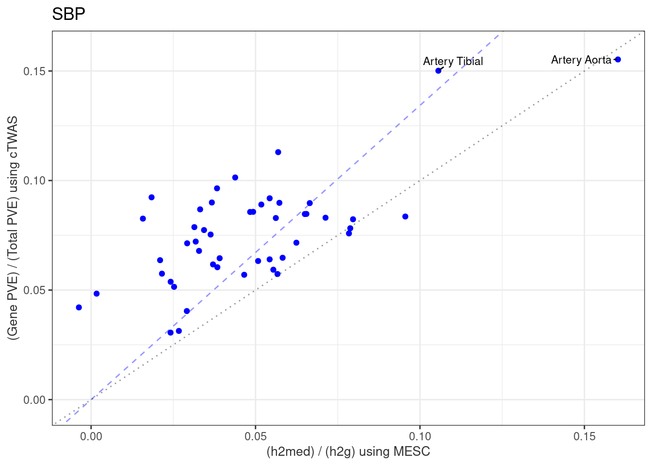
| Version | Author | Date |
|---|---|---|
| 2af4567 | wesleycrouse | 2022-09-02 |
| 0b519f1 | wesleycrouse | 2022-07-28 |
| c19144f | wesleycrouse | 2022-07-28 |
| 0f5b69a | wesleycrouse | 2022-07-28 |
| cb3f976 | wesleycrouse | 2022-07-27 |
| dd9f346 | wesleycrouse | 2022-07-27 |
| ea9958c | wesleycrouse | 2022-07-25 |
| 3be2b06 | wesleycrouse | 2022-07-25 |
| d34b3a0 | wesleycrouse | 2022-07-19 |
####################

df_plot$tissue_number <- order(df_plot$weight)

df_plot$legend_entry <- sapply(1:nrow(df_plot), function(x){paste0(df_plot$tissue_number[x], ": ", df_plot$tissue[x])})


png(filename = "output/SBP_cTWAS_vs_MESC_v2.png", width = 6, height = 5, units = "in", res=150)

p <- ggplot(df_plot, aes(mesc, ctwas, label = tissue_number))

p <- p + geom_point(color = "blue", size=1.5)

p <- p + geom_text_repel(min.segment.length=0,
                         size=2.4,
                         seed=1,
                         max.overlaps=Inf,
                         force=2,
                         force_pull=0.5)
p <- p + ylab("(Gene PVE) / (Total PVE) using cTWAS") + xlab("(h2med) / (h2g) using MESC")

p <- p + geom_abline(slope=1, intercept=0, linetype=3, alpha=0.4)

xy_min <- min(df_plot$mesc, df_plot$ctwas, na.rm=T)
xy_max <- max(df_plot$mesc, df_plot$ctwas, na.rm=T)

p <- p + xlim(xy_min,xy_max) + ylim(xy_min,xy_max)

fit <- lm(ctwas~0+mesc, data=df_plot)
p <- p + geom_abline(slope=summary(fit)$coefficients["mesc","Estimate"], intercept=0, linetype=2, color="blue", alpha=0.4)

p <- p + theme_bw()

#p <- p + theme(plot.margin = unit(c(1,15,1,1), "lines"))
# y_values <- xy_max-(xy_max-xy_min)*(1:nrow(df_plot))/nrow(df_plot)
# p <- p + geom_text(aes(label=legend_entry, x=xy_max, y=y_values, hjust=0))

p
Warning: Removed 1 rows containing missing values (geom_point).
Warning: Removed 1 rows containing missing values (geom_text_repel).dev.off()png
2 pWarning: Removed 1 rows containing missing values (geom_point).
Warning: Removed 1 rows containing missing values (geom_text_repel).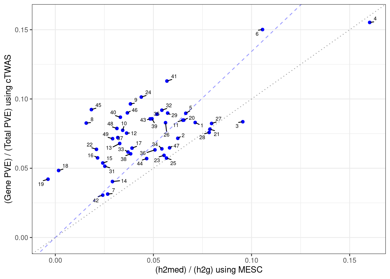
| Version | Author | Date |
|---|---|---|
| eb3c5bf | wesleycrouse | 2022-09-27 |
| 3349d12 | wesleycrouse | 2022-09-16 |
| 6a57156 | wesleycrouse | 2022-09-14 |
| 220ba1d | wesleycrouse | 2022-09-09 |
| 2af4567 | wesleycrouse | 2022-09-02 |
| 0b519f1 | wesleycrouse | 2022-07-28 |
| c19144f | wesleycrouse | 2022-07-28 |
| 0f5b69a | wesleycrouse | 2022-07-28 |
| cb3f976 | wesleycrouse | 2022-07-27 |
| dd9f346 | wesleycrouse | 2022-07-27 |
| ea9958c | wesleycrouse | 2022-07-25 |
| 3be2b06 | wesleycrouse | 2022-07-25 |
| d34b3a0 | wesleycrouse | 2022-07-19 |
####################

#report correlation between cTWAS and MESC
cor(df_plot$mesc, df_plot$ctwas, use="complete.obs")
[1] 0.6896666cTWAS finds fewer genes than TWAS
library(ggrepel)

df_plot <- output
#df_plot <- df_plot[selected_weights,,drop=F]
df_plot$tissue <- sapply(df_plot$weight, function(x){paste(unlist(strsplit(x,"_")),collapse=" ")})

png(filename = "output/SBP_cTWAS_vs_TWAS_all.png", width = 6, height = 5, units = "in", res=150)

p <- ggplot(df_plot, aes(n_twas, n_ctwas, label = tissue))
p <- p + geom_point(color = "blue", size=1.5)
p <- p + geom_text_repel(min.segment.length=0,
                         size=2.4,
                         seed=1,
                         max.overlaps=Inf,
                         force=2,
                         force_pull=0.5)
p <- p + ylab("Number of cTWAS genes") + xlab("Number of TWAS genes")
p <- p + scale_y_continuous(breaks=seq(0,max(df_plot$n_ctwas),2))
p <- p + scale_x_continuous(breaks=seq(0,max(df_plot$n_twas),5))
p <- p + theme_bw()

fit <- lm(n_ctwas~0+n_twas, data=df_plot)
p <- p + geom_abline(slope=summary(fit)$coefficients["n_twas","Estimate"], intercept=0, linetype=2, color="blue")

p

dev.off()
png
2 #report correlation between cTWAS and TWAS
cor(df_plot$n_ctwas, df_plot$n_twas)[1] 0.6818165####################
#using cutpoint for number of ctwas and twas genes to determine which tissues to label
df_plot <- output
df_plot$tissue <- sapply(df_plot$weight, function(x){paste(unlist(strsplit(x,"_")),collapse=" ")})
df_plot$tissue[df_plot$n_ctwas < 11.5 & df_plot$n_twas < 135] <- ""
png(filename = "output/SBP_cTWAS_vs_TWAS_top.png", width = 6, height = 5, units = "in", res=150)
p <- ggplot(df_plot, aes(n_twas, n_ctwas, label = tissue))
p <- p + geom_point(color = "blue", size=1.5)
p <- p + geom_text_repel(min.segment.length=0,
size=2.4,
seed=1,
max.overlaps=Inf,
force=1,
force_pull=0.5)
p <- p + ylab("Number of cTWAS genes") + xlab("Number of TWAS genes")
p <- p + scale_y_continuous(breaks=seq(0,max(df_plot$n_ctwas),2))
p <- p + scale_x_continuous(breaks=seq(0,max(df_plot$n_twas),5))
p <- p + theme_bw()
fit <- lm(n_ctwas~0+n_twas, data=df_plot)
p <- p + geom_abline(slope=summary(fit)$coefficients["n_twas","Estimate"], intercept=0, linetype=2, color="blue")
p
dev.off()png
2 p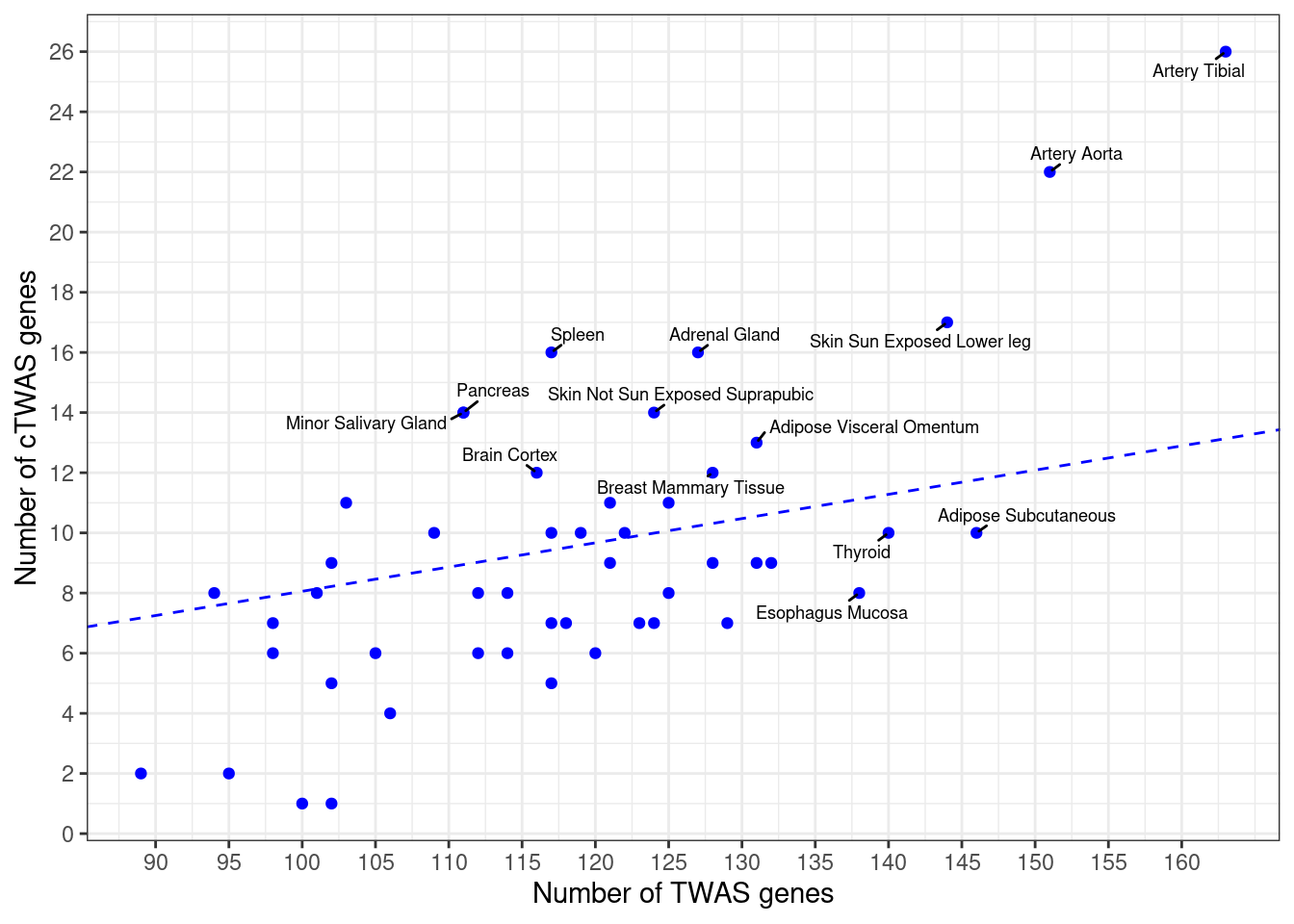
####################
#only labeling genes in selected tissue groups

df_plot <- output
df_plot$tissue <- sapply(df_plot$weight, function(x){paste(unlist(strsplit(x,"_")),collapse=" ")})

df_plot[!(df_plot$weight %in% selected_weights),"tissue"] <- ""

png(filename = "output/SBP_cTWAS_vs_TWAS_selected.png", width = 6, height = 5, units = "in", res=150)

p <- ggplot(df_plot, aes(n_twas, n_ctwas, label = tissue))
p <- p + geom_point(color = "blue", size=1.5)
p <- p + geom_text_repel(min.segment.length=0,
                         size=2.4,
                         seed=1,
                         max.overlaps=Inf,
                         force=1,
                         force_pull=0.5)
p <- p + ylab("Number of cTWAS genes") + xlab("Number of TWAS genes")
p <- p + scale_y_continuous(breaks=seq(0,max(df_plot$n_ctwas),2))
p <- p + scale_x_continuous(breaks=seq(0,max(df_plot$n_twas),5))
p <- p + theme_bw()

fit <- lm(n_ctwas~0+n_twas, data=df_plot)
p <- p + geom_abline(slope=summary(fit)$coefficients["n_twas","Estimate"], intercept=0, linetype=2, color="blue")

p

dev.off()
png
2 p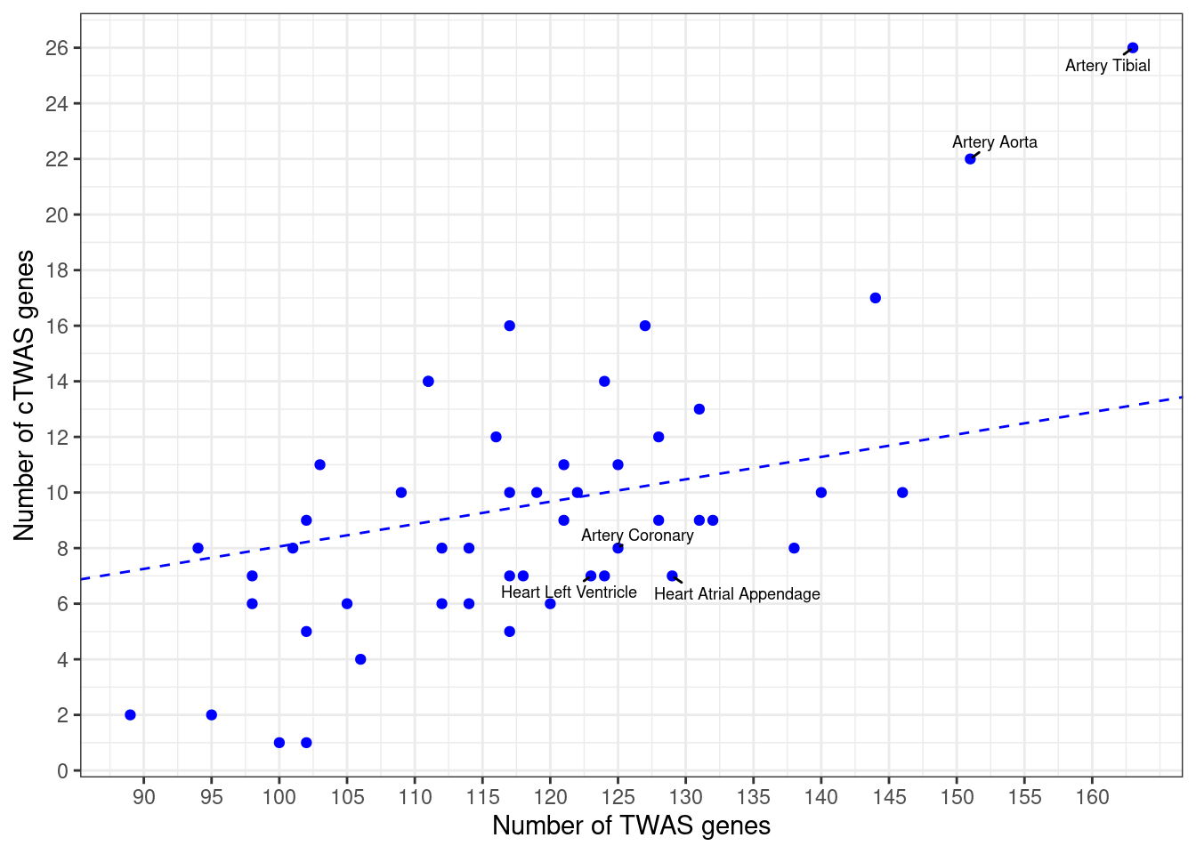
####################
#minimum and maximum number of discoveries per tissues
min(output$n_ctwas)
[1] 1max(output$n_ctwas)[1] 26min(output$n_twas)[1] 89max(output$n_twas)[1] 163####################
df_plot <- output
df_plot$tissue <- sapply(df_plot$weight, function(x){paste(unlist(strsplit(x,"_")),collapse=" ")})
df_plot$label <- ""
#label_list <- c("Artery Aorta", "Artery Tibial")
label_list <- c(df_plot$tissue[which.max(df_plot$n_twas)], df_plot$tissue[which.max(df_plot$n_ctwas)])
df_plot$label[df_plot$tissue %in% label_list] <- df_plot$tissue[df_plot$tissue %in% label_list]
pdf(file = "output/SBP_cTWAS_vs_TWAS.pdf", width = 4, height = 3)
p <- ggplot(df_plot, aes(n_twas, n_ctwas, label = label))
p <- p + geom_point(color = "blue", size=1.5)
p <- p + geom_text_repel(min.segment.length=0,
size=3,
seed=1,
max.overlaps=Inf,
force=1,
force_pull=1)
p <- p + ylab("Number of cTWAS Genes") + xlab("Number of TWAS Genes")
p <- p + scale_y_continuous(breaks=seq(0,max(df_plot$n_ctwas),2))
p <- p + scale_x_continuous(breaks=seq(0,max(df_plot$n_twas),10))
p <- p + theme_bw()
fit <- lm(n_ctwas~0+n_twas, data=df_plot)
p <- p + geom_abline(slope=summary(fit)$coefficients["n_twas","Estimate"], intercept=0, linetype=2, color="blue", alpha=0.4) + ggtitle("SBP")
p
dev.off()png
2 Most cTWAS genes were found in a small number of tissues
#number of tissues with PIP>0.5 for cTWAS genes
gene_pips_by_weight_bkup <- gene_pips_by_weight
gene_pips_by_weight[is.na(gene_pips_by_weight)] <- 0

gene_pips_by_weight <- gene_pips_by_weight[apply(gene_pips_by_weight[,selected_weights,drop=F],1,max)>0.8,,drop=F]

ctwas_frequency <- rowSums(gene_pips_by_weight>0.5)
hist(ctwas_frequency, col="grey", breaks=0:max(ctwas_frequency), xlim=c(0,max(ctwas_frequency)),
     xlab="Number of Tissues with PIP>0.5",
     ylab="Number of cTWAS Genes",
     main="")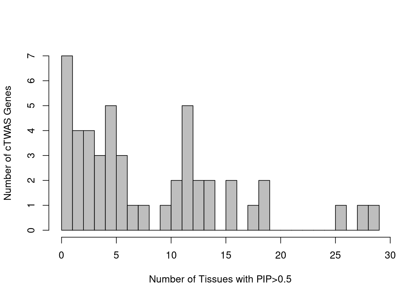
#report number of genes in each tissue bin
table(ctwas_frequency)
ctwas_frequency
1 2 3 4 5 6 7 8 10 11 12 13 14 16 18 19 26 28 29
7 4 4 3 5 3 1 1 1 2 5 2 2 2 1 2 1 1 1 #% less than 5
sum(ctwas_frequency<5)/length(ctwas_frequency)[1] 0.375#% equal to 1
sum(ctwas_frequency==1)/length(ctwas_frequency)[1] 0.1458333#list the frequency for each gene
ctwas_frequency PIGV ZNF692 KCNK3 CCNT2 HFE EML1 ZNF415 ARID1A FN1 ULK4 ENPEP ADAMTS8 RINT1 ZNF467 ANKRD65 GDF7 PHACTR1 THBS2 GPER1 TMEM176B KIF13B SLC20A2 SHB KIAA1462 SIRT1 LRRC10B AATK GNA11 MRPL21 PAQR5 TNFSF13 DDI2 NGF ITGB5 TMEM175 ZNF827 ADRB1 LIMA1 TBX2 GMEB2 ZBTB46 MYOZ1 MORC3 HSCB CDC16 CAMK1D SLC2A4 PYGB
26 2 12 28 19 16 12 18 19 16 12 5 14 29 4 4 3 3 3 6 1 2 5 1 1 5 6 10 11 12 3 4 1 5 13 2 1 1 14 1 7 2 13 8 11 5 6 12 Many cTWAS genes are novel - selected tissues
“Novel” is defined as 1) not in the silver standard, and 2) not the gene nearest to a genome-wide significant GWAS peak
save.image("SBP_workspace.RData")

#barplot of number of cTWAS genes in each tissue
df_plot <- output[output$weight %in% selected_weights,,drop=F]
df_plot <- df_plot[order(-df_plot$n_ctwas),,drop=F]

df_plot$tissue <- sapply(df_plot$weight, function(x){paste(unlist(strsplit(x,"_")),collapse=" ")})

pdf(file = "output/SBP_novel_ctwas_genes.pdf", width = 2.75, height = 3)

par(mar=c(6.6, 3.6, 1.1, 0.6))

barplot(df_plot$n_ctwas, names.arg=df_plot$tissue, las=2, ylab="Number of cTWAS Genes", main="",
        cex.lab=0.7,
        cex.axis=0.7,
        cex.names=0.6,
        axis.lty=1)


results_table$novel <- !(results_table$nearest | results_table$known)
df_plot$n_novel <- sapply(df_plot$weight, function(x){sum(results_table[df[[x]]$ctwas,"novel"], na.rm=T)})

barplot(df_plot$n_novel, names.arg=df_plot$tissue, las=2, col="blue", add=T, xaxt='n', yaxt='n')

legend("topright",
       legend = c("Silver Standard or\nNearest to GWAS Peak", "Novel"),
       fill = c("grey", "blue"), cex=0.6)

dev.off()
png
2 Number of cTWAS Genes - all tissues
df_plot <- output
df_plot <- df_plot[order(df_plot$n_ctwas),,drop=F]

df_plot$tissue <- sapply(df_plot$weight, function(x){paste(unlist(strsplit(x,"_")),collapse=" ")})

pdf(file = "output/SBP_number_ctwas_genes.pdf", width = 7, height = 5)

par(mar=c(3.6, 8.6, 0.6, 1.6))

barplot(df_plot$n_ctwas, names.arg=df_plot$tissue, las=2, xlab="Number of cTWAS Genes", main="",
        cex.lab=0.8,
        cex.axis=0.8,
        cex.names=0.5,
        axis.lty=1,
        col=c("darkblue", "grey50"),
        horiz=T,
        las=1)

grid(nx = NULL,
     ny = NA,
     lty = 2, col = "grey", lwd = 1)

dev.off()
png
2 Summary table of results
selected_weights_whitespace <- sapply(selected_weights, function(x){paste(unlist(strsplit(x, "_")), collapse=" ")})

results_summary <- data.frame(genename=as.character(rownames(results_table)),
                              ensembl_gene_id=results_table$ensembl_gene_id,
                              gene_biotype=G_list$gene_biotype[sapply(results_table$ensembl_gene_id, match, table=G_list$ensembl_gene_id)],
                              chromosome=results_table$chromosome_name,
                              start_position=results_table$start_position,
                              max_pip_tissue=selected_weights_whitespace[apply(results_table[,selected_weights], 1, which.max)],
                              max_pip=apply(results_table[,selected_weights], 1, max, na.rm=T),
                              other_tissues_detected=apply(results_table[,selected_weights],1,function(x){paste(selected_weights_whitespace[which(x>0.8 & x!=max(x,na.rm=T))], collapse="; ")}),
                              nearby=results_table$nearby,
                              nearest=results_table$nearest,
                              distance=G_list$distance[sapply(results_table$ensembl_gene_id, match, table=G_list$ensembl_gene_id)],
                              known=results_table$known,
                              enriched_terms=results_table$enriched_terms)

results_summary <- results_summary[order(results_summary$chromosome, results_summary$start_position),]

write.csv(results_summary, file=paste0("results_summary_SBP_nolnc_corrected.csv"))
GO enrichment for genes in selected tissues
#enrichment for cTWAS genes using enrichR
library(enrichR)

dbs <- c("GO_Biological_Process_2021")

GO_enrichment <- enrichr(selected_genes, dbs)
Uploading data to Enrichr... Warning in enrichr(selected_genes, dbs): genes must be a non-empty vector of gene names or a data.frame with genes and score.Done.
Querying GO_Biological_Process_2021... Done.
Parsing results... Done.for (db in dbs){
cat(paste0(db, "\n\n"))
enrich_results <- GO_enrichment[[db]]
enrich_results <- enrich_results[enrich_results$Adjusted.P.value<0.05,c("Term", "Overlap", "Adjusted.P.value", "Genes"),drop=F]
print(enrich_results)
print(plotEnrich(GO_enrichment[[db]]))
}GO_Biological_Process_2021
[1] Term Overlap Adjusted.P.value Genes
<0 rows> (or 0-length row.names)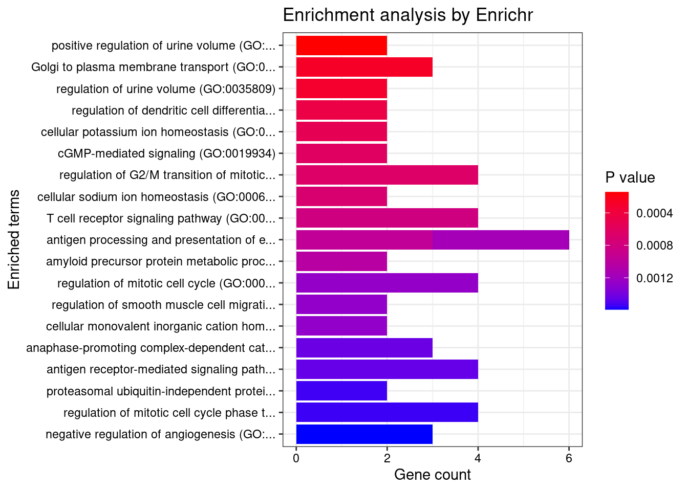
| Version | Author | Date |
|---|---|---|
| 220ba1d | wesleycrouse | 2022-09-09 |
Summary table of results - version 2
results_summary <- data.frame(genename=as.character(rownames(results_table)),
                              ensembl_gene_id=results_table$ensembl_gene_id,
                              chromosome=results_table$chromosome_name,
                              start_position=results_table$start_position,
                              max_pip_tissue=selected_weights_whitespace[apply(results_table[,selected_weights], 1, which.max)],
                              max_pip_tissue_nospace=selected_weights[apply(results_table[,selected_weights], 1, which.max)],
                              max_pip=apply(results_table[,selected_weights], 1, max, na.rm=T),
                              other_tissues_detected=apply(results_table[,selected_weights],1,function(x){paste(selected_weights_whitespace[which(x>0.8 & x!=max(x,na.rm=T))], collapse="; ")}),
                              region_tag_tissue=NA,
                              z_tissue=NA,
                              num_eqtl_tissue=NA,
                              twas_fp_tissue=NA,
                              gene_nearest_region_peak_tissue=NA,
                              nearby=results_table$nearby,
                              nearest=results_table$nearest,
                              distance=results_table$distance,
                              which_nearest=results_table$which_nearest,
                              known=results_table$known,
                              stringsAsFactors=F)

for (i in 1:nrow(results_summary)){
  tissue <- results_summary$max_pip_tissue_nospace[i]
  gene <- results_summary$genename[i]
  gene_pips <- df[[tissue]]$gene_pips
  results_summary[i,c("region_tag_tissue", "z_tissue", "num_eqtl_tissue")] <- gene_pips[gene_pips$genename==gene,c("region_tag", "z", "num_eqtl")]
  region_tag <- results_summary$region_tag_tissue[i]
  results_summary$twas_fp_tissue[i] <- any(gene_pips$genename[gene_pips$region_tag==region_tag & gene_pips$genename!=gene] %in% df[[tissue]]$twas)


  region_pips <- df[[tissue]]$region_pips
  lead_snp <- region_pips$which_snp_maxz[region_pips$region==region_tag]

  chromosome <- results_summary$chromosome[i]
  lead_position <- z_snp$pos[z_snp$id==lead_snp]

  G_list_index <- which(G_list$chromosome_name==chromosome)

  distances <- sapply(G_list_index, function(i){
    if (lead_position >= G_list$start_position[i] & lead_position <= G_list$end_position[i]){
      distance <- 0
    } else {
      distance <- min(abs(G_list$start_position[i] - lead_position), abs(G_list$end_position[i] - lead_position))
    }
    distance
  })

  results_summary$gene_nearest_region_peak_tissue[i] <- paste0(G_list$hgnc_symbol[G_list_index[which(distances==min(distances))]], collapse="; ")

}

####################
#GO enrichment of cTWAS genes
# genes <- results_summary$genename
#
# dbs <- c("GO_Biological_Process_2021", "GO_Cellular_Component_2021", "GO_Molecular_Function_2021")
# GO_enrichment <- enrichr(genes, dbs)
#
# save(GO_enrichment, file=paste0(trait_id, "_enrichment_results.RData"))

####################
#enrichment of silver standard genes
# genes <- known_genes
#
# dbs <- c("GO_Biological_Process_2021", "GO_Cellular_Component_2021", "GO_Molecular_Function_2021")
# GO_enrichment_silver_standard <- enrichr(genes, dbs)
#
# save(GO_enrichment_silver_standard, file=paste0(trait_id, "_silver_standard_enrichment_results.RData"))

####################
#report GO cTWAS

load(paste0(trait_id, "_enrichment_results.RData"))

GO_enrichment <- do.call(rbind, GO_enrichment)
GO_enrichment$db <- sapply(rownames(GO_enrichment), function(x){unlist(strsplit(x, split="[.]"))[1]})
rownames(GO_enrichment) <- NULL

GO_enrichment <- GO_enrichment[GO_enrichment$Adjusted.P.value < 0.05,]
GO_enrichment <- GO_enrichment[order(-GO_enrichment$Odds.Ratio),]

results_summary$GO <- sapply(results_summary$genename, function(x){terms <- GO_enrichment$Term[grep(x, GO_enrichment$Genes)];
                                             if (length(terms)>0){terms <- terms[1:min(length(terms),5)]};
                                             paste0(terms, collapse="; ")})


####################
#report GO silver standard

GO_silver_standard_sigthresh <- 0.1

load(paste0(trait_id, "_silver_standard_enrichment_results.RData"))

GO_enrichment_silver_standard <- do.call(rbind, GO_enrichment_silver_standard)
GO_enrichment_silver_standard$db <- sapply(rownames(GO_enrichment_silver_standard), function(x){unlist(strsplit(x, split="[.]"))[1]})
rownames(GO_enrichment_silver_standard) <- NULL

GO_enrichment_silver_standard <- GO_enrichment_silver_standard[order(GO_enrichment_silver_standard$Adjusted.P.value),]
write.csv(GO_enrichment_silver_standard, file=paste0("output/SBP_silver_standard_enrichment_results.csv"))

GO_enrichment_silver_standard <- GO_enrichment_silver_standard[GO_enrichment_silver_standard$Adjusted.P.value < GO_silver_standard_sigthresh,]
GO_enrichment_silver_standard <- GO_enrichment_silver_standard[order(-GO_enrichment_silver_standard$Odds.Ratio),]

#reload GO cTWAS for GO crosswalk
load(paste0(trait_id, "_enrichment_results.RData"))

GO_enrichment <- do.call(rbind, GO_enrichment)
GO_enrichment$db <- sapply(rownames(GO_enrichment), function(x){unlist(strsplit(x, split="[.]"))[1]})
rownames(GO_enrichment) <- NULL

#overlap between sets
GO_enrichment <- GO_enrichment[GO_enrichment$Term %in% GO_enrichment_silver_standard$Term,,drop=F]
GO_enrichment_silver_standard <- GO_enrichment_silver_standard[GO_enrichment_silver_standard$Term %in% GO_enrichment$Term,,drop=F]
GO_enrichment <- GO_enrichment[match(GO_enrichment_silver_standard$Term, GO_enrichment$Term),]

results_summary$GO_silver <- sapply(results_summary$genename, function(x){terms <- GO_enrichment$Term[grep(x, GO_enrichment$Genes)];
                                                                          if (length(terms)>0){terms <- terms[1:min(length(terms),5)]};
                                                                          paste0(terms, collapse="; ")})

####################
#report FUMA

FUMA <- data.table::fread(paste0("/project2/xinhe/shengqian/cTWAS/cTWAS_analysis/data/FUMA_output/", trait_id, "/GS.txt"))
FUMA <- FUMA[FUMA$Category %in% c("GO_bp", "GO_cc", "GO_mf"),,drop=F]
FUMA <- FUMA[order(FUMA$p),]

write.csv(FUMA, file="output/SBP_MAGMA.csv")

#reload GO cTWAS for GO crosswalk
load(paste0(trait_id, "_enrichment_results.RData"))
GO_enrichment <- do.call(rbind, GO_enrichment)
GO_enrichment$db <- sapply(rownames(GO_enrichment), function(x){unlist(strsplit(x, split="[.]"))[1]})
rownames(GO_enrichment) <- NULL

GO_enrichment$Term_FUMA <- sapply(GO_enrichment$Term, function(x){rev(rev(unlist(strsplit(x, split=" [(]GO")))[-1])})
GO_enrichment$Term_FUMA <- paste0("GO_", toupper(gsub(" ", "_", GO_enrichment$Term_FUMA)))

#overlap between sets
GO_enrichment <- GO_enrichment[GO_enrichment$Term_FUMA %in% FUMA$GeneSet,,drop=F]
FUMA <- FUMA[FUMA$GeneSet %in% GO_enrichment$Term_FUMA]
GO_enrichment <- GO_enrichment[match(FUMA$GeneSet, GO_enrichment$Term_FUMA),]

results_summary$GO_MAGMA <- sapply(results_summary$genename, function(x){terms <- GO_enrichment$Term[grep(x, GO_enrichment$Genes)];
                                                                         if (length(terms)>0){terms <- terms[1:min(length(terms),5)]};
                                                                         paste0(terms, collapse="; ")})

####################
#report FUMA + susieGO

# gsesusie <- as.data.frame(readxl::read_xlsx("gsesusie_enrichment.xlsx", sheet=trait_id))
# gsesusie$GeneSet <- paste0("(", gsesusie$GeneSet, ")")
#
# #reload GO cTWAS for GO crosswalk
# load(paste0(trait_id, "_enrichment_results.RData"))
# GO_enrichment <- do.call(rbind, GO_enrichment)
# GO_enrichment$db <- sapply(rownames(GO_enrichment), function(x){unlist(strsplit(x, split="[.]"))[1]})
# rownames(GO_enrichment) <- NULL
#
# GO_enrichment$GeneSet <- sapply(GO_enrichment$Term, function(x){rev(unlist(strsplit(x, " ")))[1]})
#
# #overlap between sets
# GO_enrichment <- GO_enrichment[GO_enrichment$GeneSet %in% gsesusie$GeneSet,,drop=F]
# gsesusie <- gsesusie[gsesusie$GeneSet %in% GO_enrichment$GeneSet,,drop=F]
# GO_enrichment <- GO_enrichment[match(gsesusie$GeneSet, GO_enrichment$GeneSet),]
#
# results_summary$GO_MAGMA_SuSiE <- sapply(results_summary$genename, function(x){terms <- GO_enrichment$Term[grep(x, GO_enrichment$Genes)];
#                                                                          if (length(terms)>0){terms <- terms[1:min(length(terms),5)]};
#                                                                          paste0(terms, collapse="; ")})

####################

results_summary <- results_summary[order(results_summary$chromosome, results_summary$start_position),]
results_summary <- results_summary[,!(colnames(results_summary) %in% c("max_pip_tissue_nospace"))]

write.csv(results_summary, file=paste0("results_summary_SBP_nolnc_v2_corrected.csv"))

#number of genes in silver standard or at least one enriched term from GO silver standard
sum(results_summary$GO_silver!="" | results_summary$known)
[1] 20#number of genes in silver standard or at least one enriched term from GO silver standard or GO MAGMA
sum(results_summary$GO_silver!="" | results_summary$GO_MAGMA!="" | results_summary$known)[1] 20#number of genes in silver standard or at least one enriched term from GO silver standard or GO MAGMA or GO cTWAS
#sum(results_summary$GO_silver!="" | results_summary$GO_MAGMA!="" | results_summary$known | results_summary$GO!="")Summary table of results - Compact version
results_summary_compact <- results_summary[results_summary$max_pip>0.9,]

results_summary_compact$evidence  <- ""
results_summary_compact$evidence[which(results_summary_compact$known==T & results_summary_compact$nearest==T)] <- "S,G"
results_summary_compact$evidence[which(results_summary_compact$known==T & results_summary_compact$nearest!=T)] <- "S"
results_summary_compact$evidence[which(results_summary_compact$known!=T & results_summary_compact$nearest==T)] <- "G"

results_summary_compact <- results_summary_compact[,c("genename", "max_pip_tissue", "max_pip", "other_tissues_detected", "evidence")]

write.csv(results_summary_compact, file=paste0("results_summary_SBP_compact.csv"), row.names=F)
Novel Genes by Tissue Group
#barplot of number of cTWAS genes in each tissue
df_plot <- -sort(-sapply(groups[groups!="None"], function(x){length(df_group[[x]][["ctwas"]])}))

par(mar=c(10.1, 4.1, 4.1, 2.1))
barplot(df_plot, las=2, ylab="Number of cTWAS Genes", main="")

df_plot_novel <- rep(NA, length(df_plot))
names(df_plot_novel) <- names(df_plot)

for (i in 1:length(df_plot)){
  genename <- df_group[[names(df_plot)[i]]]$ctwas
  gene <- genename_mapping$gene[match(genename, genename_mapping$genename)]
  gene <- sapply(gene, function(x){unlist(strsplit(x, "[.]"))[1]})

  G_list_subset <- G_list[match(gene, G_list$ensembl_gene_id),]

  G_list_subset$known <- G_list_subset$hgnc_symbol %in% known_genes

  df_plot_novel[i] <- sum(!(G_list_subset$known | G_list_subset$nearest), na.rm=T)
}

barplot(df_plot_novel, las=2, col="blue", add=T, xaxt='n', yaxt='n')

legend("topright",
       legend = c("Silver Standard or\nNearest to GWAS Peak", "Novel"),
       fill = c("grey", "blue"))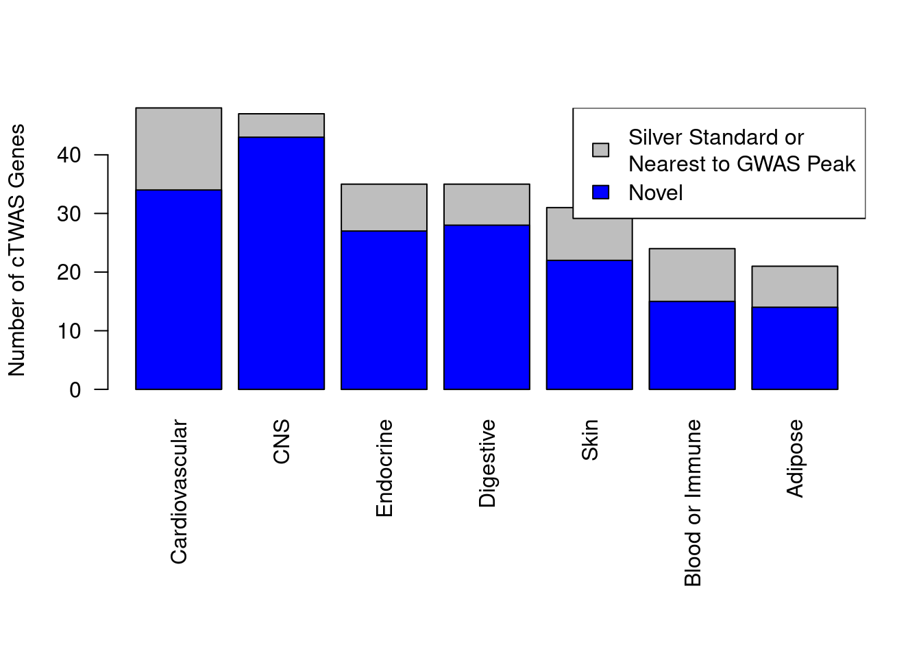
| Version | Author | Date |
|---|---|---|
| 220ba1d | wesleycrouse | 2022-09-09 |
##########

#barplot of number of cTWAS genes in each tissue
df_plot <- -sort(-sapply(groups[groups!="None"], function(x){length(df_group[[x]][["ctwas"]])}))

df_plot_novel <- rep(NA, length(df_plot))
names(df_plot_novel) <- names(df_plot)

for (i in 1:length(df_plot)){
  genename <- df_group[[names(df_plot)[i]]]$ctwas
  gene <- genename_mapping$gene[match(genename, genename_mapping$genename)]
  gene <- sapply(gene, function(x){unlist(strsplit(x, "[.]"))[1]})

  G_list_subset <- G_list[match(gene, G_list$ensembl_gene_id),]

  G_list_subset$known <- G_list_subset$hgnc_symbol %in% known_genes

  df_plot_novel[i] <- sum(!(G_list_subset$known | G_list_subset$nearest), na.rm=T)
}

pdf(file = "output/SBP_novel_ctwas_genes_group.pdf", width = 2.75, height = 3)
par(mar=c(4.6, 3.6, 1.1, 0.6))

barplot(df_plot, las=2, col="blue", ylab="Number of cTWAS Genes", main="",
        cex.lab=0.8,
        cex.axis=0.8,
        cex.names=0.7,
        axis.lty=1)
barplot(df_plot-df_plot_novel, las=2, add=T, xaxt='n', yaxt='n')

legend("topright",
       legend = c("Silver Standard or\nNearest to GWAS Peak", "Novel"),
       fill = c("grey", "blue"), cex=0.5)

dev.off()
png
2 Updated locus plots
load(paste0("G_list_", trait_id, ".RData"))
G_list <- G_list[G_list$gene_biotype %in% c("protein_coding"),]
G_list$hgnc_symbol[G_list$hgnc_symbol==""] <- "-"
G_list$tss <- G_list[,c("end_position", "start_position")][cbind(1:nrow(G_list),G_list$strand/2+1.5)]

####################

locus_plot_final <- function(genename=NULL, tissue=NULL, xlim=NULL, return_table=F, label_panel="TWAS", label_genes=NULL, label_pos=NULL, plot_eqtl=NULL, draw_gene_track=T, legend_side="right"){
  results_dir <- results_dirs[grep(tissue, results_dirs)]
  weight <- rev(unlist(strsplit(results_dir, "/")))[1]
  weight <- unlist(strsplit(weight, split="_nolnc"))
  analysis_id <- paste(trait_id, weight, sep="_")

  #load ctwas results
  ctwas_res <- data.table::fread(paste0(results_dir, "/", analysis_id, "_ctwas.susieIrss.txt"))

  #make unique identifier for regions and effects
  ctwas_res$region_tag <- paste(ctwas_res$region_tag1, ctwas_res$region_tag2, sep="_")
  ctwas_res$region_cs_tag <- paste(ctwas_res$region_tag, ctwas_res$cs_index, sep="_")

  #load z scores for SNPs
  load(paste0(results_dir, "/", analysis_id, "_expr_z_snp.Rd"))

  #separate gene and SNP results
  ctwas_gene_res <- ctwas_res[ctwas_res$type == "gene", ]
  ctwas_gene_res <- data.frame(ctwas_gene_res)
  ctwas_snp_res <- ctwas_res[ctwas_res$type == "SNP", ]
  ctwas_snp_res <- data.frame(ctwas_snp_res)

  #add gene information to results
  sqlite <- RSQLite::dbDriver("SQLite")
  db = RSQLite::dbConnect(sqlite, paste0("/project2/mstephens/wcrouse/predictdb_nolnc/mashr_", weight, "_nolnc.db"))
  query <- function(...) RSQLite::dbGetQuery(db, ...)
  gene_info <- query("select gene, genename, gene_type from extra")
  RSQLite::dbDisconnect(db)

  ctwas_gene_res <- cbind(ctwas_gene_res, gene_info[sapply(ctwas_gene_res$id, match, gene_info$gene), c("genename", "gene_type")])

  #add z scores to results
  load(paste0(results_dir, "/", analysis_id, "_expr_z_gene.Rd"))
  ctwas_gene_res$z <- z_gene[ctwas_gene_res$id,]$z

  z_snp <- z_snp[z_snp$id %in% ctwas_snp_res$id,]
  ctwas_snp_res$z <- z_snp$z[match(ctwas_snp_res$id, z_snp$id)]

  #merge gene and snp results with added information
  ctwas_snp_res$genename=NA
  ctwas_snp_res$gene_type=NA

  ctwas_res <- rbind(ctwas_gene_res, ctwas_snp_res[,colnames(ctwas_gene_res)])

  region_tag <- ctwas_res$region_tag[which(ctwas_res$genename==genename)]

  region_tag1 <- unlist(strsplit(region_tag, "_"))[1]
  region_tag2 <- unlist(strsplit(region_tag, "_"))[2]

  a <- ctwas_res[ctwas_res$region_tag==region_tag,]

  rm(ctwas_res)

  regionlist <- readRDS(paste0(results_dir, "/", analysis_id, "_ctwas.regionlist.RDS"))
  region <- regionlist[[as.numeric(region_tag1)]][[region_tag2]]

  R_snp_info <- do.call(rbind, lapply(region$regRDS, function(x){data.table::fread(paste0(tools::file_path_sans_ext(x), ".Rvar"))}))

  a_pos_bkup <- a$pos
  a$pos[a$type=="gene"] <- G_list$tss[match(sapply(a$id[a$type=="gene"], function(x){unlist(strsplit(x, "[.]"))[1]}) ,G_list$ensembl_gene_id)]
  a$pos[is.na(a$pos)] <- a_pos_bkup[is.na(a$pos)]
  a$pos <- a$pos/1000000

  if (!is.null(xlim)){

    if (is.na(xlim[1])){
      xlim[1] <- min(a$pos)
    }

    if (is.na(xlim[2])){
      xlim[2] <- max(a$pos)
    }

    a <- a[a$pos>=xlim[1] & a$pos<=xlim[2],,drop=F]
  }

  focus <- genename

  if (is.null(label_genes)){
    label_genes <- focus
  }

  if (is.null(label_pos)){
    label_pos <- rep(3, length(label_genes))
  }

  if (is.null(plot_eqtl)){
    plot_eqtl <- focus
  }

  focus <- a$id[which(a$genename==focus)]
  a$focus <- 0
  a$focus <- as.numeric(a$id==focus)

  a$PVALUE <- (-log(2) - pnorm(abs(a$z), lower.tail=F, log.p=T))/log(10)

  R_gene <- readRDS(region$R_g_file)
  R_snp_gene <- readRDS(region$R_sg_file)
  R_snp <- as.matrix(Matrix::bdiag(lapply(region$regRDS, readRDS)))

  rownames(R_gene) <- region$gid
  colnames(R_gene) <- region$gid
  rownames(R_snp_gene) <- R_snp_info$id
  colnames(R_snp_gene) <- region$gid
  rownames(R_snp) <- R_snp_info$id
  colnames(R_snp) <- R_snp_info$id

  a$r2max <- NA
  a$r2max[a$type=="gene"] <- R_gene[focus,a$id[a$type=="gene"]]
  a$r2max[a$type=="SNP"] <- R_snp_gene[a$id[a$type=="SNP"],focus]

  r2cut <- 0.4
  colorsall <- c("#7fc97f", "#beaed4", "#fdc086")

  start <- min(a$pos)
  end <- max(a$pos)

  if (draw_gene_track){
    layout(matrix(1:4, ncol = 1), widths = 1, heights = c(1.5,0.25,1.5,0.75), respect = FALSE)
  } else {
    layout(matrix(1:3, ncol = 1), widths = 1, heights = c(1.5,0.25,1.5), respect = FALSE)
  }

  par(mar = c(0, 4.1, 0, 2.1))

  plot(a$pos[a$type=="SNP"], a$PVALUE[a$type == "SNP"], pch = 21, xlab=paste0("Chromosome ", region_tag1, " position (Mb)"), frame.plot=FALSE, bg = colorsall[1], ylab = "-log10(p value)", panel.first = grid(), ylim =c(0, max(a$PVALUE)*1.1), xaxt = 'n', xlim=c(start, end))

  points(a$pos[a$type=="SNP" & a$r2max > r2cut], a$PVALUE[a$type == "SNP"  & a$r2max > r2cut], pch = 21, bg = "purple")
  points(a$pos[a$type=="SNP" & a$focus == 1], a$PVALUE[a$type == "SNP" & a$focus == 1], pch = 21, bg = "salmon")
  points(a$pos[a$type=="gene"], a$PVALUE[a$type == "gene"], pch = 22, bg = colorsall[1], cex = 2)
  points(a$pos[a$type=="gene" & a$r2max > r2cut], a$PVALUE[a$type == "gene"  & a$r2max > r2cut], pch = 22, bg = "purple", cex = 2)
  points(a$pos[a$type=="gene" & a$focus == 1], a$PVALUE[a$type == "gene" & a$focus == 1], pch = 22, bg = "salmon", cex = 2)

  alpha=0.05
  abline(h=-log10(alpha/nrow(ctwas_gene_res)), col ="red", lty = 2)

  if (label_panel=="TWAS"){
    for (i in 1:length(label_genes)){
      text(a$pos[a$genename==label_genes[i]], a$PVALUE[a$genename==label_genes[i]], labels=label_genes[i], pos=label_pos[i], cex=0.7)
    }
  }

  par(mar = c(0.25, 4.1, 0.25, 2.1))

  plot(NA, xlim = c(start, end), ylim = c(0, length(plot_eqtl)), frame.plot = F, axes = F, xlab = NA, ylab = NA)

  for (i in 1:length(plot_eqtl)){
    cgene <- a$id[which(a$genename==plot_eqtl[i])]
    load(paste0(results_dir, "/",analysis_id, "_expr_chr", region_tag1, ".exprqc.Rd"))
    eqtls <- rownames(wgtlist[[cgene]])
    eqtl_pos <- a$pos[a$id %in% eqtls]

    col="grey"

    rect(start, length(plot_eqtl)+1-i-0.8, end, length(plot_eqtl)+1-i-0.2, col = col, border = T, lwd = 1)

    if (length(eqtl_pos)>0){
      for (j in 1:length(eqtl_pos)){
        segments(x0=eqtl_pos[j], x1=eqtl_pos[j], y0=length(plot_eqtl)+1-i-0.2, length(plot_eqtl)+1-i-0.8, lwd=1.5)
      }
    }
  }

  text(start, length(plot_eqtl)-(1:length(plot_eqtl))+0.5,
       labels = plot_eqtl, srt = 0, pos = 2, xpd = TRUE, cex=0.7)

  par(mar = c(4.1, 4.1, 0, 2.1))

  plot(a$pos[a$type=="SNP"], a$PVALUE[a$type == "SNP"], pch = 19, xlab=paste0("Chromosome ", region_tag1, " position (Mb)"),frame.plot=FALSE, col = "white", ylim= c(0,1.1), ylab = "cTWAS PIP", xlim = c(start, end))

  grid()
  points(a$pos[a$type=="SNP"], a$susie_pip[a$type == "SNP"], pch = 21, xlab="Genomic position", bg = colorsall[1])
  points(a$pos[a$type=="SNP" & a$r2max > r2cut], a$susie_pip[a$type == "SNP"  & a$r2max >r2cut], pch = 21, bg = "purple")
  points(a$pos[a$type=="SNP" & a$focus == 1], a$susie_pip[a$type == "SNP" & a$focus == 1], pch = 21, bg = "salmon")
  points(a$pos[a$type=="gene"], a$susie_pip[a$type == "gene"], pch = 22, bg = colorsall[1], cex = 2)
  points(a$pos[a$type=="gene" & a$r2max > r2cut], a$susie_pip[a$type == "gene"  & a$r2max > r2cut], pch = 22, bg = "purple", cex = 2)
  points(a$pos[a$type=="gene" & a$focus == 1], a$susie_pip[a$type == "gene" & a$focus == 1], pch = 22, bg = "salmon", cex = 2)

  x_pos <- ifelse(legend_side=="right", max(a$pos)-0.2*(max(a$pos)-min(a$pos)), min(a$pos)+0.05*(max(a$pos)-min(a$pos)))

  legend(x_pos, y= 1 ,c("Gene", "SNP","Lead TWAS Gene", "R2 > 0.4", "R2 <= 0.4"), pch = c(22,21,19,19,19), col = c("black", "black", "salmon", "purple", colorsall[1]), cex=0.7, title.adj = 0)

  if (label_panel=="cTWAS"){
    for (i in 1:length(label_genes)){
      text(a$pos[a$genename==label_genes[i]], a$susie_pip[a$genename==label_genes[i]], labels=label_genes[i], pos=label_pos[i], cex=0.7)
    }
  }

  if (draw_gene_track){
    source("code/trackplot.R")

    query_ucsc = TRUE
    build = "hg38"
    col = "gray70"
    txname = NULL
    genename = NULL
    collapse_txs = TRUE
    gene_model = "data/hg38.ensGene.gtf.gz"
    isGTF = T

    ##########
    start <- min(a$pos)*1000000
    end <- max(a$pos)*1000000
    chr <- paste0("chr",as.character(unique(a$chrom)))

    #collect gene models
    if(is.null(gene_model)){
      if(query_ucsc){
        message("Missing gene model. Trying to query UCSC genome browser..")
        etbl = .extract_geneModel_ucsc(chr, start = start, end = end, refBuild = build, txname = txname, genename = genename)
      } else{
        etbl = NULL
      }
    } else{
      if(isGTF){
        etbl = .parse_gtf(gtf = gene_model, chr = chr, start = start, end = end, txname = txname, genename = genename)
      } else{
        etbl = .extract_geneModel(ucsc_tbl = gene_model, chr = chr, start = start, end = end, txname = txname, genename = genename)
      }
    }

    #draw gene models
    if(!is.null(etbl)){
      if(collapse_txs){
        etbl = .collapse_tx(etbl)
      }

      #subset to protein coding genes in ensembl and lincRNAs included in the analysis
      #etbl <- etbl[names(etbl) %in% G_list$ensembl_gene_id]
      etbl <- etbl[names(etbl) %in% c(G_list$ensembl_gene_id[G_list$gene_biotype=="protein_coding"], sapply(a$id[a$type=="gene"], function(x){unlist(strsplit(x, split="[.]"))[1]}))]

      for (i in 1:length(etbl)){
        ensembl_name <- attr(etbl[[i]], "gene")
        gene_name <- G_list$hgnc_symbol[match(ensembl_name, G_list$ensembl_gene_id)]
        if (gene_name=="" | is.na(gene_name)){
          gene_name <- a$genename[sapply(a$id, function(x){unlist(strsplit(x,split="[.]"))[1]})==ensembl_name]
        }
        if (length(gene_name)>0){
          attr(etbl[[i]], "gene") <- gene_name
        }

        attr(etbl[[i]], "imputed") <- ensembl_name %in% sapply(ctwas_gene_res$id, function(x){unlist(strsplit(x, split="[.]"))[1]})

      }

      par(mar = c(0, 4.1, 0, 2.1))

      plot(NA, xlim = c(start, end), ylim = c(0, length(etbl)), frame.plot = FALSE, axes = FALSE, xlab = NA, ylab = NA)

      etbl <- etbl[order(-sapply(etbl, function(x){attr(x, "start")}))]

      for(tx_id in 1:length(etbl)){
        txtbl = etbl[[tx_id]]

        if (attr(txtbl, "imputed")){
          exon_col = "#192a56"
        } else {
          exon_col = "darkred"
        }

        segments(x0 = attr(txtbl, "start"), y0 = tx_id-0.45, x1 = attr(txtbl, "end"), y1 = tx_id-0.45, col = exon_col, lwd = 1)

        if(is.na(attr(txtbl, "tx"))){
          text(x = start, y = tx_id-0.45, labels = paste0(attr(txtbl, "gene")), cex = 0.7, adj = 0, srt = 0, pos = 2, xpd = TRUE)
        } else {
          text(x = start, y = tx_id-0.45, labels = paste0(attr(txtbl, "tx"), " [", attr(txtbl, "gene"), "]"), cex = 0.7, adj = 0, srt = 0, pos = 2, xpd = TRUE)
        }

        rect(xleft = txtbl[[1]], ybottom = tx_id-0.75, xright = txtbl[[2]], ytop = tx_id-0.25, col = exon_col, border = NA)
        if(attr(txtbl, "strand") == "+"){
          dirat = pretty(x = c(min(txtbl[[1]]), max(txtbl[[2]])))
          dirat[1] = min(txtbl[[1]]) #Avoid drawing arrows outside gene length
          dirat[length(dirat)] = max(txtbl[[2]])
          points(x = dirat, y = rep(tx_id-0.45, length(dirat)), pch = ">", col = exon_col)
        }else{
          dirat = pretty(x = c(min(txtbl[[1]]), max(txtbl[[2]])))
          dirat[1] = min(txtbl[[1]]) #Avoid drawing arrows outside gene length
          dirat[length(dirat)] = max(txtbl[[2]])
          points(x = dirat, y = rep(tx_id-0.45, length(dirat)), pch = "<", col = exon_col)
        }
      }
    }
  }

  if (return_table){
    return(a)
  }
}
sessionInfo()R version 3.6.1 (2019-07-05)
Platform: x86_64-pc-linux-gnu (64-bit)
Running under: CentOS Linux 7 (Core)
Matrix products: default
BLAS/LAPACK: /software/openblas-0.2.19-el7-x86_64/lib/libopenblas_haswellp-r0.2.19.so
locale:
[1] C
attached base packages:
[1] stats graphics grDevices utils datasets methods base
other attached packages:
[1] ggrepel_0.9.1 biomaRt_2.40.1 ggplot2_3.3.5 WebGestaltR_0.4.4 enrichR_3.0
loaded via a namespace (and not attached):
[1] Biobase_2.44.0 httr_1.4.1 bit64_4.0.5 jsonlite_1.6 foreach_1.5.1 assertthat_0.2.1 stats4_3.6.1 doRNG_1.8.2 blob_1.2.1 progress_1.2.2 yaml_2.2.0 gdtools_0.1.9 pillar_1.7.0 RSQLite_2.2.7 lattice_0.20-38 glue_1.6.2 digest_0.6.20 promises_1.0.1 colorspace_1.4-1 htmltools_0.5.2 httpuv_1.5.1 Matrix_1.5-3 XML_3.98-1.20 pkgconfig_2.0.3 purrr_0.3.4 scales_1.2.0 svglite_1.2.2 whisker_0.3-2 later_0.8.0 git2r_0.26.1 tibble_3.1.7 IRanges_2.18.1 generics_0.0.2 farver_2.1.0 ellipsis_0.3.2 cachem_1.0.5 withr_2.4.1 BiocGenerics_0.30.0 cli_3.3.0 magrittr_2.0.3 crayon_1.4.1 memoise_2.0.0 evaluate_0.14 apcluster_1.4.8 fs_1.5.2 fansi_0.5.0 doParallel_1.0.16
[48] data.table_1.14.0 prettyunits_1.0.2 tools_3.6.1 hms_1.1.0 lifecycle_1.0.1 stringr_1.4.0 S4Vectors_0.22.1 munsell_0.5.0 rngtools_1.5 AnnotationDbi_1.46.0 compiler_3.6.1 rlang_1.0.2 grid_3.6.1 RCurl_1.98-1.1 iterators_1.0.13 rjson_0.2.20 igraph_1.3.5 bitops_1.0-6 labeling_0.3 rmarkdown_1.13 gtable_0.3.0 codetools_0.2-16 DBI_1.1.1 curl_3.3 R6_2.5.0 knitr_1.23 dplyr_1.0.9 fastmap_1.1.0 bit_4.0.4 utf8_1.2.1 workflowr_1.6.2 rprojroot_2.0.2 readr_1.4.0 stringi_1.4.3 parallel_3.6.1 Rcpp_1.0.6 vctrs_0.4.1 tidyselect_1.1.2 xfun_0.8