Diabetes diagnosed by doctor

Last updated: 2021-09-13

Checks: 7 0

Knit directory: ctwas_applied/

This reproducible R Markdown analysis was created with workflowr (version 1.6.2). The Checks tab describes the reproducibility checks that were applied when the results were created. The Past versions tab lists the development history.

R Markdown file: up-to-date

Great! Since the R Markdown file has been committed to the Git repository, you know the exact version of the code that produced these results.

Environment: empty

Great job! The global environment was empty. Objects defined in the global environment can affect the analysis in your R Markdown file in unknown ways. For reproduciblity it’s best to always run the code in an empty environment.

Seed: set.seed(20210726)

The command set.seed(20210726) was run prior to running the code in the R Markdown file. Setting a seed ensures that any results that rely on randomness, e.g. subsampling or permutations, are reproducible.

Session information: recorded

Great job! Recording the operating system, R version, and package versions is critical for reproducibility.

Cache: none

Nice! There were no cached chunks for this analysis, so you can be confident that you successfully produced the results during this run.

File paths: relative

Great job! Using relative paths to the files within your workflowr project makes it easier to run your code on other machines.

Repository version: 72c8ef7

Great! You are using Git for version control. Tracking code development and connecting the code version to the results is critical for reproducibility.

The results in this page were generated with repository version 72c8ef7. See the Past versions tab to see a history of the changes made to the R Markdown and HTML files.

Note that you need to be careful to ensure that all relevant files for the analysis have been committed to Git prior to generating the results (you can use wflow_publish or wflow_git_commit). workflowr only checks the R Markdown file, but you know if there are other scripts or data files that it depends on. Below is the status of the Git repository when the results were generated:


working directory clean

Note that any generated files, e.g. HTML, png, CSS, etc., are not included in this status report because it is ok for generated content to have uncommitted changes.

These are the previous versions of the repository in which changes were made to the R Markdown (analysis/ukb-a-306_Pancreas_known.Rmd) and HTML (docs/ukb-a-306_Pancreas_known.html) files. If you’ve configured a remote Git repository (see ?wflow_git_remote), click on the hyperlinks in the table below to view the files as they were in that past version.

File	Version	Author	Date	Message
Rmd	72c8ef7	wesleycrouse	2021-09-13	changing mart for biomart
Rmd	a49c40e	wesleycrouse	2021-09-13	updating with bystander analysis
html	7e22565	wesleycrouse	2021-09-13	updating reports
html	3a7fbc1	wesleycrouse	2021-09-08	generating reports for known annotations
Rmd	cbf7408	wesleycrouse	2021-09-08	adding enrichment to reports

Overview

These are the results of a ctwas analysis of the UK Biobank trait Diabetes diagnosed by doctor using Pancreas gene weights.

The GWAS was conducted by the Neale Lab, and the biomarker traits we analyzed are discussed here. Summary statistics were obtained from IEU OpenGWAS using GWAS ID: ukb-a-306. Results were obtained from from IEU rather than Neale Lab because they are in a standardard format (GWAS VCF). Note that 3 of the 34 biomarker traits were not available from IEU and were excluded from analysis.

The weights are mashr GTEx v8 models on Pancreas eQTL obtained from PredictDB. We performed a full harmonization of the variants, including recovering strand ambiguous variants. This procedure is discussed in a separate document. (TO-DO: add report that describes harmonization)

LD matrices were computed from a 10% subset of Neale lab subjects. Subjects were matched using the plate and well information from genotyping. We included only biallelic variants with MAF>0.01 in the original Neale Lab GWAS. (TO-DO: add more details [number of subjects, variants, etc])

Weight QC

TO-DO: add enhanced QC reporting (total number of weights, why each variant was missing for all genes)

qclist_all <- list()

qc_files <- paste0(results_dir, "/", list.files(results_dir, pattern="exprqc.Rd"))

for (i in 1:length(qc_files)){
  load(qc_files[i])
  chr <- unlist(strsplit(rev(unlist(strsplit(qc_files[i], "_")))[1], "[.]"))[1]
  qclist_all[[chr]] <- cbind(do.call(rbind, lapply(qclist,unlist)), as.numeric(substring(chr,4)))
}

qclist_all <- data.frame(do.call(rbind, qclist_all))
colnames(qclist_all)[ncol(qclist_all)] <- "chr"

rm(qclist, wgtlist, z_gene_chr)

#number of imputed weights
nrow(qclist_all)

[1] 11277

#number of imputed weights by chromosome
table(qclist_all$chr)


   1    2    3    4    5    6    7    8    9   10   11   12   13   14   15 
1099  800  650  449  509  634  558  399  424  442  714  630  218  369  389 
  16   17   18   19   20   21   22 
 519  698  159  865  346  120  286

#proportion of imputed weights without missing variants
mean(qclist_all$nmiss==0)

[1] 0.7559635

Load ctwas results

#load ctwas results
ctwas_res <- data.table::fread(paste0(results_dir, "/", analysis_id, "_ctwas.susieIrss.txt"))

#make unique identifier for regions
ctwas_res$region_tag <- paste(ctwas_res$region_tag1, ctwas_res$region_tag2, sep="_")

#load z scores for SNPs and collect sample size
load(paste0(results_dir, "/", analysis_id, "_expr_z_snp.Rd"))

sample_size <- z_snp$ss
sample_size <- as.numeric(names(which.max(table(sample_size))))

#compute PVE for each gene/SNP
ctwas_res$PVE = ctwas_res$susie_pip*ctwas_res$mu2/sample_size

#separate gene and SNP results
ctwas_gene_res <- ctwas_res[ctwas_res$type == "gene", ]
ctwas_gene_res <- data.frame(ctwas_gene_res)
ctwas_snp_res <- ctwas_res[ctwas_res$type == "SNP", ]
ctwas_snp_res <- data.frame(ctwas_snp_res)

#add gene information to results
sqlite <- RSQLite::dbDriver("SQLite")
db = RSQLite::dbConnect(sqlite, paste0("/project2/compbio/predictdb/mashr_models/mashr_", weight, ".db"))
query <- function(...) RSQLite::dbGetQuery(db, ...)
gene_info <- query("select gene, genename from extra")
gene_info <- query("select gene, genename, gene_type from extra")
RSQLite::dbDisconnect(db)

ctwas_gene_res <- cbind(ctwas_gene_res, gene_info[sapply(ctwas_gene_res$id, match, gene_info$gene), c("genename", "gene_type")])

#add z scores to results
load(paste0(results_dir, "/", analysis_id, "_expr_z_gene.Rd"))
ctwas_gene_res$z <- z_gene[ctwas_gene_res$id,]$z

z_snp <- z_snp[z_snp$id %in% ctwas_snp_res$id,]
ctwas_snp_res$z <- z_snp$z[match(ctwas_snp_res$id, z_snp$id)]

#formatting and rounding for tables
ctwas_gene_res$z <- round(ctwas_gene_res$z,2)
ctwas_snp_res$z <- round(ctwas_snp_res$z,2)
ctwas_gene_res$susie_pip <- round(ctwas_gene_res$susie_pip,3)
ctwas_snp_res$susie_pip <- round(ctwas_snp_res$susie_pip,3)
ctwas_gene_res$mu2 <- round(ctwas_gene_res$mu2,2)
ctwas_snp_res$mu2 <- round(ctwas_snp_res$mu2,2)
ctwas_gene_res$PVE <- signif(ctwas_gene_res$PVE, 2)
ctwas_snp_res$PVE <- signif(ctwas_snp_res$PVE, 2)

#merge gene and snp results with added information
ctwas_snp_res$genename=NA
ctwas_snp_res$gene_type=NA

ctwas_res <- rbind(ctwas_gene_res,
                   ctwas_snp_res[,colnames(ctwas_gene_res)])

#store columns to report
report_cols <- colnames(ctwas_gene_res)[!(colnames(ctwas_gene_res) %in% c("type", "region_tag1", "region_tag2", "cs_index", "gene_type", "z_flag", "id", "chrom", "pos"))]
first_cols <- c("genename", "region_tag")
report_cols <- c(first_cols, report_cols[!(report_cols %in% first_cols)])

report_cols_snps <- c("id", report_cols[-1])

#get number of SNPs from s1 results; adjust for thin
ctwas_res_s1 <- data.table::fread(paste0(results_dir, "/", analysis_id, "_ctwas.s1.susieIrss.txt"))
n_snps <- sum(ctwas_res_s1$type=="SNP")/thin
rm(ctwas_res_s1)

Check convergence of parameters

library(ggplot2)
library(cowplot)


********************************************************

Note: As of version 1.0.0, cowplot does not change the

  default ggplot2 theme anymore. To recover the previous

  behavior, execute:
  theme_set(theme_cowplot())

********************************************************

load(paste0(results_dir, "/", analysis_id, "_ctwas.s2.susieIrssres.Rd"))
  
df <- data.frame(niter = rep(1:ncol(group_prior_rec), 2),
                 value = c(group_prior_rec[1,], group_prior_rec[2,]),
                 group = rep(c("Gene", "SNP"), each = ncol(group_prior_rec)))
df$group <- as.factor(df$group)

df$value[df$group=="SNP"] <- df$value[df$group=="SNP"]*thin #adjust parameter to account for thin argument

p_pi <- ggplot(df, aes(x=niter, y=value, group=group)) +
  geom_line(aes(color=group)) +
  geom_point(aes(color=group)) +
  xlab("Iteration") + ylab(bquote(pi)) +
  ggtitle("Prior mean") +
  theme_cowplot()

df <- data.frame(niter = rep(1:ncol(group_prior_var_rec), 2),
                 value = c(group_prior_var_rec[1,], group_prior_var_rec[2,]),
                 group = rep(c("Gene", "SNP"), each = ncol(group_prior_var_rec)))
df$group <- as.factor(df$group)
p_sigma2 <- ggplot(df, aes(x=niter, y=value, group=group)) +
  geom_line(aes(color=group)) +
  geom_point(aes(color=group)) +
  xlab("Iteration") + ylab(bquote(sigma^2)) +
  ggtitle("Prior variance") +
  theme_cowplot()

plot_grid(p_pi, p_sigma2)

Version	Author	Date
3a7fbc1	wesleycrouse	2021-09-08

#estimated group prior
estimated_group_prior <- group_prior_rec[,ncol(group_prior_rec)]
names(estimated_group_prior) <- c("gene", "snp")
estimated_group_prior["snp"] <- estimated_group_prior["snp"]*thin #adjust parameter to account for thin argument
print(estimated_group_prior)

       gene         snp 
0.008789143 0.000218557

#estimated group prior variance
estimated_group_prior_var <- group_prior_var_rec[,ncol(group_prior_var_rec)]
names(estimated_group_prior_var) <- c("gene", "snp")
print(estimated_group_prior_var)

    gene      snp 
6.281073 5.011747

#report sample size
print(sample_size)

[1] 336473

#report group size
group_size <- c(nrow(ctwas_gene_res), n_snps)
print(group_size)

[1]   11277 7535010

#estimated group PVE
estimated_group_pve <- estimated_group_prior_var*estimated_group_prior*group_size/sample_size #check PVE calculation
names(estimated_group_pve) <- c("gene", "snp")
print(estimated_group_pve)

       gene         snp 
0.001850222 0.024529434

#compare sum(PIP*mu2/sample_size) with above PVE calculation
c(sum(ctwas_gene_res$PVE),sum(ctwas_snp_res$PVE))

[1] 0.0135922 0.3348555

Genes with highest PIPs

#distribution of PIPs
hist(ctwas_gene_res$susie_pip, xlim=c(0,1), main="Distribution of Gene PIPs")

Version	Author	Date
3a7fbc1	wesleycrouse	2021-09-08

#genes with PIP>0.8 or 20 highest PIPs
head(ctwas_gene_res[order(-ctwas_gene_res$susie_pip),report_cols], max(sum(ctwas_gene_res$susie_pip>0.8), 20))

       genename region_tag susie_pip    mu2     PVE     z
12989     GTF2I       7_48     0.929  25.48 7.0e-05 -5.11
922       MARK3      14_54     0.917  24.67 6.7e-05  5.05
3953      RREB1        6_7     0.766  26.94 6.1e-05 -5.27
6813       NUS1       6_78     0.738  21.16 4.6e-05  4.44
183        GIPR      19_32     0.709  25.19 5.3e-05  5.09
9232      PEAK1      15_36     0.674  29.43 5.9e-05 -5.41
1451    CWF19L1      10_64     0.671  21.58 4.3e-05  4.37
12493 LINC01184       5_78     0.644  20.38 3.9e-05 -4.05
5055      CKAP2      13_22     0.613 563.87 1.0e-03  2.62
10590  C17orf58      17_39     0.608  25.12 4.5e-05  4.22
6888      RAB6B       3_83     0.544  24.80 4.0e-05  3.87
6995      KCNS2       8_68     0.522  20.48 3.2e-05  4.04
3452       ARG1       6_87     0.487  22.26 3.2e-05  3.97
13639 LINC01126       2_27     0.470  39.52 5.5e-05  6.95
6795      JAZF1       7_23     0.467  50.16 7.0e-05  7.59
4519      TUBG1      17_25     0.440  24.19 3.2e-05 -5.08
40         RBM6       3_35     0.420  26.69 3.3e-05  4.86
4368    NECTIN2      19_32     0.414  31.77 3.9e-05  3.98
1729      PSMB5       14_3     0.352  34.24 3.6e-05 -3.68
238      ANGEL1      14_36     0.350  30.78 3.2e-05 -3.47

Genes with largest effect sizes

#plot PIP vs effect size
plot(ctwas_gene_res$susie_pip, ctwas_gene_res$mu2, xlab="PIP", ylab="mu^2", main="Gene PIPs vs Effect Size")

Version	Author	Date
3a7fbc1	wesleycrouse	2021-09-08

#genes with 20 largest effect sizes
head(ctwas_gene_res[order(-ctwas_gene_res$mu2),report_cols],20)

          genename region_tag susie_pip     mu2     PVE     z
9819      HLA-DQB1       6_26     0.000 1702.71 0.0e+00 10.89
11566       TRIM27       6_22     0.000 1120.44 0.0e+00  3.06
11057      ZSCAN26       6_22     0.000  837.92 0.0e+00  4.20
10670      ZKSCAN4       6_22     0.000  792.78 0.0e+00 -3.50
11025      ZSCAN16       6_22     0.000  630.95 0.0e+00 -2.95
5055         CKAP2      13_22     0.613  563.87 1.0e-03  2.62
13430 RP11-93H24.3      13_22     0.090  557.34 1.5e-04 -2.33
5056          CNMD      13_22     0.000  482.08 6.0e-08  2.31
11073         NEK5      13_22     0.000  454.81 9.3e-10 -1.96
12650       UTP14C      13_22     0.000  448.30 5.0e-09 -2.27
11493         RNF5       6_26     0.000  426.06 0.0e+00  5.28
11933         PPT2       6_26     0.000  425.52 0.0e+00 -5.28
5229         PGBD1       6_22     0.000  419.62 0.0e+00 -3.76
10707      ZSCAN23       6_22     0.000  371.05 0.0e+00 -2.80
10867      ZKSCAN3       6_22     0.000  353.49 0.0e+00  2.48
11492         AGER       6_26     0.000  346.88 0.0e+00 -5.09
2452         CPEB3      10_59     0.000  342.66 1.2e-15  1.85
11506       ZBTB12       6_26     0.000  315.92 0.0e+00 -6.54
12473          C4A       6_26     0.000  315.89 0.0e+00  6.63
11526         APOM       6_26     0.000  308.81 0.0e+00  6.52

Genes with highest PVE

#genes with 20 highest pve
head(ctwas_gene_res[order(-ctwas_gene_res$PVE),report_cols],20)

          genename region_tag susie_pip    mu2     PVE     z
5055         CKAP2      13_22     0.613 563.87 1.0e-03  2.62
13430 RP11-93H24.3      13_22     0.090 557.34 1.5e-04 -2.33
6795         JAZF1       7_23     0.467  50.16 7.0e-05  7.59
12989        GTF2I       7_48     0.929  25.48 7.0e-05 -5.11
922          MARK3      14_54     0.917  24.67 6.7e-05  5.05
3953         RREB1        6_7     0.766  26.94 6.1e-05 -5.27
9232         PEAK1      15_36     0.674  29.43 5.9e-05 -5.41
13639    LINC01126       2_27     0.470  39.52 5.5e-05  6.95
183           GIPR      19_32     0.709  25.19 5.3e-05  5.09
6813          NUS1       6_78     0.738  21.16 4.6e-05  4.44
10590     C17orf58      17_39     0.608  25.12 4.5e-05  4.22
1451       CWF19L1      10_64     0.671  21.58 4.3e-05  4.37
6888         RAB6B       3_83     0.544  24.80 4.0e-05  3.87
12493    LINC01184       5_78     0.644  20.38 3.9e-05 -4.05
4368       NECTIN2      19_32     0.414  31.77 3.9e-05  3.98
6734          UTRN       6_94     0.340  36.92 3.7e-05 -3.83
1729         PSMB5       14_3     0.352  34.24 3.6e-05 -3.68
40            RBM6       3_35     0.420  26.69 3.3e-05  4.86
3452          ARG1       6_87     0.487  22.26 3.2e-05  3.97
6995         KCNS2       8_68     0.522  20.48 3.2e-05  4.04

Genes with largest z scores

#genes with 20 largest z scores
head(ctwas_gene_res[order(-abs(ctwas_gene_res$z)),report_cols],20)

       genename region_tag susie_pip     mu2     PVE     z
9819   HLA-DQB1       6_26     0.000 1702.71 0.0e+00 10.89
6795      JAZF1       7_23     0.467   50.16 7.0e-05  7.59
11533      MICB       6_26     0.000  203.41 0.0e+00 -7.31
13639 LINC01126       2_27     0.470   39.52 5.5e-05  6.95
11765     DDAH2       6_26     0.000  249.28 0.0e+00  6.93
8540       TAP1       6_28     0.052   59.95 9.4e-06  6.82
11764     CLIC1       6_26     0.000  291.86 0.0e+00 -6.79
12473       C4A       6_26     0.000  315.89 0.0e+00  6.63
11506    ZBTB12       6_26     0.000  315.92 0.0e+00 -6.54
11526      APOM       6_26     0.000  308.81 0.0e+00  6.52
11518      MSH5       6_26     0.000  281.93 0.0e+00  6.23
11677     HCG27       6_26     0.000  131.49 0.0e+00 -5.85
11490    NOTCH4       6_26     0.000  290.52 0.0e+00  5.64
11962       C4B       6_26     0.000  202.41 0.0e+00 -5.60
9232      PEAK1      15_36     0.674   29.43 5.9e-05 -5.41
7087      AP3S2      15_41     0.286   27.26 2.3e-05 -5.37
11493      RNF5       6_26     0.000  426.06 0.0e+00  5.28
11933      PPT2       6_26     0.000  425.52 0.0e+00 -5.28
3953      RREB1        6_7     0.766   26.94 6.1e-05 -5.27
10742   NCR3LG1      11_12     0.043   26.71 3.4e-06  5.27

Comparing z scores and PIPs

#set nominal signifiance threshold for z scores
alpha <- 0.05

#bonferroni adjusted threshold for z scores
sig_thresh <- qnorm(1-(alpha/nrow(ctwas_gene_res)/2), lower=T)

#Q-Q plot for z scores
obs_z <- ctwas_gene_res$z[order(ctwas_gene_res$z)]
exp_z <- qnorm((1:nrow(ctwas_gene_res))/nrow(ctwas_gene_res))

plot(exp_z, obs_z, xlab="Expected z", ylab="Observed z", main="Gene z score Q-Q plot")
abline(a=0,b=1)

Version	Author	Date
3a7fbc1	wesleycrouse	2021-09-08

#plot z score vs PIP
plot(abs(ctwas_gene_res$z), ctwas_gene_res$susie_pip, xlab="abs(z)", ylab="PIP")
abline(v=sig_thresh, col="red", lty=2)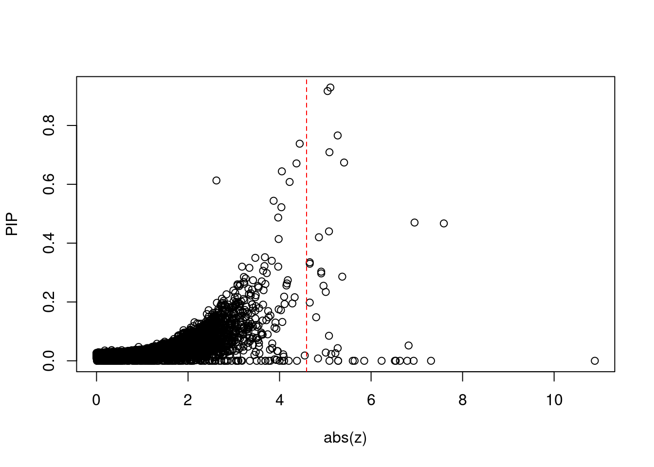

Version	Author	Date
3a7fbc1	wesleycrouse	2021-09-08

#proportion of significant z scores
mean(abs(ctwas_gene_res$z) > sig_thresh)

[1] 0.003458367

#genes with most significant z scores
head(ctwas_gene_res[order(-abs(ctwas_gene_res$z)),report_cols],20)

       genename region_tag susie_pip     mu2     PVE     z
9819   HLA-DQB1       6_26     0.000 1702.71 0.0e+00 10.89
6795      JAZF1       7_23     0.467   50.16 7.0e-05  7.59
11533      MICB       6_26     0.000  203.41 0.0e+00 -7.31
13639 LINC01126       2_27     0.470   39.52 5.5e-05  6.95
11765     DDAH2       6_26     0.000  249.28 0.0e+00  6.93
8540       TAP1       6_28     0.052   59.95 9.4e-06  6.82
11764     CLIC1       6_26     0.000  291.86 0.0e+00 -6.79
12473       C4A       6_26     0.000  315.89 0.0e+00  6.63
11506    ZBTB12       6_26     0.000  315.92 0.0e+00 -6.54
11526      APOM       6_26     0.000  308.81 0.0e+00  6.52
11518      MSH5       6_26     0.000  281.93 0.0e+00  6.23
11677     HCG27       6_26     0.000  131.49 0.0e+00 -5.85
11490    NOTCH4       6_26     0.000  290.52 0.0e+00  5.64
11962       C4B       6_26     0.000  202.41 0.0e+00 -5.60
9232      PEAK1      15_36     0.674   29.43 5.9e-05 -5.41
7087      AP3S2      15_41     0.286   27.26 2.3e-05 -5.37
11493      RNF5       6_26     0.000  426.06 0.0e+00  5.28
11933      PPT2       6_26     0.000  425.52 0.0e+00 -5.28
3953      RREB1        6_7     0.766   26.94 6.1e-05 -5.27
10742   NCR3LG1      11_12     0.043   26.71 3.4e-06  5.27

Locus plots for genes and SNPs

ctwas_gene_res_sortz <- ctwas_gene_res[order(-abs(ctwas_gene_res$z)),]

n_plots <- 5
for (region_tag_plot in head(unique(ctwas_gene_res_sortz$region_tag), n_plots)){
  ctwas_res_region <-  ctwas_res[ctwas_res$region_tag==region_tag_plot,]
  start <- min(ctwas_res_region$pos)
  end <- max(ctwas_res_region$pos)
  
  ctwas_res_region <- ctwas_res_region[order(ctwas_res_region$pos),]
  ctwas_res_region_gene <- ctwas_res_region[ctwas_res_region$type=="gene",]
  ctwas_res_region_snp <- ctwas_res_region[ctwas_res_region$type=="SNP",]
  
  #region name
  print(paste0("Region: ", region_tag_plot))
  
  #table of genes in region
  print(ctwas_res_region_gene[,report_cols])
  
  par(mfrow=c(4,1))
  
  #gene z scores
  plot(ctwas_res_region_gene$pos, abs(ctwas_res_region_gene$z), xlab="Position", ylab="abs(gene_z)", xlim=c(start,end),
   ylim=c(0,max(sig_thresh, abs(ctwas_res_region_gene$z))),
   main=paste0("Region: ", region_tag_plot))
  abline(h=sig_thresh,col="red",lty=2)
  
  #significance threshold for SNPs
  alpha_snp <- 5*10^(-8)
  sig_thresh_snp <- qnorm(1-alpha_snp/2, lower=T)
  
  #snp z scores
  plot(ctwas_res_region_snp$pos, abs(ctwas_res_region_snp$z), xlab="Position", ylab="abs(snp_z)",xlim=c(start,end),
   ylim=c(0,max(sig_thresh_snp, max(abs(ctwas_res_region_snp$z)))))
  abline(h=sig_thresh_snp,col="purple",lty=2)
  
  #gene pips
  plot(ctwas_res_region_gene$pos, ctwas_res_region_gene$susie_pip, xlab="Position", ylab="Gene PIP", xlim=c(start,end), ylim=c(0,1))
  abline(h=0.8,col="blue",lty=2)
  
  #snp pips
  plot(ctwas_res_region_snp$pos, ctwas_res_region_snp$susie_pip, xlab="Position", ylab="SNP PIP", xlim=c(start,end), ylim=c(0,1))
  abline(h=0.8,col="blue",lty=2)
}

[1] "Region: 6_26"
               genename region_tag susie_pip     mu2 PVE     z
11546              DDR1       6_26         0   52.51   0  3.60
11770            GTF2H4       6_26         0   75.54   0  4.38
5236              VARS2       6_26         0   25.02   0 -2.36
10913             SFTA2       6_26         0    6.90   0 -0.83
11539          PSORS1C1       6_26         0   66.71   0  4.10
11677             HCG27       6_26         0  131.49   0 -5.85
5226              TCF19       6_26         0   12.26   0 -1.46
11537            POU5F1       6_26         0   12.52   0 -1.49
11536             HLA-C       6_26         0   15.19   0 -1.71
12231             HLA-B       6_26         0    6.96   0 -0.84
13284 XXbac-BPG181B23.7       6_26         0    7.83   0 -0.97
11534              MICA       6_26         0   41.97   0 -3.18
11533              MICB       6_26         0  203.41   0 -7.31
11308            DDX39B       6_26         0   23.73   0 -2.28
11531           NFKBIL1       6_26         0   34.89   0  2.87
11516              VWA7       6_26         0   40.46   0 -0.22
12172               TNF       6_26         0   21.05   0  2.12
11530              LST1       6_26         0   46.10   0  3.35
11529              AIF1       6_26         0    5.04   0 -0.37
11527              BAG6       6_26         0    8.71   0  1.22
11523            GPANK1       6_26         0   13.82   0  2.46
11526              APOM       6_26         0  308.81   0  6.52
11524           C6orf47       6_26         0   29.36   0 -2.08
12350            LY6G5B       6_26         0   25.14   0  0.21
11521           ABHD16A       6_26         0   34.44   0 -1.06
11520            LY6G6C       6_26         0   30.73   0 -0.01
11765             DDAH2       6_26         0  249.28   0  6.93
11518              MSH5       6_26         0  281.93   0  6.23
11764             CLIC1       6_26         0  291.86   0 -6.79
12085            SAPCD1       6_26         0   31.15   0  1.73
11515              VARS       6_26         0   21.97   0  0.40
11514              LSM2       6_26         0   20.95   0 -0.53
11513            HSPA1L       6_26         0  133.50   0 -3.80
11511           C6orf48       6_26         0   47.17   0 -0.50
11510              NEU1       6_26         0   28.69   0 -1.80
11509           SLC44A4       6_26         0   67.86   0 -3.69
11506            ZBTB12       6_26         0  315.92   0 -6.54
11504            SKIV2L       6_26         0   72.51   0 -2.37
11502             STK19       6_26         0   43.15   0  2.68
11503               DXO       6_26         0   22.50   0  3.09
12473               C4A       6_26         0  315.89   0  6.63
11962               C4B       6_26         0  202.41   0 -5.60
11491              PBX2       6_26         0  134.25   0 -2.46
11759             ATF6B       6_26         0   49.30   0 -2.60
11497             FKBPL       6_26         0   90.99   0  0.53
11496             PRRT1       6_26         0   21.80   0  0.14
11933              PPT2       6_26         0  425.52   0 -5.28
12377             EGFL8       6_26         0  183.21   0  3.69
11494            AGPAT1       6_26         0   37.34   0 -4.00
11493              RNF5       6_26         0  426.06   0  5.28
11492              AGER       6_26         0  346.88   0 -5.09
11756             GPSM3       6_26         0   50.65   0  0.56
11490            NOTCH4       6_26         0  290.52   0  5.64
11488           HLA-DRA       6_26         0   82.90   0  4.06
10890          HLA-DRB1       6_26         0   78.97   0 -3.05
9819           HLA-DQB1       6_26         0 1702.71   0 10.89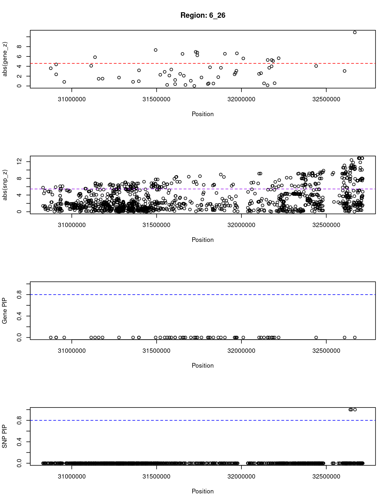

Version	Author	Date
3a7fbc1	wesleycrouse	2021-09-08

[1] "Region: 7_23"
           genename region_tag susie_pip   mu2     PVE     z
13201 CTD-2227E11.1       7_23     0.011  5.72 2.0e-07 -0.57
3758           CBX3       7_23     0.010  5.04 1.5e-07 -0.80
1204          SNX10       7_23     0.011  5.63 1.9e-07 -0.75
11850    AC004540.5       7_23     0.016  8.63 4.1e-07  1.24
3755       KIAA0087       7_23     0.060 20.04 3.6e-06  2.17
11140         HOXA4       7_23     0.013  6.60 2.5e-07 -0.66
2291          HOXA5       7_23     0.010  4.61 1.4e-07 -0.36
2299         HIBADH       7_23     0.012  6.22 2.2e-07  0.65
6795          JAZF1       7_23     0.467 50.16 7.0e-05  7.59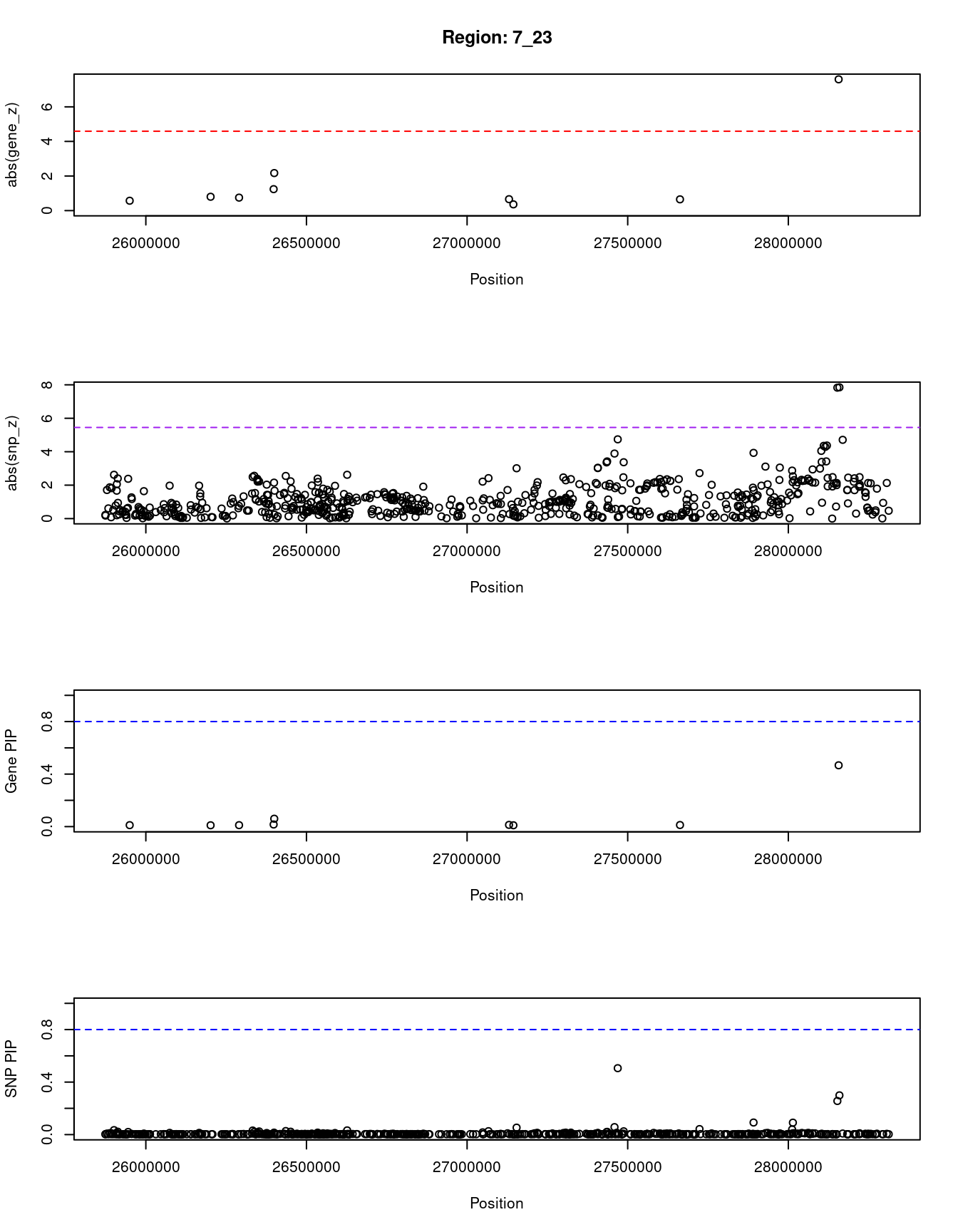

Version	Author	Date
3a7fbc1	wesleycrouse	2021-09-08

[1] "Region: 2_27"
        genename region_tag susie_pip   mu2     PVE     z
12118 AC093609.1       2_27     0.017  4.42 2.2e-07 -0.45
13639  LINC01126       2_27     0.470 39.52 5.5e-05  6.95
11946 C1GALT1C1L       2_27     0.017  4.65 2.4e-07  0.61
6708     PLEKHH2       2_27     0.017  4.36 2.2e-07  0.04
3229       THADA       2_27     0.019  5.36 3.1e-07  0.53
5330    DYNC2LI1       2_27     0.046 13.38 1.8e-06  1.86
5343      LRPPRC       2_27     0.038 11.86 1.3e-06  1.77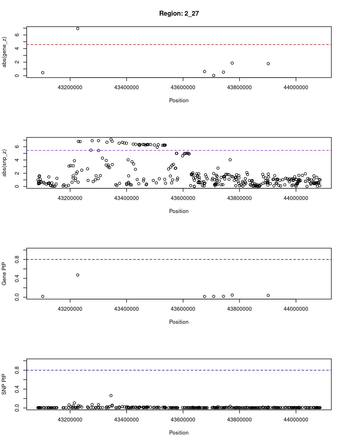

Version	Author	Date
3a7fbc1	wesleycrouse	2021-09-08

[1] "Region: 6_28"
       genename region_tag susie_pip   mu2     PVE     z
12370   HLA-DOB       6_28     0.003 41.33 3.8e-07 -2.27
11484 PSMB8-AS1       6_28     0.002 12.26 7.0e-08  0.83
11486     PSMB8       6_28     0.001  5.10 1.1e-08  0.41
12351     PSMB9       6_28     0.001  9.98 3.9e-08  0.71
8540       TAP1       6_28     0.052 59.95 9.4e-06  6.82
12410   HLA-DMB       6_28     0.003 24.98 1.9e-07 -3.93
11482      BRD2       6_28     0.001 11.50 3.4e-08  3.16
11483   HLA-DMA       6_28     0.003 26.32 2.3e-07 -3.93
11481   HLA-DOA       6_28     0.001  8.47 2.2e-08  2.38
11478      RXRB       6_28     0.001  9.28 3.9e-08  0.80
11480   COL11A2       6_28     0.001  5.28 1.1e-08  0.47
11477   HSD17B8       6_28     0.002 13.56 7.3e-08 -2.18
12038     WDR46       6_28     0.001  7.27 2.2e-08 -0.30
11942     VPS52       6_28     0.001  4.35 9.0e-09  0.06
12135     RPS18       6_28     0.001  5.11 1.2e-08 -0.56
12259   B3GALT4       6_28     0.001  4.97 1.1e-08  0.53
12300      RGL2       6_28     0.004 20.31 2.7e-07 -2.04
12147     TAPBP       6_28     0.001  5.24 1.2e-08 -0.61
12267    ZBTB22       6_28     0.001  5.71 1.4e-08 -0.45
11473      DAXX       6_28     0.001  8.77 2.9e-08  0.95
2901       CUTA       6_28     0.001  5.44 1.3e-08  0.64
341        BAK1       6_28     0.054 39.36 6.3e-06 -3.42
1477      ITPR3       6_28     0.001  4.36 9.0e-09  0.07
5224      UQCC2       6_28     0.001  5.21 1.2e-08 -0.22
7434      IP6K3       6_28     0.001  4.93 1.1e-08 -0.16
7435      LEMD2       6_28     0.001  5.01 1.2e-08  0.72
3918       GRM4       6_28     0.001  4.55 9.7e-09  0.21
13290     NUDT3       6_28     0.001 10.13 4.1e-08  1.24
3936      RPS10       6_28     0.002 11.45 5.8e-08  1.47
3941      SPDEF       6_28     0.001  4.40 9.2e-09 -0.16
11027  C6orf106       6_28     0.003 15.22 1.2e-07  1.77
3925      SNRPC       6_28     0.006 22.03 4.1e-07 -2.22
638       TAF11       6_28     0.001  5.00 1.1e-08 -0.37
6234     SCUBE3       6_28     0.004 17.79 1.9e-07  2.03
304        DEF6       6_28     0.001  4.85 1.1e-08  0.40
2846      PPARD       6_28     0.002 13.07 8.1e-08  1.69
11347    RPL10A       6_28     0.001  7.32 2.2e-08  0.94
2847      FANCE       6_28     0.002 11.46 5.6e-08 -1.46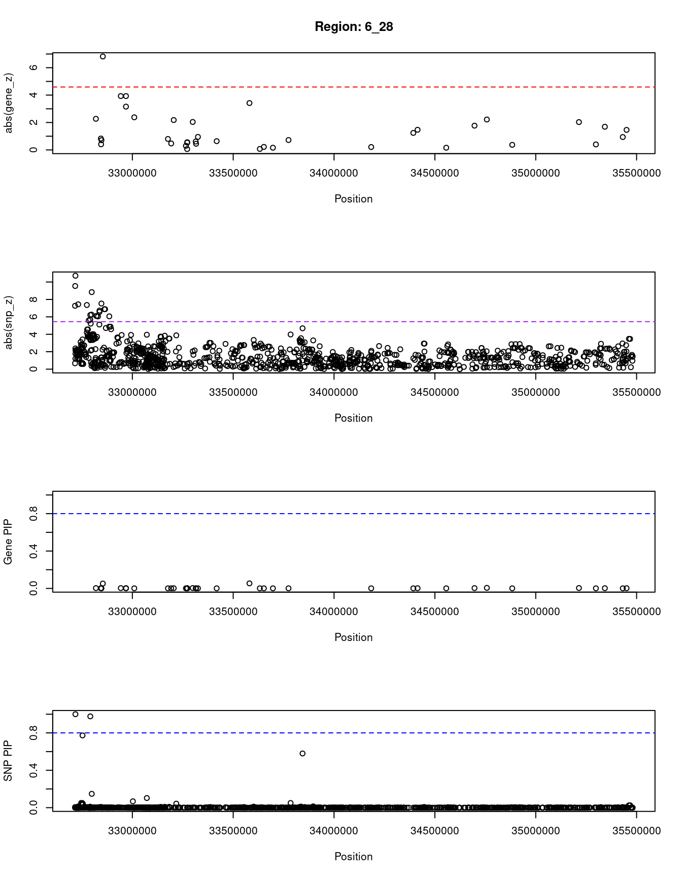

Version	Author	Date
3a7fbc1	wesleycrouse	2021-09-08

[1] "Region: 15_36"
          genename region_tag susie_pip   mu2     PVE     z
8733       TMEM266      15_36     0.009  4.55 1.3e-07  0.29
5606          ETFA      15_36     0.013  6.56 2.5e-07  0.44
5608        SCAPER      15_36     0.009  4.35 1.2e-07 -0.22
3413          RCN2      15_36     0.015  9.49 4.2e-07  1.24
5609        TSPAN3      15_36     0.010  5.63 1.7e-07 -0.56
9232         PEAK1      15_36     0.674 29.43 5.9e-05 -5.41
8737        LINGO1      15_36     0.010  4.59 1.3e-07  0.46
8334       TBC1D2B      15_36     0.010  4.62 1.3e-07 -0.69
10196        SH2D7      15_36     0.062 18.72 3.5e-06  2.96
12917 RP11-285A1.1      15_36     0.009  4.65 1.3e-07  0.54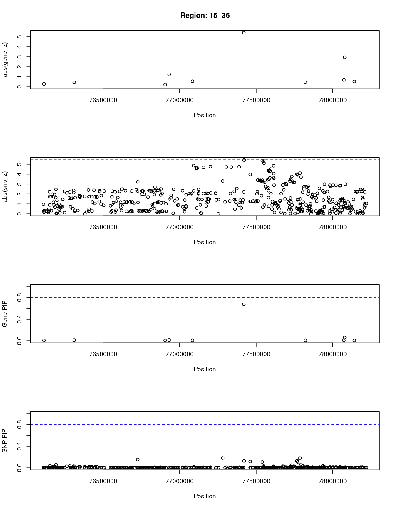

Version	Author	Date
3a7fbc1	wesleycrouse	2021-09-08

SNPs with highest PIPs

#snps with PIP>0.8 or 20 highest PIPs
head(ctwas_snp_res[order(-ctwas_snp_res$susie_pip),report_cols_snps],
max(sum(ctwas_snp_res$susie_pip>0.8), 20))

                id region_tag susie_pip     mu2     PVE     z
37018   rs75222047       1_85     1.000  668.28 2.0e-03  2.91
82161   rs12471681       2_53     1.000  783.82 2.3e-03 -3.05
140714  rs13062973       3_45     1.000  541.57 1.6e-03 -3.60
168715   rs1388475      3_107     1.000  444.68 1.3e-03  2.87
168716  rs13071192      3_107     1.000  424.11 1.3e-03 -3.12
171181  rs28661518      3_112     1.000  821.91 2.4e-03 -3.09
210999   rs2125449       4_79     1.000  856.32 2.5e-03 -3.33
254120   rs3910018       5_51     1.000  698.94 2.1e-03 -2.86
285519   rs2206734       6_15     1.000   82.48 2.5e-04 10.34
287817  rs34662244       6_22     1.000 1461.50 4.3e-03  4.07
287835  rs67297533       6_22     1.000 1426.13 4.2e-03 -4.09
290443   rs9272679       6_26     1.000 1600.39 4.8e-03 -9.31
290452  rs17612548       6_26     1.000 1678.40 5.0e-03 11.17
290473   rs3134996       6_26     1.000 1653.74 4.9e-03 10.37
290557   rs3916765       6_28     1.000  101.65 3.0e-04 10.72
381853   rs1495743       8_21     1.000  368.25 1.1e-03  3.21
409488  rs16902104       8_83     1.000 1075.01 3.2e-03  3.51
438361   rs7025746       9_53     1.000  336.14 1.0e-03 -3.04
438365   rs2900388       9_53     1.000  329.92 9.8e-04  3.51
473772   rs2019640      10_59     1.000  865.23 2.6e-03 -3.47
473774    rs913647      10_59     1.000  867.73 2.6e-03  3.45
479127  rs12244851      10_70     1.000  252.86 7.5e-04 22.39
486665    rs234856       11_2     1.000   36.37 1.1e-04 -4.94
488698  rs11041828       11_6     1.000  747.14 2.2e-03  2.96
488699   rs4237770       11_6     1.000  765.34 2.3e-03 -2.93
500638 rs113527193      11_30     1.000  421.58 1.3e-03  3.29
500969  rs11603701      11_30     1.000  404.06 1.2e-03 -3.24
569057   rs9526909      13_22     1.000  548.39 1.6e-03  2.54
615748  rs12912777      15_13     1.000   32.51 9.7e-05  5.53
652239  rs12443634      16_45     1.000  177.59 5.3e-04 -3.47
652246   rs2966092      16_45     1.000  180.00 5.3e-04  3.38
657767   rs4790233       17_5     1.000  187.07 5.6e-04 -3.70
657772   rs8072531       17_5     1.000  187.88 5.6e-04 -3.98
703424  rs73537429      19_16     1.000  240.26 7.1e-04 -2.52
722820   rs2747568      20_20     1.000 1126.85 3.3e-03  3.79
722821   rs2064505      20_20     1.000 1158.08 3.4e-03 -3.92
65949     rs780093       2_16     0.999   41.72 1.2e-04  6.98
431679   rs9410573       9_40     0.999   46.55 1.4e-04 -7.44
664657   rs9906451      17_22     0.999   30.18 9.0e-05 -5.87
703453   rs2285626      19_16     0.995  106.84 3.2e-04  5.36
576877   rs1327315      13_40     0.994   32.42 9.6e-05 -7.40
381856  rs34537991       8_21     0.988  318.16 9.3e-04  3.06
422967  rs10965243       9_16     0.988   26.01 7.6e-05 -5.41
290658   rs2857161       6_28     0.977   87.90 2.6e-04  6.21
47621   rs79687284      1_108     0.974   25.20 7.3e-05  5.66
438364   rs7868850       9_53     0.972   62.75 1.8e-04  0.83
703426  rs67238925      19_16     0.971  231.16 6.7e-04  2.39
438362   rs4742930       9_53     0.964  261.59 7.5e-04  3.25
168718  rs13081434      3_107     0.952  405.99 1.1e-03 -2.47
540158    rs189339      12_40     0.938   32.96 9.2e-05 -6.27
486664    rs234852       11_2     0.936   25.44 7.1e-05  3.12
29222    rs6679677       1_70     0.935   25.86 7.2e-05  5.33
409487  rs16902103       8_83     0.933 1049.15 2.9e-03 -3.50
155021  rs72964564       3_76     0.929   32.69 9.0e-05 -6.10
473852   rs1977833      10_59     0.925   93.99 2.6e-04 -8.47
171182  rs73190822      3_112     0.917  801.36 2.2e-03  3.11
257315  rs10479168       5_59     0.908   25.97 7.0e-05  5.36
576889    rs502027      13_40     0.907   31.45 8.5e-05  7.22
491339      rs5215      11_12     0.865   35.91 9.2e-05 -6.41
205552  rs35518360       4_67     0.863   24.41 6.3e-05  4.70
649482  rs72802395      16_40     0.862   35.19 9.0e-05 -6.35
177657   rs1801212        4_7     0.861   56.52 1.4e-04  8.59
537207   rs2682323      12_33     0.858   24.00 6.1e-05  4.74
47625     rs340835      1_108     0.847   25.68 6.5e-05  5.52
37037    rs2179109       1_85     0.844  688.12 1.7e-03 -3.03
139980   rs3774723       3_43     0.824   24.64 6.0e-05 -4.84
171180  rs62287225      3_112     0.821  801.11 2.0e-03  3.08
140702  rs34695932       3_45     0.814  568.29 1.4e-03  4.13
657763  rs79425343       17_5     0.808   23.29 5.6e-05  1.15
608779  rs11160254      14_49     0.805   24.26 5.8e-05  4.55
710481  rs12609461      19_33     0.802   28.75 6.9e-05  5.53

SNPs with largest effect sizes

#plot PIP vs effect size
plot(ctwas_snp_res$susie_pip, ctwas_snp_res$mu2, xlab="PIP", ylab="mu^2", main="SNP PIPs vs Effect Size")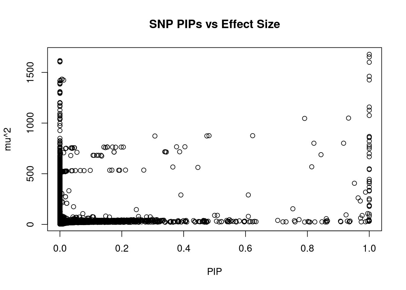

Version	Author	Date
3a7fbc1	wesleycrouse	2021-09-08

#SNPs with 50 largest effect sizes
head(ctwas_snp_res[order(-ctwas_snp_res$mu2),report_cols_snps],50)

               id region_tag susie_pip     mu2     PVE     z
290452 rs17612548       6_26     1.000 1678.40 5.0e-03 11.17
290473  rs3134996       6_26     1.000 1653.74 4.9e-03 10.37
290451 rs17612510       6_26     0.000 1616.59 1.8e-08 10.42
290459  rs9273524       6_26     0.000 1609.01 0.0e+00 10.93
290453 rs17612633       6_26     0.000 1607.91 0.0e+00 10.90
290450  rs9273242       6_26     0.000 1603.82 0.0e+00 10.58
290443  rs9272679       6_26     1.000 1600.39 4.8e-03 -9.31
287817 rs34662244       6_22     1.000 1461.50 4.3e-03  4.07
287872 rs13191786       6_22     0.007 1432.89 2.8e-05  4.10
287875 rs34218844       6_22     0.006 1432.64 2.4e-05  4.09
287835 rs67297533       6_22     1.000 1426.13 4.2e-03 -4.09
287861 rs67998226       6_22     0.012 1423.82 5.3e-05  4.25
287880 rs35030260       6_22     0.001 1421.93 4.1e-06  4.12
287866 rs33932084       6_22     0.000 1416.75 5.2e-08  3.93
287885 rs13198809       6_22     0.000 1398.05 1.0e-08  4.08
287894 rs36092177       6_22     0.000 1391.64 2.4e-09  4.08
287919 rs55690788       6_22     0.000 1385.19 2.3e-09  4.16
288031  rs1311917       6_22     0.000 1309.74 4.3e-19  3.82
288023  rs1233611       6_22     0.000 1308.69 0.0e+00  3.78
288041  rs9257192       6_22     0.000 1301.84 4.3e-19  3.92
288055  rs3135297       6_22     0.000 1301.17 4.3e-19  3.93
288060  rs9257267       6_22     0.000 1300.87 0.0e+00  3.90
288077  rs3130838       6_22     0.000 1292.94 0.0e+00  3.95
290357  rs9270587       6_26     0.000 1202.04 0.0e+00  9.14
290361  rs9270624       6_26     0.000 1199.33 0.0e+00  9.09
290368  rs9270865       6_26     0.000 1198.60 0.0e+00  9.09
290371  rs9270971       6_26     0.000 1198.21 0.0e+00  9.09
290379  rs9271108       6_26     0.000 1198.04 0.0e+00  9.09
290382  rs9271192       6_26     0.000 1197.99 0.0e+00  9.09
290387  rs9271260       6_26     0.000 1197.93 0.0e+00  9.09
290385  rs9271247       6_26     0.000 1197.57 0.0e+00  9.08
290377  rs9271092       6_26     0.000 1197.39 0.0e+00  9.07
290383  rs9271202       6_26     0.000 1197.32 0.0e+00  9.07
290455 rs17612852       6_26     0.000 1174.58 0.0e+00 10.40
290454 rs17612712       6_26     0.000 1163.89 0.0e+00 12.39
722821  rs2064505      20_20     1.000 1158.08 3.4e-03 -3.92
290551  rs3104407       6_26     0.000 1127.83 0.0e+00  7.92
722820  rs2747568      20_20     1.000 1126.85 3.3e-03  3.79
287991  rs9393925       6_22     0.000 1092.81 0.0e+00 -3.66
290456  rs9273354       6_26     0.000 1092.01 0.0e+00 11.78
290474  rs3134994       6_26     0.000 1076.28 0.0e+00 10.28
409488 rs16902104       8_83     1.000 1075.01 3.2e-03  3.51
290468  rs3830058       6_26     0.000 1068.07 0.0e+00 10.17
290514  rs3135190       6_26     0.000 1049.67 0.0e+00  9.99
409487 rs16902103       8_83     0.933 1049.15 2.9e-03 -3.50
409485 rs34585331       8_83     0.791 1045.96 2.5e-03 -3.55
287837  rs9380064       6_22     0.000 1040.79 0.0e+00  4.03
287822  rs4713140       6_22     0.000 1039.54 0.0e+00  4.03
290537  rs3129726       6_26     0.000 1036.37 0.0e+00 10.03
287865  rs6905391       6_22     0.000  996.72 0.0e+00  4.43

SNPs with highest PVE

#SNPs with 50 highest pve
head(ctwas_snp_res[order(-ctwas_snp_res$PVE),report_cols_snps],50)

                id region_tag susie_pip     mu2     PVE     z
290452  rs17612548       6_26     1.000 1678.40 0.00500 11.17
290473   rs3134996       6_26     1.000 1653.74 0.00490 10.37
290443   rs9272679       6_26     1.000 1600.39 0.00480 -9.31
287817  rs34662244       6_22     1.000 1461.50 0.00430  4.07
287835  rs67297533       6_22     1.000 1426.13 0.00420 -4.09
722821   rs2064505      20_20     1.000 1158.08 0.00340 -3.92
722820   rs2747568      20_20     1.000 1126.85 0.00330  3.79
409488  rs16902104       8_83     1.000 1075.01 0.00320  3.51
409487  rs16902103       8_83     0.933 1049.15 0.00290 -3.50
473772   rs2019640      10_59     1.000  865.23 0.00260 -3.47
473774    rs913647      10_59     1.000  867.73 0.00260  3.45
210999   rs2125449       4_79     1.000  856.32 0.00250 -3.33
409485  rs34585331       8_83     0.791 1045.96 0.00250 -3.55
171181  rs28661518      3_112     1.000  821.91 0.00240 -3.09
82161   rs12471681       2_53     1.000  783.82 0.00230 -3.05
488699   rs4237770       11_6     1.000  765.34 0.00230 -2.93
171182  rs73190822      3_112     0.917  801.36 0.00220  3.11
488698  rs11041828       11_6     1.000  747.14 0.00220  2.96
254120   rs3910018       5_51     1.000  698.94 0.00210 -2.86
37018   rs75222047       1_85     1.000  668.28 0.00200  2.91
171180  rs62287225      3_112     0.821  801.11 0.00200  3.08
37037    rs2179109       1_85     0.844  688.12 0.00170 -3.03
140714  rs13062973       3_45     1.000  541.57 0.00160 -3.60
211019  rs11721784       4_79     0.623  875.57 0.00160  3.38
569057   rs9526909      13_22     1.000  548.39 0.00160  2.54
140702  rs34695932       3_45     0.814  568.29 0.00140  4.13
168715   rs1388475      3_107     1.000  444.68 0.00130  2.87
168716  rs13071192      3_107     1.000  424.11 0.00130 -3.12
211006   rs1542437       4_79     0.482  875.79 0.00130  3.35
500638 rs113527193      11_30     1.000  421.58 0.00130  3.29
210985  rs13109930       4_79     0.475  873.05 0.00120  3.11
500969  rs11603701      11_30     1.000  404.06 0.00120 -3.24
168718  rs13081434      3_107     0.952  405.99 0.00110 -2.47
381853   rs1495743       8_21     1.000  368.25 0.00110  3.21
438361   rs7025746       9_53     1.000  336.14 0.00100 -3.04
438365   rs2900388       9_53     1.000  329.92 0.00098  3.51
381856  rs34537991       8_21     0.988  318.16 0.00093  3.06
82157   rs75755471       2_53     0.404  765.93 0.00092  3.07
82163   rs78406274       2_53     0.377  765.82 0.00086  3.06
254131  rs10805847       5_51     0.387  716.82 0.00082  2.87
210987   rs6819187       4_79     0.307  872.37 0.00080  3.09
438362   rs4742930       9_53     0.964  261.59 0.00075  3.25
479127  rs12244851      10_70     1.000  252.86 0.00075 22.39
140708  rs13071831       3_45     0.446  562.30 0.00074  4.15
254107  rs10064286       5_51     0.344  714.09 0.00073 -2.93
254125   rs3910025       5_51     0.341  716.64 0.00073  2.86
254126   rs3902731       5_51     0.339  716.64 0.00072  2.86
703424  rs73537429      19_16     1.000  240.26 0.00071 -2.52
703426  rs67238925      19_16     0.971  231.16 0.00067  2.39
140705  rs13077334       3_45     0.365  566.50 0.00061  4.07

SNPs with largest z scores

#SNPs with 50 largest z scores
head(ctwas_snp_res[order(-abs(ctwas_snp_res$z)),report_cols_snps],50)

               id region_tag susie_pip     mu2     PVE     z
479135 rs12260037      10_70     0.007  226.58 4.9e-06 22.65
479127 rs12244851      10_70     1.000  252.86 7.5e-04 22.39
479124  rs6585198      10_70     0.001  125.48 5.4e-07 15.56
479136 rs12359102      10_70     0.001   95.62 2.0e-07 14.81
479134  rs7077039      10_70     0.001   95.36 2.0e-07 14.79
479132  rs7921525      10_70     0.001   92.04 2.0e-07 14.58
479140  rs4077527      10_70     0.001   86.67 1.9e-07 14.57
479133  rs6585203      10_70     0.001   91.12 2.0e-07 14.52
479129 rs11196191      10_70     0.001   90.94 2.0e-07 14.51
479130 rs10787472      10_70     0.001   90.51 2.0e-07 14.49
290495  rs9275221       6_26     0.000  347.96 0.0e+00 12.84
290546  rs9275583       6_26     0.000  348.06 0.0e+00 12.83
290503  rs9275275       6_26     0.000  346.54 0.0e+00 12.82
290508  rs9275307       6_26     0.000  346.83 0.0e+00 12.82
290539  rs4273728       6_26     0.000  346.89 0.0e+00 12.82
290497  rs9275223       6_26     0.000  346.36 0.0e+00 12.81
290454 rs17612712       6_26     0.000 1163.89 0.0e+00 12.39
479118 rs12243578      10_70     0.003   79.91 6.7e-07 12.36
290515  rs9275362       6_26     0.000  180.04 0.0e+00 11.83
290456  rs9273354       6_26     0.000 1092.01 0.0e+00 11.78
290452 rs17612548       6_26     1.000 1678.40 5.0e-03 11.17
290375   rs617578       6_26     0.000  254.37 0.0e+00 11.10
290459  rs9273524       6_26     0.000 1609.01 0.0e+00 10.93
290453 rs17612633       6_26     0.000 1607.91 0.0e+00 10.90
290471  rs3828800       6_26     0.000  263.49 0.0e+00 10.83
290460  rs9273528       6_26     0.000  231.14 0.0e+00 10.73
290557  rs3916765       6_28     1.000  101.65 3.0e-04 10.72
290444 rs34763586       6_26     0.000  428.60 0.0e+00 10.63
290462 rs28724252       6_26     0.000  228.10 0.0e+00 10.61
290450  rs9273242       6_26     0.000 1603.82 0.0e+00 10.58
290363  rs2760985       6_26     0.000  403.54 0.0e+00 10.56
171760 rs11929397      3_114     0.509   89.36 1.4e-04 10.55
171761 rs11716713      3_114     0.500   89.31 1.3e-04 10.55
290369  rs2647066       6_26     0.000  403.02 0.0e+00 10.52
290518  rs3135002       6_26     0.000  974.60 0.0e+00 10.51
290388  rs3997872       6_26     0.000  403.83 0.0e+00 10.48
290451 rs17612510       6_26     0.000 1616.59 1.8e-08 10.42
290455 rs17612852       6_26     0.000 1174.58 0.0e+00 10.40
290473  rs3134996       6_26     1.000 1653.74 4.9e-03 10.37
285519  rs2206734       6_15     1.000   82.48 2.5e-04 10.34
290474  rs3134994       6_26     0.000 1076.28 0.0e+00 10.28
290468  rs3830058       6_26     0.000 1068.07 0.0e+00 10.17
290537  rs3129726       6_26     0.000 1036.37 0.0e+00 10.03
290514  rs3135190       6_26     0.000 1049.67 0.0e+00  9.99
290348 rs12191360       6_26     0.000  431.38 0.0e+00  9.85
290441 rs41269945       6_26     0.000  420.19 0.0e+00  9.81
290399  rs3129757       6_26     0.000  714.79 0.0e+00  9.56
644109 rs79994966      16_29     0.292   74.31 6.5e-05  9.56
644105 rs17817712      16_29     0.280   74.18 6.2e-05  9.55
290398  rs9271347       6_26     0.000  714.04 0.0e+00  9.54

Gene set enrichment for genes with PIP>0.8

#GO enrichment analysis
library(enrichR)

Welcome to enrichR
Checking connection ...

Enrichr ... Connection is Live!
FlyEnrichr ... Connection is available!
WormEnrichr ... Connection is available!
YeastEnrichr ... Connection is available!
FishEnrichr ... Connection is available!

dbs <- c("GO_Biological_Process_2021", "GO_Cellular_Component_2021", "GO_Molecular_Function_2021")
genes <- ctwas_gene_res$genename[ctwas_gene_res$susie_pip>0.8]

#number of genes for gene set enrichment
length(genes)

[1] 2

if (length(genes)>0){
  GO_enrichment <- enrichr(genes, dbs)

  for (db in dbs){
    print(db)
    df <- GO_enrichment[[db]]
    df <- df[df$Adjusted.P.value<0.05,c("Term", "Overlap", "Adjusted.P.value", "Genes")]
    print(df)
  }
  
  #DisGeNET enrichment
  
  # devtools::install_bitbucket("ibi_group/disgenet2r")
  library(disgenet2r)
  
  disgenet_api_key <- get_disgenet_api_key(
                    email = "wesleycrouse@gmail.com", 
                    password = "uchicago1" )
  
  Sys.setenv(DISGENET_API_KEY= disgenet_api_key)
  
  res_enrich <-disease_enrichment(entities=genes, vocabulary = "HGNC",
                               database = "CURATED" )
  
  df <- res_enrich@qresult[1:10, c("Description", "FDR", "Ratio",  "BgRatio")]
  print(df)
  
  #WebGestalt enrichment
  library(WebGestaltR)
  
  background <- ctwas_gene_res$genename
  
  #listGeneSet()
  databases <- c("pathway_KEGG", "disease_GLAD4U", "disease_OMIM")
  
  enrichResult <- WebGestaltR(enrichMethod="ORA", organism="hsapiens",
                              interestGene=genes, referenceGene=background,
                              enrichDatabase=databases, interestGeneType="genesymbol",
                              referenceGeneType="genesymbol", isOutput=F)
  print(enrichResult[,c("description", "size", "overlap", "FDR", "database", "userId")])
}

Uploading data to Enrichr... Done.
  Querying GO_Biological_Process_2021... Done.
  Querying GO_Cellular_Component_2021... Done.
  Querying GO_Molecular_Function_2021... Done.
Parsing results... Done.
[1] "GO_Biological_Process_2021"
                                                                    Term
1                       peptidyl-serine autophosphorylation (GO:0036289)
2                    negative regulation of hippo signaling (GO:0035331)
3                             regulation of hippo signaling (GO:0035330)
4                    positive regulation of protein binding (GO:0032092)
5         negative regulation of blood vessel morphogenesis (GO:2000181)
6                       negative regulation of angiogenesis (GO:0016525)
7                            positive regulation of binding (GO:0051099)
8                             regulation of protein binding (GO:0043393)
9                           peptidyl-serine phosphorylation (GO:0018105)
10                              protein autophosphorylation (GO:0046777)
11                             peptidyl-serine modification (GO:0018209)
12 negative regulation of intracellular signal transduction (GO:1902532)
13                               regulation of angiogenesis (GO:0045765)
14                                             MAPK cascade (GO:0000165)
15                       transcription by RNA polymerase II (GO:0006366)
16                                          phosphorylation (GO:0016310)
   Overlap Adjusted.P.value Genes
1      1/8       0.01169624 MARK3
2     1/13       0.01169624 MARK3
3     1/20       0.01199408 MARK3
4     1/58       0.02309111 MARK3
5     1/78       0.02309111 GTF2I
6     1/87       0.02309111 GTF2I
7     1/90       0.02309111 MARK3
8    1/118       0.02647208 MARK3
9    1/156       0.02753817 MARK3
10   1/159       0.02753817 MARK3
11   1/169       0.02753817 MARK3
12   1/198       0.02796553 MARK3
13   1/203       0.02796553 GTF2I
14   1/303       0.03809352 MARK3
15   1/320       0.03809352 GTF2I
16   1/400       0.04455087 MARK3
[1] "GO_Cellular_Component_2021"
[1] Term             Overlap          Adjusted.P.value Genes           
<0 rows> (or 0-length row.names)
[1] "GO_Molecular_Function_2021"
                                                                                   Term
1                                              tau-protein kinase activity (GO:0050321)
2                                                      tau protein binding (GO:0048156)
3      RNA polymerase II-specific DNA-binding transcription factor binding (GO:0061629)
4                                 DNA-binding transcription factor binding (GO:0140297)
5 DNA-binding transcription activator activity, RNA polymerase II-specific (GO:0001228)
6                                 protein serine/threonine kinase activity (GO:0004674)
  Overlap Adjusted.P.value Genes
1    1/20       0.01198812 MARK3
2    1/40       0.01198812 MARK3
3   1/190       0.03103830 GTF2I
4   1/208       0.03103830 GTF2I
5   1/333       0.03410481 GTF2I
6   1/344       0.03410481 MARK3
                                        Description         FDR Ratio
7                           Thymic epithelial tumor 0.001339930   1/2
13 VISUAL IMPAIRMENT AND PROGRESSIVE PHTHISIS BULBI 0.001339930   1/2
4                                    Sicca Syndrome 0.006963326   1/2
5                                 Williams Syndrome 0.006963326   1/2
9                                Sjogren's Syndrome 0.006963326   1/2
1                               Atrial Fibrillation 0.035346597   1/2
2                       Leukemia, Myelocytic, Acute 0.035346597   1/2
3                        Acute Myeloid Leukemia, M1 0.035346597   1/2
6                    Paroxysmal atrial fibrillation 0.035346597   1/2
8                         Autism Spectrum Disorders 0.035346597   1/2
    BgRatio
7    1/9703
13   1/9703
4   13/9703
5    8/9703
9   13/9703
1  160/9703
2  173/9703
3  125/9703
6  156/9703
8   85/9703

******************************************

*                                        *

*          Welcome to WebGestaltR !      *

*                                        *

******************************************

Loading the functional categories...
Loading the ID list...
Loading the reference list...
Performing the enrichment analysis...

Warning in oraEnrichment(interestGeneList, referenceGeneList, geneSet,
minNum = minNum, : No significant gene set is identified based on FDR 0.05!

NULL

Sensitivity, specificity and precision for silver standard genes

library("readxl")

known_annotations <- read_xlsx("data/summary_known_genes_annotations.xlsx", sheet="T2D")
known_annotations <- unique(known_annotations$`Gene Symbol`)

unrelated_genes <- ctwas_gene_res$genename[!(ctwas_gene_res$genename %in% known_annotations)]

#number of genes in known annotations
print(length(known_annotations))

[1] 72

#number of genes in known annotations with imputed expression
print(sum(known_annotations %in% ctwas_gene_res$genename))

[1] 40

#assign ctwas, TWAS, and bystander genes
ctwas_genes <- ctwas_gene_res$genename[ctwas_gene_res$susie_pip>0.8]
twas_genes <- ctwas_gene_res$genename[abs(ctwas_gene_res$z)>sig_thresh]
novel_genes <- ctwas_genes[!(ctwas_genes %in% twas_genes)]

#significance threshold for TWAS
print(sig_thresh)

[1] 4.589937

#number of ctwas genes
length(ctwas_genes)

[1] 2

#number of TWAS genes
length(twas_genes)

[1] 39

#show novel genes (ctwas genes with not in TWAS genes)
ctwas_gene_res[ctwas_gene_res$genename %in% novel_genes,report_cols]

[1] genename   region_tag susie_pip  mu2        PVE        z         
<0 rows> (or 0-length row.names)

#sensitivity / recall
sensitivity <- rep(NA,2)
names(sensitivity) <- c("ctwas", "TWAS")
sensitivity["ctwas"] <- sum(ctwas_genes %in% known_annotations)/length(known_annotations)
sensitivity["TWAS"] <- sum(twas_genes %in% known_annotations)/length(known_annotations)
sensitivity

     ctwas       TWAS 
0.00000000 0.02777778

#specificity
specificity <- rep(NA,2)
names(specificity) <- c("ctwas", "TWAS")
specificity["ctwas"] <- sum(!(unrelated_genes %in% ctwas_genes))/length(unrelated_genes)
specificity["TWAS"] <- sum(!(unrelated_genes %in% twas_genes))/length(unrelated_genes)
specificity

    ctwas      TWAS 
0.9998220 0.9967073

#precision / PPV
precision <- rep(NA,2)
names(precision) <- c("ctwas", "TWAS")
precision["ctwas"] <- sum(ctwas_genes %in% known_annotations)/length(ctwas_genes)
precision["TWAS"] <- sum(twas_genes %in% known_annotations)/length(twas_genes)
precision

     ctwas       TWAS 
0.00000000 0.05128205

#ROC curves

pip_range <- (0:1000)/1000
sensitivity <- rep(NA, length(pip_range))
specificity <- rep(NA, length(pip_range))

for (index in 1:length(pip_range)){
  pip <- pip_range[index]
  ctwas_genes <- ctwas_gene_res$genename[ctwas_gene_res$susie_pip>=pip]
  sensitivity[index] <- sum(ctwas_genes %in% known_annotations)/length(known_annotations)
  specificity[index] <- sum(!(unrelated_genes %in% ctwas_genes))/length(unrelated_genes)
}

plot(1-specificity, sensitivity, type="l", xlim=c(0,1), ylim=c(0,1))

sig_thresh_range <- seq(from=0, to=max(abs(ctwas_gene_res$z)), length.out=length(pip_range))

for (index in 1:length(sig_thresh_range)){
  sig_thresh_plot <- sig_thresh_range[index]
  twas_genes <- ctwas_gene_res$genename[abs(ctwas_gene_res$z)>=sig_thresh_plot]
  sensitivity[index] <- sum(twas_genes %in% known_annotations)/length(known_annotations)
  specificity[index] <- sum(!(unrelated_genes %in% twas_genes))/length(unrelated_genes)
}

lines(1-specificity, sensitivity, xlim=c(0,1), ylim=c(0,1), col="red", lty=2)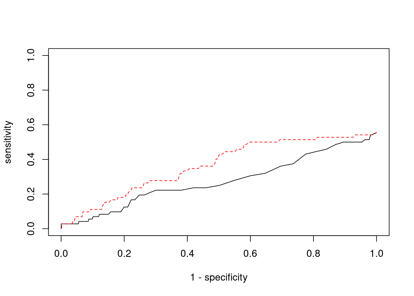

Version	Author	Date
3a7fbc1	wesleycrouse	2021-09-08

Sensitivity, specificity and precision for silver standard genes - bystanders only

This section first uses all silver standard genes to identify bystander genes within 1Mb. The silver standard and bystander gene lists are then subset to only genes with imputed expression in this analysis. Then, the ctwas and TWAS gene lists from this analysis are subset to only genes that are in the (subset) silver standard and bystander genes. These gene lists are then used to compute sensitivity, specificity and precision for ctwas and TWAS.

library(biomaRt)
library(GenomicRanges)

Loading required package: stats4

Loading required package: BiocGenerics

Loading required package: parallel


Attaching package: 'BiocGenerics'

The following objects are masked from 'package:parallel':

    clusterApply, clusterApplyLB, clusterCall, clusterEvalQ,
    clusterExport, clusterMap, parApply, parCapply, parLapply,
    parLapplyLB, parRapply, parSapply, parSapplyLB

The following objects are masked from 'package:stats':

    IQR, mad, sd, var, xtabs

The following objects are masked from 'package:base':

    anyDuplicated, append, as.data.frame, basename, cbind,
    colnames, dirname, do.call, duplicated, eval, evalq, Filter,
    Find, get, grep, grepl, intersect, is.unsorted, lapply, Map,
    mapply, match, mget, order, paste, pmax, pmax.int, pmin,
    pmin.int, Position, rank, rbind, Reduce, rownames, sapply,
    setdiff, sort, table, tapply, union, unique, unsplit, which,
    which.max, which.min

Loading required package: S4Vectors


Attaching package: 'S4Vectors'

The following object is masked from 'package:base':

    expand.grid

Loading required package: IRanges

Loading required package: GenomeInfoDb

ensembl <- useEnsembl(biomart="ENSEMBL_MART_ENSEMBL", dataset="hsapiens_gene_ensembl")
G_list <- getBM(filters= "chromosome_name", attributes= c("hgnc_symbol","chromosome_name","start_position","end_position","gene_biotype"), values=1:22, mart=ensembl)
G_list <- G_list[G_list$hgnc_symbol!="",]
G_list <- G_list[G_list$gene_biotype %in% c("protein_coding","lncRNA"),]
G_list$start <- G_list$start_position
G_list$end <- G_list$end_position
G_list_granges <- makeGRangesFromDataFrame(G_list, keep.extra.columns=T)

known_annotations_positions <- G_list[G_list$hgnc_symbol %in% known_annotations,]
half_window <- 1000000
known_annotations_positions$start <- known_annotations_positions$start_position - half_window
known_annotations_positions$end <- known_annotations_positions$end_position + half_window
known_annotations_positions$start[known_annotations_positions$start<1] <- 1
known_annotations_granges <- makeGRangesFromDataFrame(known_annotations_positions, keep.extra.columns=T)

bystanders <- findOverlaps(known_annotations_granges,G_list_granges)
bystanders <- unique(subjectHits(bystanders))
bystanders <- G_list$hgnc_symbol[bystanders]
bystanders <- bystanders[!(bystanders %in% known_annotations)]
unrelated_genes <- bystanders

#number of genes in known annotations
print(length(known_annotations))

[1] 72

#number of genes in known annotations with imputed expression
print(sum(known_annotations %in% ctwas_gene_res$genename))

[1] 40

#number of bystander genes
print(length(unrelated_genes))

[1] 1837

#number of bystander genes with imputed expression
print(sum(unrelated_genes %in% ctwas_gene_res$genename))

[1] 893

#remove genes without imputed expression from gene lists
known_annotations <- known_annotations[known_annotations %in% ctwas_gene_res$genename]
unrelated_genes <- unrelated_genes[unrelated_genes %in% ctwas_gene_res$genename]

#assign ctwas and TWAS genes
ctwas_genes <- ctwas_gene_res$genename[ctwas_gene_res$susie_pip>0.8]
twas_genes <- ctwas_gene_res$genename[abs(ctwas_gene_res$z)>sig_thresh]

#significance threshold for TWAS
print(sig_thresh)

[1] 4.589937

#number of ctwas genes
length(ctwas_genes)

[1] 2

#number of ctwas genes in known annotations or bystanders
sum(ctwas_genes %in% c(known_annotations, unrelated_genes))

[1] 0

#number of ctwas genes
length(twas_genes)

[1] 39

#number of TWAS genes
sum(twas_genes %in% c(known_annotations, unrelated_genes))

[1] 6

#remove genes not in known or bystander lists from results
ctwas_genes <- ctwas_genes[ctwas_genes %in% c(known_annotations, unrelated_genes)]
twas_genes <- twas_genes[twas_genes %in% c(known_annotations, unrelated_genes)]

#sensitivity / recall
sensitivity <- rep(NA,2)
names(sensitivity) <- c("ctwas", "TWAS")
sensitivity["ctwas"] <- sum(ctwas_genes %in% known_annotations)/length(known_annotations)
sensitivity["TWAS"] <- sum(twas_genes %in% known_annotations)/length(known_annotations)
sensitivity

ctwas  TWAS 
 0.00  0.05

#specificity
specificity <- rep(NA,2)
names(specificity) <- c("ctwas", "TWAS")
specificity["ctwas"] <- sum(!(unrelated_genes %in% ctwas_genes))/length(unrelated_genes)
specificity["TWAS"] <- sum(!(unrelated_genes %in% twas_genes))/length(unrelated_genes)
specificity

    ctwas      TWAS 
1.0000000 0.9955207

#precision / PPV
precision <- rep(NA,2)
names(precision) <- c("ctwas", "TWAS")
precision["ctwas"] <- sum(ctwas_genes %in% known_annotations)/length(ctwas_genes)
precision["TWAS"] <- sum(twas_genes %in% known_annotations)/length(twas_genes)
precision

    ctwas      TWAS 
      NaN 0.3333333

sessionInfo()

R version 3.6.1 (2019-07-05)
Platform: x86_64-pc-linux-gnu (64-bit)
Running under: Scientific Linux 7.4 (Nitrogen)

Matrix products: default
BLAS/LAPACK: /software/openblas-0.2.19-el7-x86_64/lib/libopenblas_haswellp-r0.2.19.so

locale:
 [1] LC_CTYPE=en_US.UTF-8       LC_NUMERIC=C              
 [3] LC_TIME=en_US.UTF-8        LC_COLLATE=en_US.UTF-8    
 [5] LC_MONETARY=en_US.UTF-8    LC_MESSAGES=en_US.UTF-8   
 [7] LC_PAPER=en_US.UTF-8       LC_NAME=C                 
 [9] LC_ADDRESS=C               LC_TELEPHONE=C            
[11] LC_MEASUREMENT=en_US.UTF-8 LC_IDENTIFICATION=C       

attached base packages:
[1] parallel  stats4    stats     graphics  grDevices utils     datasets 
[8] methods   base     

other attached packages:
 [1] GenomicRanges_1.36.0 GenomeInfoDb_1.20.0  IRanges_2.18.1      
 [4] S4Vectors_0.22.1     BiocGenerics_0.30.0  biomaRt_2.40.1      
 [7] readxl_1.3.1         WebGestaltR_0.4.4    disgenet2r_0.99.2   
[10] enrichR_3.0          cowplot_1.0.0        ggplot2_3.3.3       

loaded via a namespace (and not attached):
 [1] bitops_1.0-6           fs_1.3.1               bit64_4.0.5           
 [4] doParallel_1.0.16      progress_1.2.2         httr_1.4.1            
 [7] rprojroot_2.0.2        tools_3.6.1            doRNG_1.8.2           
[10] utf8_1.2.1             R6_2.5.0               DBI_1.1.1             
[13] colorspace_1.4-1       withr_2.4.1            tidyselect_1.1.0      
[16] prettyunits_1.0.2      bit_4.0.4              curl_3.3              
[19] compiler_3.6.1         git2r_0.26.1           Biobase_2.44.0        
[22] labeling_0.3           scales_1.1.0           readr_1.4.0           
[25] stringr_1.4.0          apcluster_1.4.8        digest_0.6.20         
[28] rmarkdown_1.13         svglite_1.2.2          XVector_0.24.0        
[31] pkgconfig_2.0.3        htmltools_0.3.6        fastmap_1.1.0         
[34] rlang_0.4.11           RSQLite_2.2.7          farver_2.1.0          
[37] generics_0.0.2         jsonlite_1.6           dplyr_1.0.7           
[40] RCurl_1.98-1.1         magrittr_2.0.1         GenomeInfoDbData_1.2.1
[43] Matrix_1.2-18          Rcpp_1.0.6             munsell_0.5.0         
[46] fansi_0.5.0            gdtools_0.1.9          lifecycle_1.0.0       
[49] stringi_1.4.3          whisker_0.3-2          yaml_2.2.0            
[52] zlibbioc_1.30.0        plyr_1.8.4             grid_3.6.1            
[55] blob_1.2.1             promises_1.0.1         crayon_1.4.1          
[58] lattice_0.20-38        hms_1.1.0              knitr_1.23            
[61] pillar_1.6.1           igraph_1.2.4.1         rjson_0.2.20          
[64] rngtools_1.5           reshape2_1.4.3         codetools_0.2-16      
[67] XML_3.98-1.20          glue_1.4.2             evaluate_0.14         
[70] data.table_1.14.0      vctrs_0.3.8            httpuv_1.5.1          
[73] foreach_1.5.1          cellranger_1.1.0       gtable_0.3.0          
[76] purrr_0.3.4            assertthat_0.2.1       cachem_1.0.5          
[79] xfun_0.8               later_0.8.0            tibble_3.1.2          
[82] iterators_1.0.13       AnnotationDbi_1.46.0   memoise_2.0.0         
[85] workflowr_1.6.2        ellipsis_0.3.2

Diabetes diagnosed by doctor - Pancreas

wesleycrouse

2021-09-7