Diabetes diagnosed by doctor

Last updated: 2021-09-13

Checks: 7 0

Knit directory: ctwas_applied/

This reproducible R Markdown analysis was created with workflowr (version 1.6.2). The Checks tab describes the reproducibility checks that were applied when the results were created. The Past versions tab lists the development history.

R Markdown file: up-to-date

Great! Since the R Markdown file has been committed to the Git repository, you know the exact version of the code that produced these results.

Environment: empty

Great job! The global environment was empty. Objects defined in the global environment can affect the analysis in your R Markdown file in unknown ways. For reproduciblity it’s best to always run the code in an empty environment.

Seed: set.seed(20210726)

The command set.seed(20210726) was run prior to running the code in the R Markdown file. Setting a seed ensures that any results that rely on randomness, e.g. subsampling or permutations, are reproducible.

Session information: recorded

Great job! Recording the operating system, R version, and package versions is critical for reproducibility.

Cache: none

Nice! There were no cached chunks for this analysis, so you can be confident that you successfully produced the results during this run.

File paths: relative

Great job! Using relative paths to the files within your workflowr project makes it easier to run your code on other machines.

Repository version: 72c8ef7

Great! You are using Git for version control. Tracking code development and connecting the code version to the results is critical for reproducibility.

The results in this page were generated with repository version 72c8ef7. See the Past versions tab to see a history of the changes made to the R Markdown and HTML files.

Note that you need to be careful to ensure that all relevant files for the analysis have been committed to Git prior to generating the results (you can use wflow_publish or wflow_git_commit). workflowr only checks the R Markdown file, but you know if there are other scripts or data files that it depends on. Below is the status of the Git repository when the results were generated:


working directory clean

Note that any generated files, e.g. HTML, png, CSS, etc., are not included in this status report because it is ok for generated content to have uncommitted changes.

These are the previous versions of the repository in which changes were made to the R Markdown (analysis/ukb-a-306_Liver_known.Rmd) and HTML (docs/ukb-a-306_Liver_known.html) files. If you’ve configured a remote Git repository (see ?wflow_git_remote), click on the hyperlinks in the table below to view the files as they were in that past version.

File	Version	Author	Date	Message
Rmd	72c8ef7	wesleycrouse	2021-09-13	changing mart for biomart
Rmd	a49c40e	wesleycrouse	2021-09-13	updating with bystander analysis
html	7e22565	wesleycrouse	2021-09-13	updating reports
html	3a7fbc1	wesleycrouse	2021-09-08	generating reports for known annotations
Rmd	cbf7408	wesleycrouse	2021-09-08	adding enrichment to reports

Overview

These are the results of a ctwas analysis of the UK Biobank trait Diabetes diagnosed by doctor using Liver gene weights.

The GWAS was conducted by the Neale Lab, and the biomarker traits we analyzed are discussed here. Summary statistics were obtained from IEU OpenGWAS using GWAS ID: ukb-a-306. Results were obtained from from IEU rather than Neale Lab because they are in a standardard format (GWAS VCF). Note that 3 of the 34 biomarker traits were not available from IEU and were excluded from analysis.

The weights are mashr GTEx v8 models on Liver eQTL obtained from PredictDB. We performed a full harmonization of the variants, including recovering strand ambiguous variants. This procedure is discussed in a separate document. (TO-DO: add report that describes harmonization)

LD matrices were computed from a 10% subset of Neale lab subjects. Subjects were matched using the plate and well information from genotyping. We included only biallelic variants with MAF>0.01 in the original Neale Lab GWAS. (TO-DO: add more details [number of subjects, variants, etc])

Weight QC

TO-DO: add enhanced QC reporting (total number of weights, why each variant was missing for all genes)

qclist_all <- list()

qc_files <- paste0(results_dir, "/", list.files(results_dir, pattern="exprqc.Rd"))

for (i in 1:length(qc_files)){
  load(qc_files[i])
  chr <- unlist(strsplit(rev(unlist(strsplit(qc_files[i], "_")))[1], "[.]"))[1]
  qclist_all[[chr]] <- cbind(do.call(rbind, lapply(qclist,unlist)), as.numeric(substring(chr,4)))
}

qclist_all <- data.frame(do.call(rbind, qclist_all))
colnames(qclist_all)[ncol(qclist_all)] <- "chr"

rm(qclist, wgtlist, z_gene_chr)

#number of imputed weights
nrow(qclist_all)

[1] 10290

#number of imputed weights by chromosome
table(qclist_all$chr)


   1    2    3    4    5    6    7    8    9   10   11   12   13   14   15 
1015  728  627  403  457  577  509  392  388  394  607  572  190  353  340 
  16   17   18   19   20   21   22 
 483  629  151  808  290  108  269

#proportion of imputed weights without missing variants
mean(qclist_all$nmiss==0)

[1] 0.7983479

Load ctwas results

#load ctwas results
ctwas_res <- data.table::fread(paste0(results_dir, "/", analysis_id, "_ctwas.susieIrss.txt"))

#make unique identifier for regions
ctwas_res$region_tag <- paste(ctwas_res$region_tag1, ctwas_res$region_tag2, sep="_")

#load z scores for SNPs and collect sample size
load(paste0(results_dir, "/", analysis_id, "_expr_z_snp.Rd"))

sample_size <- z_snp$ss
sample_size <- as.numeric(names(which.max(table(sample_size))))

#compute PVE for each gene/SNP
ctwas_res$PVE = ctwas_res$susie_pip*ctwas_res$mu2/sample_size

#separate gene and SNP results
ctwas_gene_res <- ctwas_res[ctwas_res$type == "gene", ]
ctwas_gene_res <- data.frame(ctwas_gene_res)
ctwas_snp_res <- ctwas_res[ctwas_res$type == "SNP", ]
ctwas_snp_res <- data.frame(ctwas_snp_res)

#add gene information to results
sqlite <- RSQLite::dbDriver("SQLite")
db = RSQLite::dbConnect(sqlite, paste0("/project2/compbio/predictdb/mashr_models/mashr_", weight, ".db"))
query <- function(...) RSQLite::dbGetQuery(db, ...)
gene_info <- query("select gene, genename from extra")
gene_info <- query("select gene, genename, gene_type from extra")
RSQLite::dbDisconnect(db)

ctwas_gene_res <- cbind(ctwas_gene_res, gene_info[sapply(ctwas_gene_res$id, match, gene_info$gene), c("genename", "gene_type")])

#add z scores to results
load(paste0(results_dir, "/", analysis_id, "_expr_z_gene.Rd"))
ctwas_gene_res$z <- z_gene[ctwas_gene_res$id,]$z

z_snp <- z_snp[z_snp$id %in% ctwas_snp_res$id,]
ctwas_snp_res$z <- z_snp$z[match(ctwas_snp_res$id, z_snp$id)]

#formatting and rounding for tables
ctwas_gene_res$z <- round(ctwas_gene_res$z,2)
ctwas_snp_res$z <- round(ctwas_snp_res$z,2)
ctwas_gene_res$susie_pip <- round(ctwas_gene_res$susie_pip,3)
ctwas_snp_res$susie_pip <- round(ctwas_snp_res$susie_pip,3)
ctwas_gene_res$mu2 <- round(ctwas_gene_res$mu2,2)
ctwas_snp_res$mu2 <- round(ctwas_snp_res$mu2,2)
ctwas_gene_res$PVE <- signif(ctwas_gene_res$PVE, 2)
ctwas_snp_res$PVE <- signif(ctwas_snp_res$PVE, 2)

#merge gene and snp results with added information
ctwas_snp_res$genename=NA
ctwas_snp_res$gene_type=NA

ctwas_res <- rbind(ctwas_gene_res,
                   ctwas_snp_res[,colnames(ctwas_gene_res)])

#store columns to report
report_cols <- colnames(ctwas_gene_res)[!(colnames(ctwas_gene_res) %in% c("type", "region_tag1", "region_tag2", "cs_index", "gene_type", "z_flag", "id", "chrom", "pos"))]
first_cols <- c("genename", "region_tag")
report_cols <- c(first_cols, report_cols[!(report_cols %in% first_cols)])

report_cols_snps <- c("id", report_cols[-1])

#get number of SNPs from s1 results; adjust for thin
ctwas_res_s1 <- data.table::fread(paste0(results_dir, "/", analysis_id, "_ctwas.s1.susieIrss.txt"))
n_snps <- sum(ctwas_res_s1$type=="SNP")/thin
rm(ctwas_res_s1)

Check convergence of parameters

library(ggplot2)
library(cowplot)


********************************************************

Note: As of version 1.0.0, cowplot does not change the

  default ggplot2 theme anymore. To recover the previous

  behavior, execute:
  theme_set(theme_cowplot())

********************************************************

load(paste0(results_dir, "/", analysis_id, "_ctwas.s2.susieIrssres.Rd"))
  
df <- data.frame(niter = rep(1:ncol(group_prior_rec), 2),
                 value = c(group_prior_rec[1,], group_prior_rec[2,]),
                 group = rep(c("Gene", "SNP"), each = ncol(group_prior_rec)))
df$group <- as.factor(df$group)

df$value[df$group=="SNP"] <- df$value[df$group=="SNP"]*thin #adjust parameter to account for thin argument

p_pi <- ggplot(df, aes(x=niter, y=value, group=group)) +
  geom_line(aes(color=group)) +
  geom_point(aes(color=group)) +
  xlab("Iteration") + ylab(bquote(pi)) +
  ggtitle("Prior mean") +
  theme_cowplot()

df <- data.frame(niter = rep(1:ncol(group_prior_var_rec), 2),
                 value = c(group_prior_var_rec[1,], group_prior_var_rec[2,]),
                 group = rep(c("Gene", "SNP"), each = ncol(group_prior_var_rec)))
df$group <- as.factor(df$group)
p_sigma2 <- ggplot(df, aes(x=niter, y=value, group=group)) +
  geom_line(aes(color=group)) +
  geom_point(aes(color=group)) +
  xlab("Iteration") + ylab(bquote(sigma^2)) +
  ggtitle("Prior variance") +
  theme_cowplot()

plot_grid(p_pi, p_sigma2)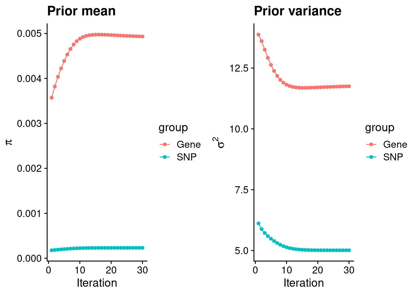

Version	Author	Date
3a7fbc1	wesleycrouse	2021-09-08

#estimated group prior
estimated_group_prior <- group_prior_rec[,ncol(group_prior_rec)]
names(estimated_group_prior) <- c("gene", "snp")
estimated_group_prior["snp"] <- estimated_group_prior["snp"]*thin #adjust parameter to account for thin argument
print(estimated_group_prior)

        gene          snp 
0.0049335272 0.0002320783

#estimated group prior variance
estimated_group_prior_var <- group_prior_var_rec[,ncol(group_prior_var_rec)]
names(estimated_group_prior_var) <- c("gene", "snp")
print(estimated_group_prior_var)

     gene       snp 
11.749699  5.009056

#report sample size
print(sample_size)

[1] 336473

#report group size
group_size <- c(nrow(ctwas_gene_res), n_snps)
print(group_size)

[1]   10290 7535010

#estimated group PVE
estimated_group_pve <- estimated_group_prior_var*estimated_group_prior*group_size/sample_size #check PVE calculation
names(estimated_group_pve) <- c("gene", "snp")
print(estimated_group_pve)

       gene         snp 
0.001772758 0.026032994

#compare sum(PIP*mu2/sample_size) with above PVE calculation
c(sum(ctwas_gene_res$PVE),sum(ctwas_snp_res$PVE))

[1] 0.007268092 0.373612404

Genes with highest PIPs

#distribution of PIPs
hist(ctwas_gene_res$susie_pip, xlim=c(0,1), main="Distribution of Gene PIPs")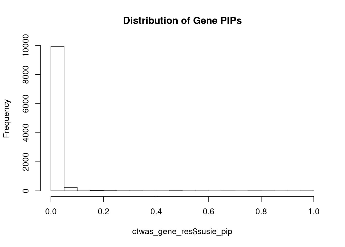

Version	Author	Date
3a7fbc1	wesleycrouse	2021-09-08

#genes with PIP>0.8 or 20 highest PIPs
head(ctwas_gene_res[order(-ctwas_gene_res$susie_pip),report_cols], max(sum(ctwas_gene_res$susie_pip>0.8), 20))

       genename region_tag susie_pip   mu2     PVE     z
3212      CCND2       12_4     0.999 94.77 2.8e-04  9.93
7394   TP53INP1       8_66     0.804 27.04 6.5e-05  4.85
1231     PABPC4       1_24     0.787 27.84 6.5e-05  5.08
9756   C17orf58      17_39     0.758 25.23 5.7e-05  4.46
7040      INHBB       2_70     0.751 23.97 5.3e-05 -4.22
1960     SNAPC2       19_7     0.699 26.22 5.4e-05 -4.44
6307       NUS1       6_78     0.660 23.46 4.6e-05  4.44
11990      BOP1       8_94     0.555 22.92 3.8e-05 -4.12
12661 LINC01126       2_27     0.533 43.82 6.9e-05  6.95
10049  GTF2IRD2       7_48     0.499 27.40 4.1e-05 -5.11
12035     GTF2I       7_48     0.499 27.40 4.1e-05 -5.11
10017     PTPRT      20_27     0.498 31.06 4.6e-05  3.88
11478   HLA-DMB       6_27     0.496 31.05 4.6e-05 -4.72
3475      ZMIZ2       7_33     0.483 23.24 3.3e-05  4.09
3091      RAB29      1_104     0.463 22.70 3.1e-05  4.01
6374      RAB6B       3_83     0.441 30.23 4.0e-05  3.88
1819       RBL2      16_29     0.357 25.78 2.7e-05 -4.91
9311     UBE2E2       3_17     0.313 25.74 2.4e-05 -4.52
9082     RAD23A      19_10     0.305 24.11 2.2e-05  4.10
6471      FGF18      5_102     0.302 40.95 3.7e-05  3.72

Genes with largest effect sizes

#plot PIP vs effect size
plot(ctwas_gene_res$susie_pip, ctwas_gene_res$mu2, xlab="PIP", ylab="mu^2", main="Gene PIPs vs Effect Size")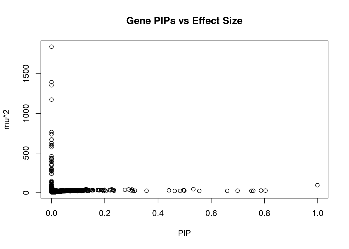

Version	Author	Date
3a7fbc1	wesleycrouse	2021-09-08

#genes with 20 largest effect sizes
head(ctwas_gene_res[order(-ctwas_gene_res$mu2),report_cols],20)

      genename region_tag susie_pip     mu2     PVE     z
10639     MICB       6_25         0 1840.96 0.0e+00 -8.27
11110      LTA       6_25         0 1392.74 0.0e+00 -5.83
10771    HCG27       6_25         0 1353.80 0.0e+00 -6.24
11366 HLA-DQA2       6_26         0 1173.79 0.0e+00 -9.63
3254     BBOF1      14_34         0  764.96 0.0e+00 -3.13
10599   NOTCH4       6_26         0  737.34 0.0e+00  6.67
10183  ZSCAN26       6_22         0  671.26 0.0e+00  3.78
10603   AGPAT1       6_26         0  668.45 0.0e+00 -5.74
11216  CYP21A2       6_26         0  627.35 0.0e+00 -8.87
10374  ZKSCAN8       6_22         0  600.02 0.0e+00 -2.68
6443   FAM161B      14_34         0  595.90 0.0e+00 -2.35
9792    ENTPD5      14_34         0  573.46 0.0e+00  2.24
10852 ATP6V1G2       6_25         0  459.30 0.0e+00 -2.63
3274      COQ6      14_34         0  434.82 0.0e+00 -1.89
10849    DDAH2       6_26         0  434.36 0.0e+00  7.99
10602     RNF5       6_26         0  431.20 0.0e+00  5.29
10339   MARCH5      10_59         0  426.10 7.9e-16  1.85
10597  HLA-DRA       6_26         0  416.43 0.0e+00  6.54
11541      C4A       6_26         0  394.05 0.0e+00  6.85
2263     CPEB3      10_59         0  390.36 6.6e-16 -1.85

Genes with highest PVE

#genes with 20 highest pve
head(ctwas_gene_res[order(-ctwas_gene_res$PVE),report_cols],20)

       genename region_tag susie_pip   mu2     PVE     z
3212      CCND2       12_4     0.999 94.77 2.8e-04  9.93
12661 LINC01126       2_27     0.533 43.82 6.9e-05  6.95
1231     PABPC4       1_24     0.787 27.84 6.5e-05  5.08
7394   TP53INP1       8_66     0.804 27.04 6.5e-05  4.85
9756   C17orf58      17_39     0.758 25.23 5.7e-05  4.46
1960     SNAPC2       19_7     0.699 26.22 5.4e-05 -4.44
7040      INHBB       2_70     0.751 23.97 5.3e-05 -4.22
6307       NUS1       6_78     0.660 23.46 4.6e-05  4.44
10017     PTPRT      20_27     0.498 31.06 4.6e-05  3.88
11478   HLA-DMB       6_27     0.496 31.05 4.6e-05 -4.72
10049  GTF2IRD2       7_48     0.499 27.40 4.1e-05 -5.11
12035     GTF2I       7_48     0.499 27.40 4.1e-05 -5.11
6374      RAB6B       3_83     0.441 30.23 4.0e-05  3.88
11990      BOP1       8_94     0.555 22.92 3.8e-05 -4.12
6471      FGF18      5_102     0.302 40.95 3.7e-05  3.72
9378     ZNF320      19_36     0.290 41.57 3.6e-05 -3.73
3475      ZMIZ2       7_33     0.483 23.24 3.3e-05  4.09
3091      RAB29      1_104     0.463 22.70 3.1e-05  4.01
6036     ARID5B      10_42     0.226 43.26 2.9e-05  3.71
9887    NCR3LG1      11_12     0.276 35.72 2.9e-05  5.87

Genes with largest z scores

#genes with 20 largest z scores
head(ctwas_gene_res[order(-abs(ctwas_gene_res$z)),report_cols],20)

       genename region_tag susie_pip     mu2     PVE     z
3212      CCND2       12_4     0.999   94.77 2.8e-04  9.93
11366  HLA-DQA2       6_26     0.000 1173.79 0.0e+00 -9.63
11216   CYP21A2       6_26     0.000  627.35 0.0e+00 -8.87
10639      MICB       6_25     0.000 1840.96 0.0e+00 -8.27
10849     DDAH2       6_26     0.000  434.36 0.0e+00  7.99
10594     PSMB8       6_27     0.003   47.65 3.6e-07 -7.14
12661 LINC01126       2_27     0.533   43.82 6.9e-05  6.95
11541       C4A       6_26     0.000  394.05 0.0e+00  6.85
10599    NOTCH4       6_26     0.000  737.34 0.0e+00  6.67
10848     CLIC1       6_26     0.000  359.42 0.0e+00  6.63
11415     PSMB9       6_27     0.005   46.57 6.9e-07 -6.63
10597   HLA-DRA       6_26     0.000  416.43 0.0e+00  6.54
10771     HCG27       6_25     0.000 1353.80 0.0e+00 -6.24
9887    NCR3LG1      11_12     0.276   35.72 2.9e-05  5.87
11110       LTA       6_25     0.000 1392.74 0.0e+00 -5.83
10603    AGPAT1       6_26     0.000  668.45 0.0e+00 -5.74
4833      FLOT1       6_24     0.179   30.41 1.6e-05 -5.38
6558      AP3S2      15_41     0.221   30.24 2.0e-05 -5.33
10602      RNF5       6_26     0.000  431.20 0.0e+00  5.29
2887      NRBP1       2_16     0.013   32.45 1.2e-06  5.22

Comparing z scores and PIPs

#set nominal signifiance threshold for z scores
alpha <- 0.05

#bonferroni adjusted threshold for z scores
sig_thresh <- qnorm(1-(alpha/nrow(ctwas_gene_res)/2), lower=T)

#Q-Q plot for z scores
obs_z <- ctwas_gene_res$z[order(ctwas_gene_res$z)]
exp_z <- qnorm((1:nrow(ctwas_gene_res))/nrow(ctwas_gene_res))

plot(exp_z, obs_z, xlab="Expected z", ylab="Observed z", main="Gene z score Q-Q plot")
abline(a=0,b=1)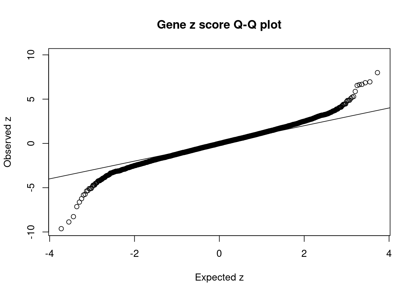

Version	Author	Date
3a7fbc1	wesleycrouse	2021-09-08

#plot z score vs PIP
plot(abs(ctwas_gene_res$z), ctwas_gene_res$susie_pip, xlab="abs(z)", ylab="PIP")
abline(v=sig_thresh, col="red", lty=2)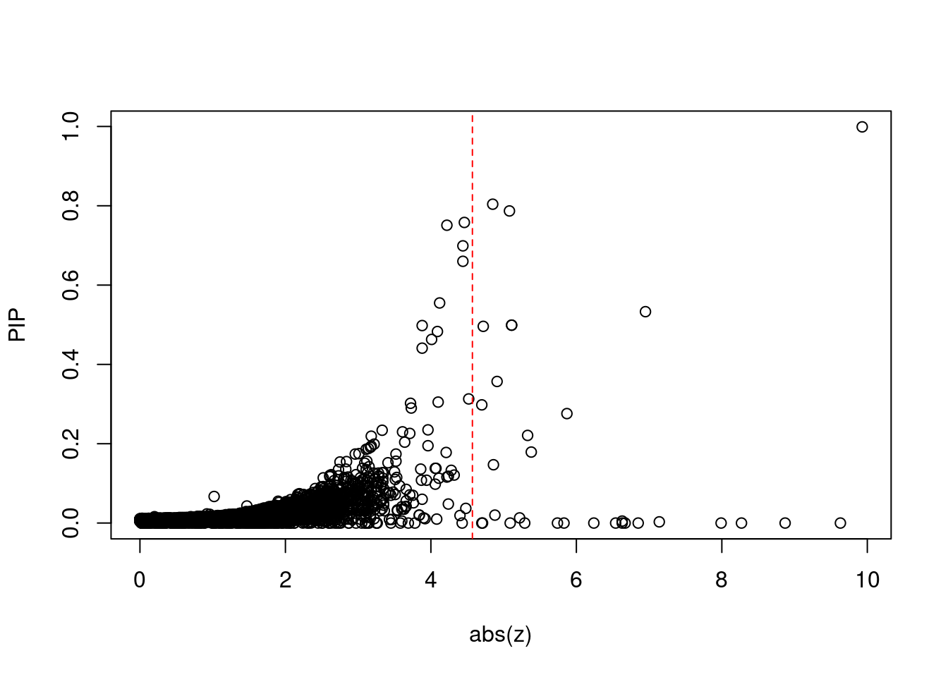

Version	Author	Date
3a7fbc1	wesleycrouse	2021-09-08

#proportion of significant z scores
mean(abs(ctwas_gene_res$z) > sig_thresh)

[1] 0.003109815

#genes with most significant z scores
head(ctwas_gene_res[order(-abs(ctwas_gene_res$z)),report_cols],20)

       genename region_tag susie_pip     mu2     PVE     z
3212      CCND2       12_4     0.999   94.77 2.8e-04  9.93
11366  HLA-DQA2       6_26     0.000 1173.79 0.0e+00 -9.63
11216   CYP21A2       6_26     0.000  627.35 0.0e+00 -8.87
10639      MICB       6_25     0.000 1840.96 0.0e+00 -8.27
10849     DDAH2       6_26     0.000  434.36 0.0e+00  7.99
10594     PSMB8       6_27     0.003   47.65 3.6e-07 -7.14
12661 LINC01126       2_27     0.533   43.82 6.9e-05  6.95
11541       C4A       6_26     0.000  394.05 0.0e+00  6.85
10599    NOTCH4       6_26     0.000  737.34 0.0e+00  6.67
10848     CLIC1       6_26     0.000  359.42 0.0e+00  6.63
11415     PSMB9       6_27     0.005   46.57 6.9e-07 -6.63
10597   HLA-DRA       6_26     0.000  416.43 0.0e+00  6.54
10771     HCG27       6_25     0.000 1353.80 0.0e+00 -6.24
9887    NCR3LG1      11_12     0.276   35.72 2.9e-05  5.87
11110       LTA       6_25     0.000 1392.74 0.0e+00 -5.83
10603    AGPAT1       6_26     0.000  668.45 0.0e+00 -5.74
4833      FLOT1       6_24     0.179   30.41 1.6e-05 -5.38
6558      AP3S2      15_41     0.221   30.24 2.0e-05 -5.33
10602      RNF5       6_26     0.000  431.20 0.0e+00  5.29
2887      NRBP1       2_16     0.013   32.45 1.2e-06  5.22

Locus plots for genes and SNPs

ctwas_gene_res_sortz <- ctwas_gene_res[order(-abs(ctwas_gene_res$z)),]

n_plots <- 5
for (region_tag_plot in head(unique(ctwas_gene_res_sortz$region_tag), n_plots)){
  ctwas_res_region <-  ctwas_res[ctwas_res$region_tag==region_tag_plot,]
  start <- min(ctwas_res_region$pos)
  end <- max(ctwas_res_region$pos)
  
  ctwas_res_region <- ctwas_res_region[order(ctwas_res_region$pos),]
  ctwas_res_region_gene <- ctwas_res_region[ctwas_res_region$type=="gene",]
  ctwas_res_region_snp <- ctwas_res_region[ctwas_res_region$type=="SNP",]
  
  #region name
  print(paste0("Region: ", region_tag_plot))
  
  #table of genes in region
  print(ctwas_res_region_gene[,report_cols])
  
  par(mfrow=c(4,1))
  
  #gene z scores
  plot(ctwas_res_region_gene$pos, abs(ctwas_res_region_gene$z), xlab="Position", ylab="abs(gene_z)", xlim=c(start,end),
   ylim=c(0,max(sig_thresh, abs(ctwas_res_region_gene$z))),
   main=paste0("Region: ", region_tag_plot))
  abline(h=sig_thresh,col="red",lty=2)
  
  #significance threshold for SNPs
  alpha_snp <- 5*10^(-8)
  sig_thresh_snp <- qnorm(1-alpha_snp/2, lower=T)
  
  #snp z scores
  plot(ctwas_res_region_snp$pos, abs(ctwas_res_region_snp$z), xlab="Position", ylab="abs(snp_z)",xlim=c(start,end),
   ylim=c(0,max(sig_thresh_snp, max(abs(ctwas_res_region_snp$z)))))
  abline(h=sig_thresh_snp,col="purple",lty=2)
  
  #gene pips
  plot(ctwas_res_region_gene$pos, ctwas_res_region_gene$susie_pip, xlab="Position", ylab="Gene PIP", xlim=c(start,end), ylim=c(0,1))
  abline(h=0.8,col="blue",lty=2)
  
  #snp pips
  plot(ctwas_res_region_snp$pos, ctwas_res_region_snp$susie_pip, xlab="Position", ylab="SNP PIP", xlim=c(start,end), ylim=c(0,1))
  abline(h=0.8,col="blue",lty=2)
}

[1] "Region: 12_4"
          genename region_tag susie_pip   mu2     PVE     z
4041       CRACR2A       12_4     0.011 15.06 5.1e-07 -1.64
2530        PARP11       12_4     0.018 19.64 1.1e-06 -2.06
11823 RP11-320N7.2       12_4     0.008 12.39 3.0e-07 -1.44
3212         CCND2       12_4     0.999 94.77 2.8e-04  9.93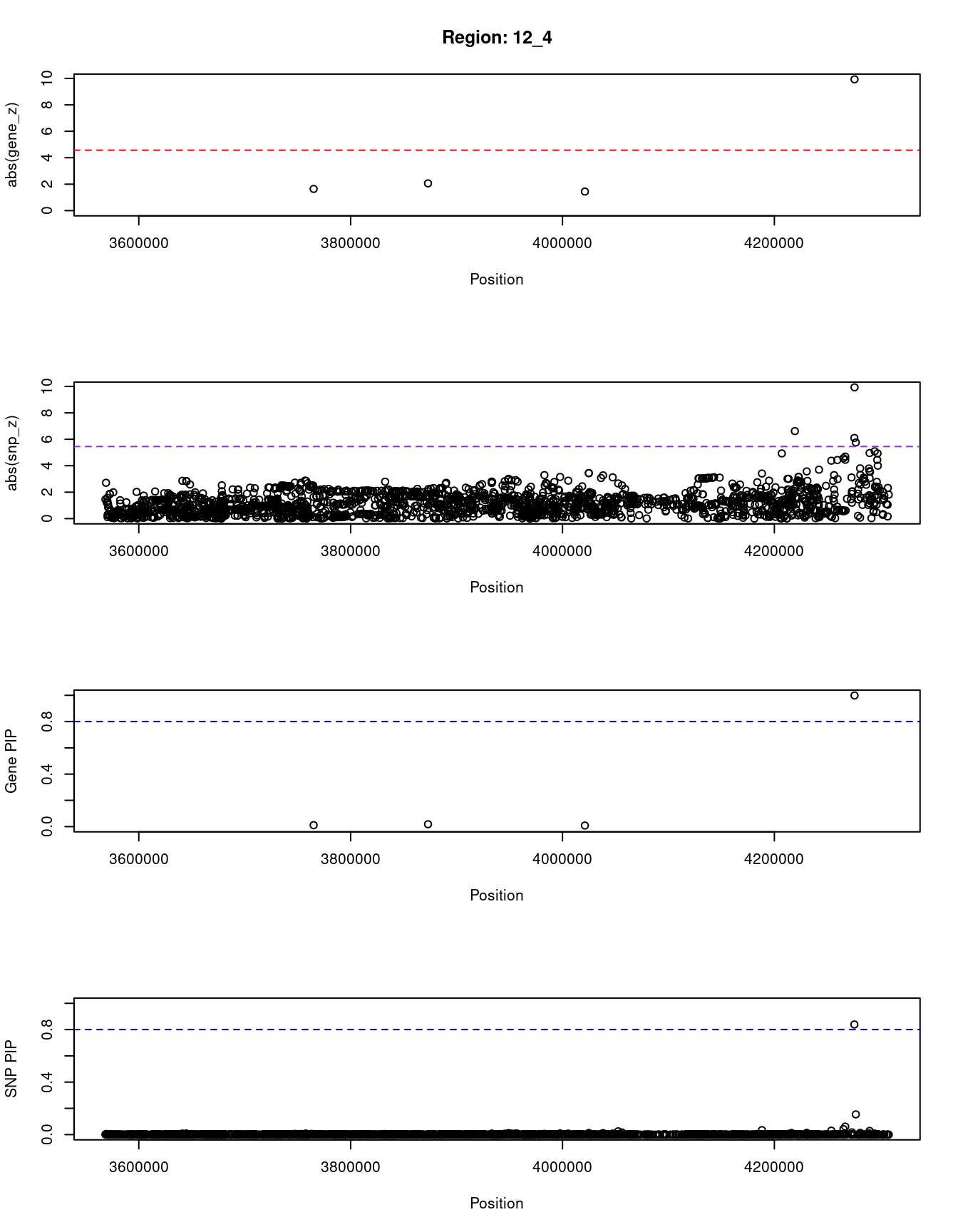

Version	Author	Date
3a7fbc1	wesleycrouse	2021-09-08

[1] "Region: 6_26"
      genename region_tag susie_pip     mu2 PVE     z
10632     BAG6       6_26         0    7.98   0  0.76
10634     AIF1       6_26         0    5.33   0 -0.25
10633   PRRC2A       6_26         0   45.41   0 -3.25
10631     APOM       6_26         0   29.25   0 -1.88
10630  C6orf47       6_26         0   31.60   0 -1.95
10629   CSNK2B       6_26         0   70.66   0  1.03
11414   LY6G5B       6_26         0   29.26   0  0.14
10627  ABHD16A       6_26         0   53.03   0  2.87
10626   MPIG6B       6_26         0   18.61   0  0.82
10849    DDAH2       6_26         0  434.36   0  7.99
10625     MSH5       6_26         0  122.20   0  4.43
10848    CLIC1       6_26         0  359.42   0  6.63
10623     VWA7       6_26         0   39.12   0  2.30
10622     LSM2       6_26         0   23.59   0 -0.53
10621   HSPA1L       6_26         0   12.33   0  0.78
10619  C6orf48       6_26         0   15.35   0  0.03
10618  SLC44A4       6_26         0   77.12   0 -3.69
10616    EHMT2       6_26         0   59.18   0  1.23
10612   SKIV2L       6_26         0   12.22   0  1.11
10610    STK19       6_26         0   41.00   0  1.64
10611      DXO       6_26         0   82.57   0 -3.45
11541      C4A       6_26         0  394.05   0  6.85
11216  CYP21A2       6_26         0  627.35   0 -8.87
11038      C4B       6_26         0   86.96   0  1.12
10844    ATF6B       6_26         0   55.93   0 -2.60
7949      TNXB       6_26         0   50.26   0  2.87
10606    FKBPL       6_26         0  130.25   0 -0.27
11007     PPT2       6_26         0  273.88   0 -3.15
10605    PRRT1       6_26         0   24.56   0  0.14
11441    EGFL8       6_26         0   14.78   0 -1.62
10603   AGPAT1       6_26         0  668.45   0 -5.74
10601     AGER       6_26         0   11.90   0  2.01
10602     RNF5       6_26         0  431.20   0  5.29
10600     PBX2       6_26         0   36.76   0  0.25
10599   NOTCH4       6_26         0  737.34   0  6.67
10597  HLA-DRA       6_26         0  416.43   0  6.54
10137 HLA-DQA1       6_26         0  293.97   0  0.57
11366 HLA-DQA2       6_26         0 1173.79   0 -9.63

Version	Author	Date
3a7fbc1	wesleycrouse	2021-09-08

[1] "Region: 6_25"
               genename region_tag susie_pip     mu2 PVE     z
10653              DDR1       6_25         0  101.67   0  3.58
4838              VARS2       6_25         0   79.72   0  3.26
10854            GTF2H4       6_25         0   99.70   0  4.71
10044             SFTA2       6_25         0    5.86   0  0.53
10646          PSORS1C1       6_25         0  232.96   0 -0.51
10645          PSORS1C2       6_25         0  302.73   0 -3.05
11297             HLA-B       6_25         0  140.64   0 -4.70
4832              TCF19       6_25         0   28.31   0 -1.68
10644            CCHCR1       6_25         0   28.31   0 -1.68
10643            POU5F1       6_25         0  352.21   0 -5.09
10771             HCG27       6_25         0 1353.80   0 -6.24
10642             HLA-C       6_25         0  289.58   0  1.55
12306 XXbac-BPG181B23.7       6_25         0  302.30   0  2.74
10640              MICA       6_25         0  104.93   0 -3.10
10639              MICB       6_25         0 1840.96   0 -8.27
10417            DDX39B       6_25         0   66.61   0 -1.76
10637           NFKBIL1       6_25         0  242.65   0  0.59
10852          ATP6V1G2       6_25         0  459.30   0 -2.63
11110               LTA       6_25         0 1392.74   0 -5.83
11237               TNF       6_25         0   40.67   0  2.12
10635              NCR3       6_25         0   86.68   0  3.26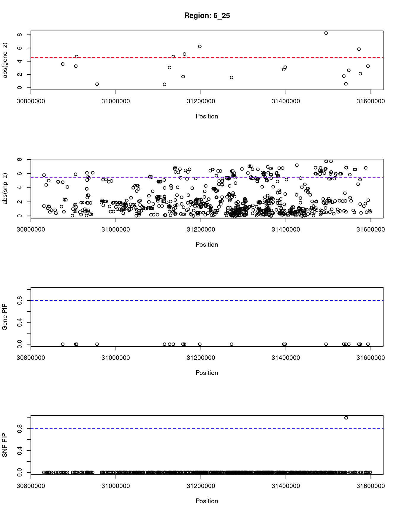

Version	Author	Date
3a7fbc1	wesleycrouse	2021-09-08

[1] "Region: 6_27"
      genename region_tag susie_pip   mu2     PVE     z
11435  HLA-DOB       6_27     0.000 30.43 1.9e-08 -2.32
10595     TAP2       6_27     0.000 26.07 2.1e-08  1.41
11415    PSMB9       6_27     0.005 46.57 6.9e-07 -6.63
10594    PSMB8       6_27     0.003 47.65 3.6e-07 -7.14
7936      TAP1       6_27     0.000 11.40 1.1e-08 -2.50
11478  HLA-DMB       6_27     0.496 31.05 4.6e-05 -4.72
10591  HLA-DMA       6_27     0.013 19.51 7.6e-07 -3.90
10590     BRD2       6_27     0.000  6.61 4.7e-09  3.10
10589  HLA-DOA       6_27     0.002 11.78 6.3e-08 -0.73
10588  COL11A2       6_27     0.001 15.18 5.7e-08  2.01
10586     RXRB       6_27     0.000  6.46 5.0e-09  0.22
10585  HSD17B8       6_27     0.000  9.64 7.7e-09 -1.46
10584    RING1       6_27     0.000  6.62 5.2e-09 -0.25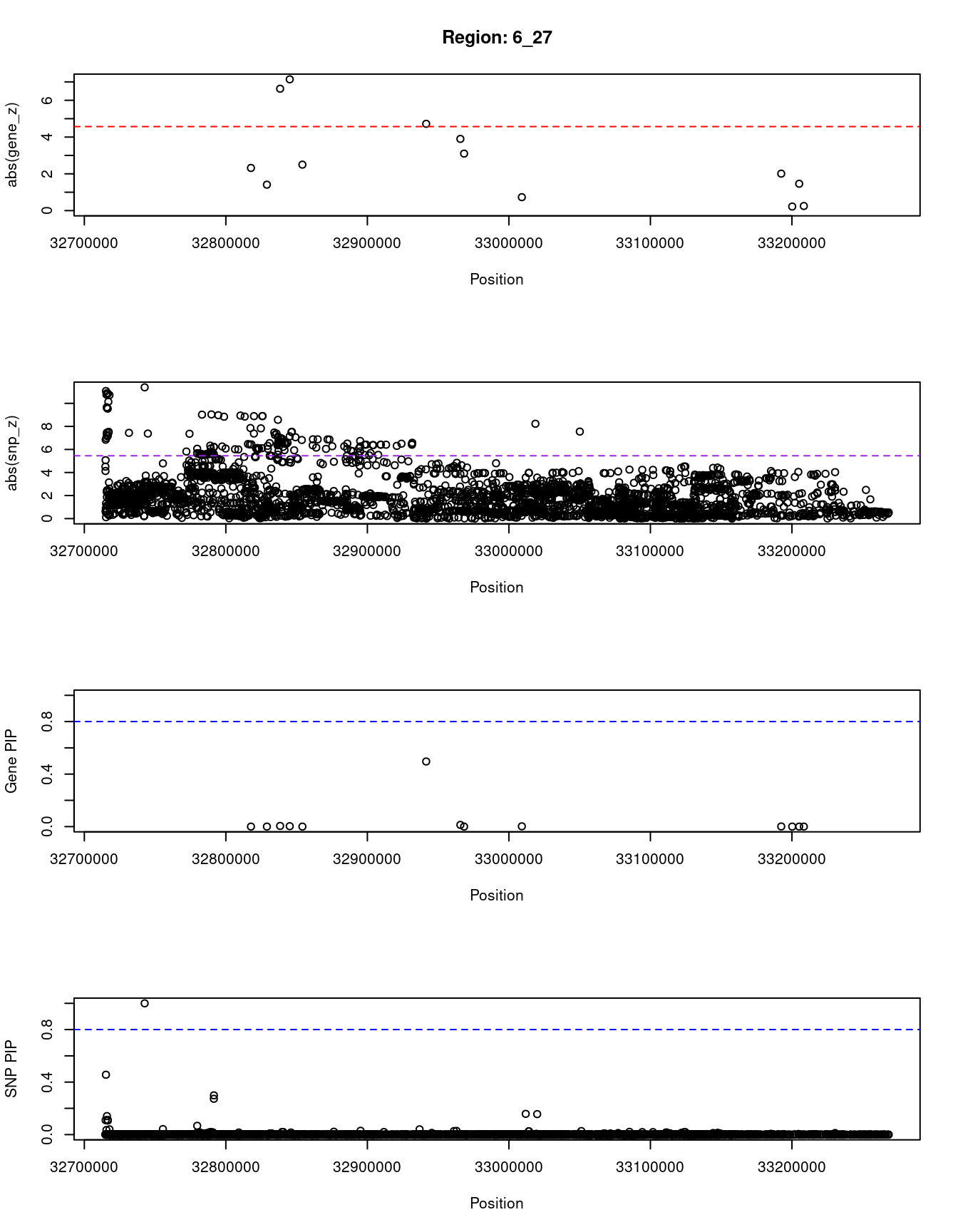

Version	Author	Date
3a7fbc1	wesleycrouse	2021-09-08

[1] "Region: 2_27"
        genename region_tag susie_pip   mu2     PVE     z
12661  LINC01126       2_27     0.533 43.82 6.9e-05  6.95
2977       THADA       2_27     0.008  5.36 1.2e-07  0.98
6208     PLEKHH2       2_27     0.008  4.67 1.1e-07 -0.30
11022 C1GALT1C1L       2_27     0.008  5.09 1.2e-07 -0.70
4930    DYNC2LI1       2_27     0.024 15.73 1.1e-06  1.90
5563       ABCG8       2_27     0.008  5.08 1.2e-07 -0.05
4943      LRPPRC       2_27     0.008  5.56 1.4e-07  0.61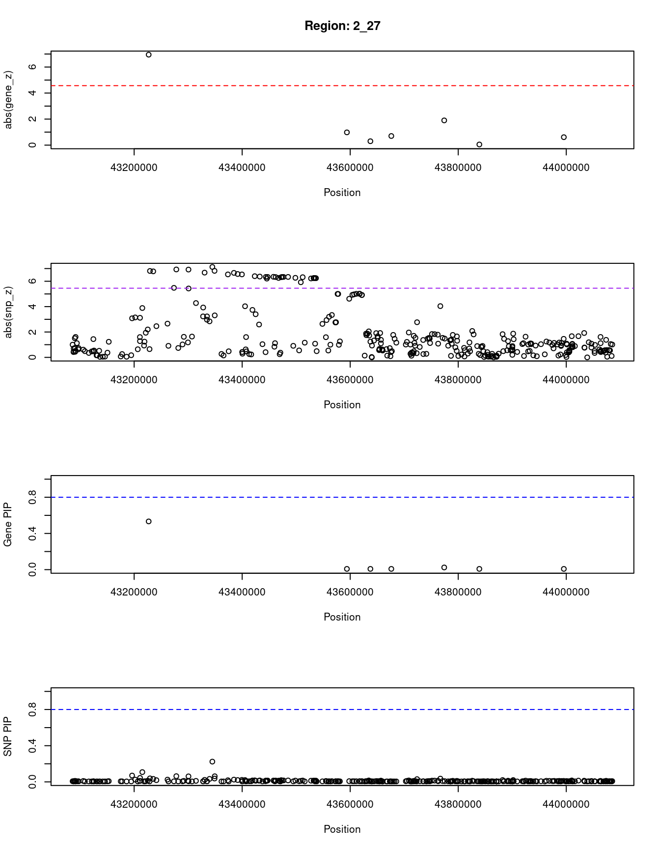

Version	Author	Date
3a7fbc1	wesleycrouse	2021-09-08

SNPs with highest PIPs

#snps with PIP>0.8 or 20 highest PIPs
head(ctwas_snp_res[order(-ctwas_snp_res$susie_pip),report_cols_snps],
max(sum(ctwas_snp_res$susie_pip>0.8), 20))

                id region_tag susie_pip     mu2     PVE     z
37018   rs75222047       1_85     1.000  680.34 2.0e-03  2.91
82161   rs12471681       2_53     1.000  782.94 2.3e-03 -3.05
140714  rs13062973       3_45     1.000  541.31 1.6e-03 -3.60
168715   rs1388475      3_107     1.000  444.24 1.3e-03  2.87
168716  rs13071192      3_107     1.000  423.68 1.3e-03 -3.12
171181  rs28661518      3_112     1.000  822.04 2.4e-03 -3.09
210999   rs2125449       4_79     1.000  855.29 2.5e-03 -3.33
254120   rs3910018       5_51     1.000  697.79 2.1e-03 -2.86
285519   rs2206734       6_15     1.000   82.45 2.5e-04 10.34
287817  rs34662244       6_22     1.000 1460.04 4.3e-03  4.07
287835  rs67297533       6_22     1.000 1424.70 4.2e-03 -4.09
289917   rs2523507       6_25     1.000 4018.24 1.2e-02  6.84
289918   rs2239528       6_25     1.000 4117.93 1.2e-02 -6.84
290443   rs9272679       6_26     1.000 1599.33 4.8e-03 -9.31
290452  rs17612548       6_26     1.000 1677.37 5.0e-03 11.17
290473   rs3134996       6_26     1.000 1652.70 4.9e-03 10.37
381892   rs1495743       8_20     1.000  367.53 1.1e-03  3.21
409376  rs16902104       8_83     1.000 1073.73 3.2e-03  3.51
438249   rs7025746       9_53     1.000  335.79 1.0e-03 -3.04
438253   rs2900388       9_53     1.000  329.59 9.8e-04  3.51
473660   rs2019640      10_59     1.000  864.21 2.6e-03 -3.47
473662    rs913647      10_59     1.000  866.71 2.6e-03  3.45
479015  rs12244851      10_70     1.000  252.90 7.5e-04 22.39
486553    rs234856       11_2     1.000   36.40 1.1e-04 -4.94
488586  rs11041828       11_6     1.000  746.13 2.2e-03  2.96
488587   rs4237770       11_6     1.000  764.34 2.3e-03 -2.93
500526 rs113527193      11_30     1.000  421.22 1.3e-03  3.29
500857  rs11603701      11_30     1.000  403.70 1.2e-03 -3.24
614809  rs12912777      15_13     1.000   32.59 9.7e-05  5.53
651300  rs12443634      16_45     1.000  177.55 5.3e-04 -3.47
651307   rs2966092      16_45     1.000  179.96 5.3e-04  3.38
656828   rs4790233       17_5     1.000  187.16 5.6e-04 -3.70
656833   rs8072531       17_5     1.000  187.97 5.6e-04 -3.98
702485  rs73537429      19_15     1.000  239.17 7.1e-04 -2.52
721881   rs2747568      20_20     1.000 1125.55 3.3e-03  3.79
721882   rs2064505      20_20     1.000 1156.77 3.4e-03 -3.92
751689 rs115018313       6_27     1.000   63.01 1.9e-04 11.39
770312  rs72627126      14_34     1.000  979.66 2.9e-03 -3.38
65949     rs780093       2_16     0.999   41.48 1.2e-04  6.98
431567   rs9410573       9_40     0.999   46.51 1.4e-04 -7.44
663718   rs9906451      17_22     0.999   30.16 9.0e-05 -5.87
702514   rs2285626      19_15     0.997  106.58 3.2e-04  5.36
576175   rs1327315      13_40     0.994   32.42 9.6e-05 -7.40
422855  rs10965243       9_16     0.990   26.19 7.7e-05 -5.41
381895  rs34537991       8_20     0.988  317.51 9.3e-04  3.06
47621   rs79687284      1_108     0.974   25.18 7.3e-05  5.66
438252   rs7868850       9_53     0.972   62.68 1.8e-04  0.83
702487  rs67238925      19_15     0.969  230.22 6.6e-04  2.39
438250   rs4742930       9_53     0.964  261.33 7.5e-04  3.25
168718  rs13081434      3_107     0.951  405.57 1.1e-03 -2.47
29222    rs6679677       1_70     0.945   25.75 7.2e-05  5.33
486552    rs234852       11_2     0.940   25.35 7.1e-05  3.12
539824    rs189339      12_40     0.938   32.90 9.2e-05 -6.27
409375  rs16902103       8_83     0.933 1047.87 2.9e-03 -3.50
155021  rs72964564       3_76     0.930   32.77 9.1e-05 -6.10
473740   rs1977833      10_59     0.925   93.94 2.6e-04 -8.47
171182  rs73190822      3_112     0.917  801.56 2.2e-03  3.11
257315  rs10479168       5_59     0.908   25.96 7.0e-05  5.36
576187    rs502027      13_40     0.907   31.44 8.5e-05  7.22
172066   rs6444187      3_114     0.899   25.43 6.8e-05  5.17
536873   rs2682323      12_33     0.876   23.91 6.2e-05  4.74
648543  rs72802395      16_40     0.869   35.23 9.1e-05 -6.35
205552  rs35518360       4_67     0.867   24.30 6.3e-05  4.70
47625     rs340835      1_108     0.849   25.60 6.5e-05  5.52
762856   rs3217792       12_4     0.839   36.67 9.1e-05 -6.10
139980   rs3774723       3_43     0.825   24.62 6.0e-05 -4.84
609711 rs117618513      14_54     0.824   25.06 6.1e-05 -4.96
171180  rs62287225      3_112     0.821  801.31 2.0e-03  3.08
664773    rs665268      17_25     0.818   26.19 6.4e-05  5.36
607280  rs11160254      14_49     0.816   23.94 5.8e-05  4.55
140702  rs34695932       3_45     0.814  568.02 1.4e-03  4.13
656824  rs79425343       17_5     0.813   23.29 5.6e-05  1.15
160561  rs73148854       3_89     0.812   23.00 5.6e-05 -4.35
37037    rs2179109       1_85     0.802  664.66 1.6e-03 -3.03
709542  rs12609461      19_33     0.801   28.71 6.8e-05  5.53

SNPs with largest effect sizes

#plot PIP vs effect size
plot(ctwas_snp_res$susie_pip, ctwas_snp_res$mu2, xlab="PIP", ylab="mu^2", main="SNP PIPs vs Effect Size")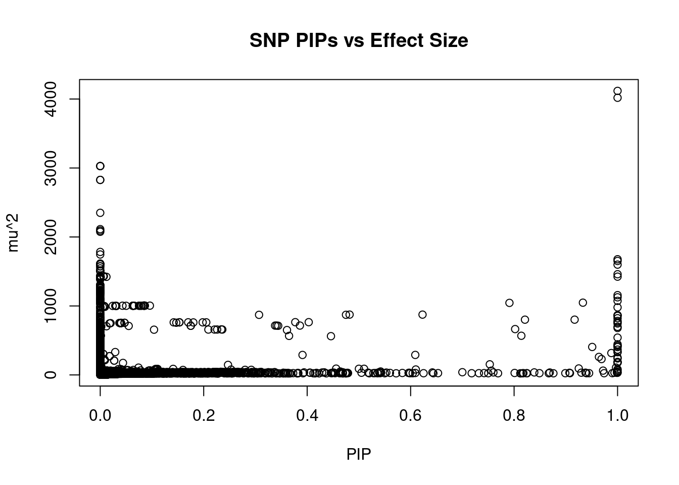

Version	Author	Date
3a7fbc1	wesleycrouse	2021-09-08

#SNPs with 50 largest effect sizes
head(ctwas_snp_res[order(-ctwas_snp_res$mu2),report_cols_snps],50)

               id region_tag susie_pip     mu2     PVE     z
289918  rs2239528       6_25     1.000 4117.93 1.2e-02 -6.84
289917  rs2523507       6_25     1.000 4018.24 1.2e-02  6.84
289897  rs3093953       6_25     0.000 3028.17 0.0e+00  6.20
289894  rs2286713       6_25     0.000 3028.15 0.0e+00  6.20
289896  rs3093954       6_25     0.000 3028.15 0.0e+00  6.20
289911  rs3093979       6_25     0.000 2827.51 0.0e+00  5.97
289910  rs3093984       6_25     0.000 2827.33 0.0e+00  5.97
289876  rs9267293       6_25     0.000 2350.43 0.0e+00  6.07
289866  rs2905722       6_25     0.000 2113.61 0.0e+00  6.81
289856  rs2523670       6_25     0.000 2092.64 0.0e+00  6.83
289904  rs3094000       6_25     0.000 2075.37 0.0e+00  5.76
289893 rs28703977       6_25     0.000 1783.38 0.0e+00  5.94
289807  rs3132091       6_25     0.000 1746.43 0.0e+00  7.19
290452 rs17612548       6_26     1.000 1677.37 5.0e-03 11.17
290473  rs3134996       6_26     1.000 1652.70 4.9e-03 10.37
290451 rs17612510       6_26     0.000 1615.60 1.8e-08 10.42
290459  rs9273524       6_26     0.000 1608.00 0.0e+00 10.93
289924  rs2516391       6_25     0.000 1607.63 0.0e+00  6.59
289925  rs3094595       6_25     0.000 1607.57 0.0e+00  6.58
289926   rs928815       6_25     0.000 1606.98 0.0e+00  6.58
290453 rs17612633       6_26     0.000 1606.90 0.0e+00 10.90
290450  rs9273242       6_26     0.000 1602.81 0.0e+00 10.58
290443  rs9272679       6_26     1.000 1599.33 4.8e-03 -9.31
289441  rs9264024       6_25     0.000 1576.14 0.0e+00  6.59
289440  rs3130520       6_25     0.000 1573.19 0.0e+00  6.56
289691  rs2596488       6_25     0.000 1544.49 0.0e+00  6.95
289509  rs3134744       6_25     0.000 1512.94 0.0e+00  6.36
289502 rs28498059       6_25     0.000 1512.18 0.0e+00  6.35
289459  rs3130532       6_25     0.000 1508.55 0.0e+00  6.37
289464  rs3095246       6_25     0.000 1508.29 0.0e+00  6.36
289431  rs3130950       6_25     0.000 1505.84 0.0e+00  6.41
287817 rs34662244       6_22     1.000 1460.04 4.3e-03  4.07
289688  rs2523605       6_25     0.000 1440.50 0.0e+00  4.99
287872 rs13191786       6_22     0.007 1431.46 2.8e-05  4.10
287875 rs34218844       6_22     0.006 1431.22 2.4e-05  4.09
289887  rs2855807       6_25     0.000 1428.45 0.0e+00  5.27
289891  rs2534659       6_25     0.000 1428.44 0.0e+00  5.27
289657  rs2508000       6_25     0.000 1428.13 0.0e+00  5.98
287835 rs67297533       6_22     1.000 1424.70 4.2e-03 -4.09
287861 rs67998226       6_22     0.012 1422.40 5.3e-05  4.25
287880 rs35030260       6_22     0.001 1420.52 4.1e-06  4.12
287866 rs33932084       6_22     0.000 1415.33 5.3e-08  3.93
287885 rs13198809       6_22     0.000 1396.66 1.1e-08  4.08
289607  rs9264970       6_25     0.000 1395.03 0.0e+00  6.08
287894 rs36092177       6_22     0.000 1390.25 2.4e-09  4.08
287919 rs55690788       6_22     0.000 1383.81 2.3e-09  4.16
288031  rs1311917       6_22     0.000 1308.43 4.3e-19  3.82
288023  rs1233611       6_22     0.000 1307.38 0.0e+00  3.78
288041  rs9257192       6_22     0.000 1300.55 4.3e-19  3.92
288055  rs3135297       6_22     0.000 1299.88 4.3e-19  3.93

SNPs with highest PVE

#SNPs with 50 highest pve
head(ctwas_snp_res[order(-ctwas_snp_res$PVE),report_cols_snps],50)

                id region_tag susie_pip     mu2     PVE     z
289917   rs2523507       6_25     1.000 4018.24 0.01200  6.84
289918   rs2239528       6_25     1.000 4117.93 0.01200 -6.84
290452  rs17612548       6_26     1.000 1677.37 0.00500 11.17
290473   rs3134996       6_26     1.000 1652.70 0.00490 10.37
290443   rs9272679       6_26     1.000 1599.33 0.00480 -9.31
287817  rs34662244       6_22     1.000 1460.04 0.00430  4.07
287835  rs67297533       6_22     1.000 1424.70 0.00420 -4.09
721882   rs2064505      20_20     1.000 1156.77 0.00340 -3.92
721881   rs2747568      20_20     1.000 1125.55 0.00330  3.79
409376  rs16902104       8_83     1.000 1073.73 0.00320  3.51
409375  rs16902103       8_83     0.933 1047.87 0.00290 -3.50
770312  rs72627126      14_34     1.000  979.66 0.00290 -3.38
473660   rs2019640      10_59     1.000  864.21 0.00260 -3.47
473662    rs913647      10_59     1.000  866.71 0.00260  3.45
210999   rs2125449       4_79     1.000  855.29 0.00250 -3.33
409373  rs34585331       8_83     0.791 1044.69 0.00250 -3.55
171181  rs28661518      3_112     1.000  822.04 0.00240 -3.09
82161   rs12471681       2_53     1.000  782.94 0.00230 -3.05
488587   rs4237770       11_6     1.000  764.34 0.00230 -2.93
171182  rs73190822      3_112     0.917  801.56 0.00220  3.11
488586  rs11041828       11_6     1.000  746.13 0.00220  2.96
254120   rs3910018       5_51     1.000  697.79 0.00210 -2.86
37018   rs75222047       1_85     1.000  680.34 0.00200  2.91
171180  rs62287225      3_112     0.821  801.31 0.00200  3.08
37037    rs2179109       1_85     0.802  664.66 0.00160 -3.03
140714  rs13062973       3_45     1.000  541.31 0.00160 -3.60
211019  rs11721784       4_79     0.623  874.56 0.00160  3.38
140702  rs34695932       3_45     0.814  568.02 0.00140  4.13
168715   rs1388475      3_107     1.000  444.24 0.00130  2.87
168716  rs13071192      3_107     1.000  423.68 0.00130 -3.12
211006   rs1542437       4_79     0.482  874.77 0.00130  3.35
500526 rs113527193      11_30     1.000  421.22 0.00130  3.29
210985  rs13109930       4_79     0.475  872.03 0.00120  3.11
500857  rs11603701      11_30     1.000  403.70 0.00120 -3.24
168718  rs13081434      3_107     0.951  405.57 0.00110 -2.47
381892   rs1495743       8_20     1.000  367.53 0.00110  3.21
438249   rs7025746       9_53     1.000  335.79 0.00100 -3.04
438253   rs2900388       9_53     1.000  329.59 0.00098  3.51
381895  rs34537991       8_20     0.988  317.51 0.00093  3.06
82157   rs75755471       2_53     0.403  765.06 0.00092  3.07
82163   rs78406274       2_53     0.377  764.94 0.00086  3.06
254131  rs10805847       5_51     0.386  715.66 0.00082  2.87
210987   rs6819187       4_79     0.307  871.35 0.00080  3.09
140708  rs13071831       3_45     0.446  562.04 0.00075  4.15
438250   rs4742930       9_53     0.964  261.33 0.00075  3.25
479015  rs12244851      10_70     1.000  252.90 0.00075 22.39
254107  rs10064286       5_51     0.344  712.94 0.00073 -2.93
254125   rs3910025       5_51     0.341  715.49 0.00072  2.86
254126   rs3902731       5_51     0.338  715.48 0.00072  2.86
702485  rs73537429      19_15     1.000  239.17 0.00071 -2.52

SNPs with largest z scores

#SNPs with 50 largest z scores
head(ctwas_snp_res[order(-abs(ctwas_snp_res$z)),report_cols_snps],50)

                id region_tag susie_pip     mu2     PVE     z
479023  rs12260037      10_70     0.008  226.60 5.2e-06 22.65
479015  rs12244851      10_70     1.000  252.90 7.5e-04 22.39
479012   rs6585198      10_70     0.002  125.60 5.8e-07 15.56
479024  rs12359102      10_70     0.001   95.73 2.1e-07 14.81
479022   rs7077039      10_70     0.001   95.47 2.1e-07 14.79
479020   rs7921525      10_70     0.001   92.15 2.1e-07 14.58
479028   rs4077527      10_70     0.001   86.78 2.0e-07 14.57
479021   rs6585203      10_70     0.001   91.23 2.1e-07 14.52
479017  rs11196191      10_70     0.001   91.05 2.1e-07 14.51
479018  rs10787472      10_70     0.001   90.62 2.1e-07 14.49
290495   rs9275221       6_26     0.000  347.92 0.0e+00 12.84
290546   rs9275583       6_26     0.000  348.02 0.0e+00 12.83
290503   rs9275275       6_26     0.000  346.50 0.0e+00 12.82
290508   rs9275307       6_26     0.000  346.79 0.0e+00 12.82
290539   rs4273728       6_26     0.000  346.85 0.0e+00 12.82
290497   rs9275223       6_26     0.000  346.32 0.0e+00 12.81
290454  rs17612712       6_26     0.000 1163.31 0.0e+00 12.39
479006  rs12243578      10_70     0.003   79.99 7.1e-07 12.36
290515   rs9275362       6_26     0.000  180.03 0.0e+00 11.83
290456   rs9273354       6_26     0.000 1091.39 0.0e+00 11.78
751689 rs115018313       6_27     1.000   63.01 1.9e-04 11.39
290452  rs17612548       6_26     1.000 1677.37 5.0e-03 11.17
290375    rs617578       6_26     0.000  254.33 0.0e+00 11.10
751196   rs3873448       6_27     0.456   91.56 1.2e-04 11.07
290459   rs9273524       6_26     0.000 1608.00 0.0e+00 10.93
290453  rs17612633       6_26     0.000 1606.90 0.0e+00 10.90
751210   rs9275611       6_27     0.141   87.96 3.7e-05 10.89
751215   rs9275614       6_27     0.111   87.17 2.9e-05 10.84
751216   rs9275615       6_27     0.110   87.14 2.8e-05 10.84
751219   rs9275618       6_27     0.107   87.07 2.8e-05 10.84
290471   rs3828800       6_26     0.000  263.42 0.0e+00 10.83
751200   rs3873453       6_27     0.035   84.64 8.9e-06 10.76
290460   rs9273528       6_26     0.000  231.08 0.0e+00 10.73
751236   rs3916765       6_27     0.040   84.39 1.0e-05 10.72
290444  rs34763586       6_26     0.000  428.45 0.0e+00 10.63
290462  rs28724252       6_26     0.000  228.03 0.0e+00 10.61
290450   rs9273242       6_26     0.000 1602.81 0.0e+00 10.58
290363   rs2760985       6_26     0.000  403.41 0.0e+00 10.56
171760  rs11929397      3_114     0.510   89.57 1.4e-04 10.55
171761  rs11716713      3_114     0.500   89.51 1.3e-04 10.55
290369   rs2647066       6_26     0.000  402.89 0.0e+00 10.52
290518   rs3135002       6_26     0.000  974.09 0.0e+00 10.51
290388   rs3997872       6_26     0.000  403.70 0.0e+00 10.48
290451  rs17612510       6_26     0.000 1615.60 1.8e-08 10.42
290455  rs17612852       6_26     0.000 1173.94 0.0e+00 10.40
290473   rs3134996       6_26     1.000 1652.70 4.9e-03 10.37
285519   rs2206734       6_15     1.000   82.45 2.5e-04 10.34
290474   rs3134994       6_26     0.000 1075.68 0.0e+00 10.28
290468   rs3830058       6_26     0.000 1067.48 0.0e+00 10.17
751221   rs9275638       6_27     0.000   73.04 7.4e-08 10.14

Gene set enrichment for genes with PIP>0.8

#GO enrichment analysis
library(enrichR)

Welcome to enrichR
Checking connection ...

Enrichr ... Connection is Live!
FlyEnrichr ... Connection is available!
WormEnrichr ... Connection is available!
YeastEnrichr ... Connection is available!
FishEnrichr ... Connection is available!

dbs <- c("GO_Biological_Process_2021", "GO_Cellular_Component_2021", "GO_Molecular_Function_2021")
genes <- ctwas_gene_res$genename[ctwas_gene_res$susie_pip>0.8]

#number of genes for gene set enrichment
length(genes)

[1] 2

if (length(genes)>0){
  GO_enrichment <- enrichr(genes, dbs)

  for (db in dbs){
    print(db)
    df <- GO_enrichment[[db]]
    df <- df[df$Adjusted.P.value<0.05,c("Term", "Overlap", "Adjusted.P.value", "Genes")]
    print(df)
  }
  
  #DisGeNET enrichment
  
  # devtools::install_bitbucket("ibi_group/disgenet2r")
  library(disgenet2r)
  
  disgenet_api_key <- get_disgenet_api_key(
                    email = "wesleycrouse@gmail.com", 
                    password = "uchicago1" )
  
  Sys.setenv(DISGENET_API_KEY= disgenet_api_key)
  
  res_enrich <-disease_enrichment(entities=genes, vocabulary = "HGNC",
                               database = "CURATED" )
  
  df <- res_enrich@qresult[1:10, c("Description", "FDR", "Ratio",  "BgRatio")]
  print(df)
  
  #WebGestalt enrichment
  library(WebGestaltR)
  
  background <- ctwas_gene_res$genename
  
  #listGeneSet()
  databases <- c("pathway_KEGG", "disease_GLAD4U", "disease_OMIM")
  
  enrichResult <- WebGestaltR(enrichMethod="ORA", organism="hsapiens",
                              interestGene=genes, referenceGene=background,
                              enrichDatabase=databases, interestGeneType="genesymbol",
                              referenceGeneType="genesymbol", isOutput=F)
  print(enrichResult[,c("description", "size", "overlap", "FDR", "database", "userId")])
}

Uploading data to Enrichr... Done.
  Querying GO_Biological_Process_2021... Done.
  Querying GO_Cellular_Component_2021... Done.
  Querying GO_Molecular_Function_2021... Done.
Parsing results... Done.
[1] "GO_Biological_Process_2021"
                                                                                            Term
1                                                   regulation of apoptotic process (GO:0042981)
2                                       regulation of cell population proliferation (GO:0042127)
3  positive regulation of cyclin-dependent protein serine/threonine kinase activity (GO:0045737)
4                   positive regulation of cyclin-dependent protein kinase activity (GO:1904031)
5                      positive regulation of G1/S transition of mitotic cell cycle (GO:1900087)
6                           positive regulation of cell cycle G1/S phase transition (GO:1902808)
7                            regulation of cyclin-dependent protein kinase activity (GO:1904029)
8                                                        autophagosome organization (GO:1905037)
9                                                            autophagosome assembly (GO:0000045)
10                       positive regulation of mitotic cell cycle phase transition (GO:1901992)
11                                                positive regulation of cell cycle (GO:0045787)
12                              regulation of G1/S transition of mitotic cell cycle (GO:2000045)
13          regulation of cyclin-dependent protein serine/threonine kinase activity (GO:0000079)
14                                                 positive regulation of autophagy (GO:0010508)
15                  positive regulation of protein serine/threonine kinase activity (GO:0071902)
16                           regulation of protein serine/threonine kinase activity (GO:0071900)
17                                             negative regulation of cell motility (GO:2000146)
18                                positive regulation of cellular catabolic process (GO:0031331)
19                                            negative regulation of cell migration (GO:0030336)
20                          regulation of signal transduction by p53 class mediator (GO:1901796)
21                                              regulation of programmed cell death (GO:0043067)
22                                              mitotic cell cycle phase transition (GO:0044772)
23                              positive regulation of protein modification process (GO:0031401)
24                                                          regulation of autophagy (GO:0010506)
25                                           positive regulation of phosphorylation (GO:0042327)
26                                            regulation of protein phosphorylation (GO:0001932)
27                                                         regulation of cell cycle (GO:0051726)
   Overlap Adjusted.P.value          Genes
1    2/742       0.01999013 CCND2;TP53INP1
2    2/764       0.01999013 CCND2;TP53INP1
3     1/17       0.01999013          CCND2
4     1/20       0.01999013          CCND2
5     1/26       0.02078665          CCND2
6     1/35       0.02316664          CCND2
7     1/54       0.02316664          CCND2
8     1/56       0.02316664       TP53INP1
9     1/58       0.02316664       TP53INP1
10    1/58       0.02316664          CCND2
11    1/66       0.02362497          CCND2
12    1/71       0.02362497          CCND2
13    1/82       0.02517939          CCND2
14    1/90       0.02565679       TP53INP1
15   1/106       0.02674749          CCND2
16   1/111       0.02674749          CCND2
17   1/114       0.02674749       TP53INP1
18   1/141       0.03020714       TP53INP1
19   1/144       0.03020714       TP53INP1
20   1/156       0.03107883       TP53INP1
21   1/194       0.03677380       TP53INP1
22   1/209       0.03701893          CCND2
23   1/214       0.03701893          CCND2
24   1/231       0.03827835       TP53INP1
25   1/253       0.04022469          CCND2
26   1/266       0.04065168          CCND2
27   1/296       0.04352816       TP53INP1
[1] "GO_Cellular_Component_2021"
                                                             Term Overlap
1 cyclin-dependent protein kinase holoenzyme complex (GO:0000307)    1/30
2            serine/threonine protein kinase complex (GO:1902554)    1/37
3                                      autophagosome (GO:0005776)    1/69
4                                   nuclear membrane (GO:0031965)   1/204
  Adjusted.P.value    Genes
1       0.01663476    CCND2
2       0.01663476    CCND2
3       0.02066456 TP53INP1
4       0.04566671    CCND2
[1] "GO_Molecular_Function_2021"
                                                                              Term
1 cyclin-dependent protein serine/threonine kinase regulator activity (GO:0016538)
2                                   protein kinase regulator activity (GO:0019887)
3                                                      kinase binding (GO:0019900)
4                                              protein kinase binding (GO:0019901)
  Overlap Adjusted.P.value Genes
1    1/44       0.01758083 CCND2
2    1/98       0.01955227 CCND2
3   1/461       0.04996091 CCND2
4   1/506       0.04996091 CCND2

TP53INP1 gene(s) from the input list not found in DisGeNET CURATED

                                                         Description
6                                        Communicating Hydrocephalus
19                                            POLYDACTYLY, POSTAXIAL
22                                            Hydrocephalus Ex-Vacuo
24                                      Post-Traumatic Hydrocephalus
25                                         Obstructive Hydrocephalus
30                                         Cerebral ventriculomegaly
32                                              Perisylvian syndrome
33 Megalanecephaly Polymicrogyria-Polydactyly Hydrocephalus Syndrome
34                                     POSTAXIAL POLYDACTYLY, TYPE B
36                                                  Alcohol Toxicity
           FDR Ratio BgRatio
6  0.002020202   1/1  7/9703
19 0.002020202   1/1  4/9703
22 0.002020202   1/1  7/9703
24 0.002020202   1/1  7/9703
25 0.002020202   1/1  7/9703
30 0.002020202   1/1  7/9703
32 0.002020202   1/1  4/9703
33 0.002020202   1/1  4/9703
34 0.002020202   1/1  3/9703
36 0.002020202   1/1  2/9703

******************************************

*                                        *

*          Welcome to WebGestaltR !      *

*                                        *

******************************************

Loading the functional categories...
Loading the ID list...
Loading the reference list...
Performing the enrichment analysis...

Warning in oraEnrichment(interestGeneList, referenceGeneList, geneSet,
minNum = minNum, : No significant gene set is identified based on FDR 0.05!

NULL

Sensitivity, specificity and precision for silver standard genes

library("readxl")

known_annotations <- read_xlsx("data/summary_known_genes_annotations.xlsx", sheet="T2D")
known_annotations <- unique(known_annotations$`Gene Symbol`)

unrelated_genes <- ctwas_gene_res$genename[!(ctwas_gene_res$genename %in% known_annotations)]

#number of genes in known annotations
print(length(known_annotations))

[1] 72

#number of genes in known annotations with imputed expression
print(sum(known_annotations %in% ctwas_gene_res$genename))

[1] 33

#assign ctwas, TWAS, and bystander genes
ctwas_genes <- ctwas_gene_res$genename[ctwas_gene_res$susie_pip>0.8]
twas_genes <- ctwas_gene_res$genename[abs(ctwas_gene_res$z)>sig_thresh]
novel_genes <- ctwas_genes[!(ctwas_genes %in% twas_genes)]

#significance threshold for TWAS
print(sig_thresh)

[1] 4.570782

#number of ctwas genes
length(ctwas_genes)

[1] 2

#number of TWAS genes
length(twas_genes)

[1] 32

#show novel genes (ctwas genes with not in TWAS genes)
ctwas_gene_res[ctwas_gene_res$genename %in% novel_genes,report_cols]

[1] genename   region_tag susie_pip  mu2        PVE        z         
<0 rows> (or 0-length row.names)

#sensitivity / recall
sensitivity <- rep(NA,2)
names(sensitivity) <- c("ctwas", "TWAS")
sensitivity["ctwas"] <- sum(ctwas_genes %in% known_annotations)/length(known_annotations)
sensitivity["TWAS"] <- sum(twas_genes %in% known_annotations)/length(known_annotations)
sensitivity

ctwas  TWAS 
    0     0

#specificity
specificity <- rep(NA,2)
names(specificity) <- c("ctwas", "TWAS")
specificity["ctwas"] <- sum(!(unrelated_genes %in% ctwas_genes))/length(unrelated_genes)
specificity["TWAS"] <- sum(!(unrelated_genes %in% twas_genes))/length(unrelated_genes)
specificity

    ctwas      TWAS 
0.9998050 0.9968802

#precision / PPV
precision <- rep(NA,2)
names(precision) <- c("ctwas", "TWAS")
precision["ctwas"] <- sum(ctwas_genes %in% known_annotations)/length(ctwas_genes)
precision["TWAS"] <- sum(twas_genes %in% known_annotations)/length(twas_genes)
precision

ctwas  TWAS 
    0     0

#ROC curves

pip_range <- (0:1000)/1000
sensitivity <- rep(NA, length(pip_range))
specificity <- rep(NA, length(pip_range))

for (index in 1:length(pip_range)){
  pip <- pip_range[index]
  ctwas_genes <- ctwas_gene_res$genename[ctwas_gene_res$susie_pip>=pip]
  sensitivity[index] <- sum(ctwas_genes %in% known_annotations)/length(known_annotations)
  specificity[index] <- sum(!(unrelated_genes %in% ctwas_genes))/length(unrelated_genes)
}

plot(1-specificity, sensitivity, type="l", xlim=c(0,1), ylim=c(0,1))

sig_thresh_range <- seq(from=0, to=max(abs(ctwas_gene_res$z)), length.out=length(pip_range))

for (index in 1:length(sig_thresh_range)){
  sig_thresh_plot <- sig_thresh_range[index]
  twas_genes <- ctwas_gene_res$genename[abs(ctwas_gene_res$z)>=sig_thresh_plot]
  sensitivity[index] <- sum(twas_genes %in% known_annotations)/length(known_annotations)
  specificity[index] <- sum(!(unrelated_genes %in% twas_genes))/length(unrelated_genes)
}

lines(1-specificity, sensitivity, xlim=c(0,1), ylim=c(0,1), col="red", lty=2)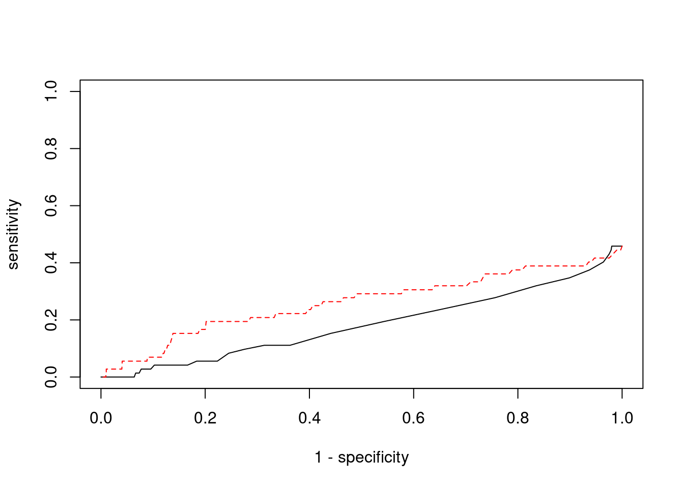

Version	Author	Date
3a7fbc1	wesleycrouse	2021-09-08

Sensitivity, specificity and precision for silver standard genes - bystanders only

This section first uses all silver standard genes to identify bystander genes within 1Mb. The silver standard and bystander gene lists are then subset to only genes with imputed expression in this analysis. Then, the ctwas and TWAS gene lists from this analysis are subset to only genes that are in the (subset) silver standard and bystander genes. These gene lists are then used to compute sensitivity, specificity and precision for ctwas and TWAS.

library(biomaRt)
library(GenomicRanges)

Loading required package: stats4

Loading required package: BiocGenerics

Loading required package: parallel


Attaching package: 'BiocGenerics'

The following objects are masked from 'package:parallel':

    clusterApply, clusterApplyLB, clusterCall, clusterEvalQ,
    clusterExport, clusterMap, parApply, parCapply, parLapply,
    parLapplyLB, parRapply, parSapply, parSapplyLB

The following objects are masked from 'package:stats':

    IQR, mad, sd, var, xtabs

The following objects are masked from 'package:base':

    anyDuplicated, append, as.data.frame, basename, cbind,
    colnames, dirname, do.call, duplicated, eval, evalq, Filter,
    Find, get, grep, grepl, intersect, is.unsorted, lapply, Map,
    mapply, match, mget, order, paste, pmax, pmax.int, pmin,
    pmin.int, Position, rank, rbind, Reduce, rownames, sapply,
    setdiff, sort, table, tapply, union, unique, unsplit, which,
    which.max, which.min

Loading required package: S4Vectors


Attaching package: 'S4Vectors'

The following object is masked from 'package:base':

    expand.grid

Loading required package: IRanges

Loading required package: GenomeInfoDb

ensembl <- useEnsembl(biomart="ENSEMBL_MART_ENSEMBL", dataset="hsapiens_gene_ensembl")
G_list <- getBM(filters= "chromosome_name", attributes= c("hgnc_symbol","chromosome_name","start_position","end_position","gene_biotype"), values=1:22, mart=ensembl)
G_list <- G_list[G_list$hgnc_symbol!="",]
G_list <- G_list[G_list$gene_biotype %in% c("protein_coding","lncRNA"),]
G_list$start <- G_list$start_position
G_list$end <- G_list$end_position
G_list_granges <- makeGRangesFromDataFrame(G_list, keep.extra.columns=T)

known_annotations_positions <- G_list[G_list$hgnc_symbol %in% known_annotations,]
half_window <- 1000000
known_annotations_positions$start <- known_annotations_positions$start_position - half_window
known_annotations_positions$end <- known_annotations_positions$end_position + half_window
known_annotations_positions$start[known_annotations_positions$start<1] <- 1
known_annotations_granges <- makeGRangesFromDataFrame(known_annotations_positions, keep.extra.columns=T)

bystanders <- findOverlaps(known_annotations_granges,G_list_granges)
bystanders <- unique(subjectHits(bystanders))
bystanders <- G_list$hgnc_symbol[bystanders]
bystanders <- bystanders[!(bystanders %in% known_annotations)]
unrelated_genes <- bystanders

#number of genes in known annotations
print(length(known_annotations))

[1] 72

#number of genes in known annotations with imputed expression
print(sum(known_annotations %in% ctwas_gene_res$genename))

[1] 33

#number of bystander genes
print(length(unrelated_genes))

[1] 1837

#number of bystander genes with imputed expression
print(sum(unrelated_genes %in% ctwas_gene_res$genename))

[1] 799

#remove genes without imputed expression from gene lists
known_annotations <- known_annotations[known_annotations %in% ctwas_gene_res$genename]
unrelated_genes <- unrelated_genes[unrelated_genes %in% ctwas_gene_res$genename]

#assign ctwas and TWAS genes
ctwas_genes <- ctwas_gene_res$genename[ctwas_gene_res$susie_pip>0.8]
twas_genes <- ctwas_gene_res$genename[abs(ctwas_gene_res$z)>sig_thresh]

#significance threshold for TWAS
print(sig_thresh)

[1] 4.570782

#number of ctwas genes
length(ctwas_genes)

[1] 2

#number of ctwas genes in known annotations or bystanders
sum(ctwas_genes %in% c(known_annotations, unrelated_genes))

[1] 0

#number of ctwas genes
length(twas_genes)

[1] 32

#number of TWAS genes
sum(twas_genes %in% c(known_annotations, unrelated_genes))

[1] 4

#remove genes not in known or bystander lists from results
ctwas_genes <- ctwas_genes[ctwas_genes %in% c(known_annotations, unrelated_genes)]
twas_genes <- twas_genes[twas_genes %in% c(known_annotations, unrelated_genes)]

#sensitivity / recall
sensitivity <- rep(NA,2)
names(sensitivity) <- c("ctwas", "TWAS")
sensitivity["ctwas"] <- sum(ctwas_genes %in% known_annotations)/length(known_annotations)
sensitivity["TWAS"] <- sum(twas_genes %in% known_annotations)/length(known_annotations)
sensitivity

ctwas  TWAS 
    0     0

#specificity
specificity <- rep(NA,2)
names(specificity) <- c("ctwas", "TWAS")
specificity["ctwas"] <- sum(!(unrelated_genes %in% ctwas_genes))/length(unrelated_genes)
specificity["TWAS"] <- sum(!(unrelated_genes %in% twas_genes))/length(unrelated_genes)
specificity

    ctwas      TWAS 
1.0000000 0.9949937

#precision / PPV
precision <- rep(NA,2)
names(precision) <- c("ctwas", "TWAS")
precision["ctwas"] <- sum(ctwas_genes %in% known_annotations)/length(ctwas_genes)
precision["TWAS"] <- sum(twas_genes %in% known_annotations)/length(twas_genes)
precision

ctwas  TWAS 
  NaN     0

sessionInfo()

R version 3.6.1 (2019-07-05)
Platform: x86_64-pc-linux-gnu (64-bit)
Running under: Scientific Linux 7.4 (Nitrogen)

Matrix products: default
BLAS/LAPACK: /software/openblas-0.2.19-el7-x86_64/lib/libopenblas_haswellp-r0.2.19.so

locale:
 [1] LC_CTYPE=en_US.UTF-8       LC_NUMERIC=C              
 [3] LC_TIME=en_US.UTF-8        LC_COLLATE=en_US.UTF-8    
 [5] LC_MONETARY=en_US.UTF-8    LC_MESSAGES=en_US.UTF-8   
 [7] LC_PAPER=en_US.UTF-8       LC_NAME=C                 
 [9] LC_ADDRESS=C               LC_TELEPHONE=C            
[11] LC_MEASUREMENT=en_US.UTF-8 LC_IDENTIFICATION=C       

attached base packages:
[1] parallel  stats4    stats     graphics  grDevices utils     datasets 
[8] methods   base     

other attached packages:
 [1] GenomicRanges_1.36.0 GenomeInfoDb_1.20.0  IRanges_2.18.1      
 [4] S4Vectors_0.22.1     BiocGenerics_0.30.0  biomaRt_2.40.1      
 [7] readxl_1.3.1         WebGestaltR_0.4.4    disgenet2r_0.99.2   
[10] enrichR_3.0          cowplot_1.0.0        ggplot2_3.3.3       

loaded via a namespace (and not attached):
 [1] bitops_1.0-6           fs_1.3.1               bit64_4.0.5           
 [4] doParallel_1.0.16      progress_1.2.2         httr_1.4.1            
 [7] rprojroot_2.0.2        tools_3.6.1            doRNG_1.8.2           
[10] utf8_1.2.1             R6_2.5.0               DBI_1.1.1             
[13] colorspace_1.4-1       withr_2.4.1            tidyselect_1.1.0      
[16] prettyunits_1.0.2      bit_4.0.4              curl_3.3              
[19] compiler_3.6.1         git2r_0.26.1           Biobase_2.44.0        
[22] labeling_0.3           scales_1.1.0           readr_1.4.0           
[25] stringr_1.4.0          apcluster_1.4.8        digest_0.6.20         
[28] rmarkdown_1.13         svglite_1.2.2          XVector_0.24.0        
[31] pkgconfig_2.0.3        htmltools_0.3.6        fastmap_1.1.0         
[34] rlang_0.4.11           RSQLite_2.2.7          farver_2.1.0          
[37] generics_0.0.2         jsonlite_1.6           dplyr_1.0.7           
[40] RCurl_1.98-1.1         magrittr_2.0.1         GenomeInfoDbData_1.2.1
[43] Matrix_1.2-18          Rcpp_1.0.6             munsell_0.5.0         
[46] fansi_0.5.0            gdtools_0.1.9          lifecycle_1.0.0       
[49] stringi_1.4.3          whisker_0.3-2          yaml_2.2.0            
[52] zlibbioc_1.30.0        plyr_1.8.4             grid_3.6.1            
[55] blob_1.2.1             promises_1.0.1         crayon_1.4.1          
[58] lattice_0.20-38        hms_1.1.0              knitr_1.23            
[61] pillar_1.6.1           igraph_1.2.4.1         rjson_0.2.20          
[64] rngtools_1.5           reshape2_1.4.3         codetools_0.2-16      
[67] XML_3.98-1.20          glue_1.4.2             evaluate_0.14         
[70] data.table_1.14.0      vctrs_0.3.8            httpuv_1.5.1          
[73] foreach_1.5.1          cellranger_1.1.0       gtable_0.3.0          
[76] purrr_0.3.4            assertthat_0.2.1       cachem_1.0.5          
[79] xfun_0.8               later_0.8.0            tibble_3.1.2          
[82] iterators_1.0.13       AnnotationDbi_1.46.0   memoise_2.0.0         
[85] workflowr_1.6.2        ellipsis_0.3.2

Diabetes diagnosed by doctor - Liver

wesleycrouse

2021-09-7