Diabetes diagnosed by doctor - Adipose_Visceral_Omentum
wesleycrouse
2021-09-7
Last updated: 2021-09-13
Checks: 7 0
Knit directory: ctwas_applied/
This reproducible R Markdown analysis was created with workflowr (version 1.6.2). The Checks tab describes the reproducibility checks that were applied when the results were created. The Past versions tab lists the development history.
Great! Since the R Markdown file has been committed to the Git repository, you know the exact version of the code that produced these results.
Great job! The global environment was empty. Objects defined in the global environment can affect the analysis in your R Markdown file in unknown ways. For reproduciblity it’s best to always run the code in an empty environment.
The command set.seed(20210726) was run prior to running the code in the R Markdown file. Setting a seed ensures that any results that rely on randomness, e.g. subsampling or permutations, are reproducible.
Great job! Recording the operating system, R version, and package versions is critical for reproducibility.
Nice! There were no cached chunks for this analysis, so you can be confident that you successfully produced the results during this run.
Great job! Using relative paths to the files within your workflowr project makes it easier to run your code on other machines.
Great! You are using Git for version control. Tracking code development and connecting the code version to the results is critical for reproducibility.
The results in this page were generated with repository version 72c8ef7. See the Past versions tab to see a history of the changes made to the R Markdown and HTML files.
Note that you need to be careful to ensure that all relevant files for the analysis have been committed to Git prior to generating the results (you can use wflow_publish or wflow_git_commit). workflowr only checks the R Markdown file, but you know if there are other scripts or data files that it depends on. Below is the status of the Git repository when the results were generated:
working directory clean
Note that any generated files, e.g. HTML, png, CSS, etc., are not included in this status report because it is ok for generated content to have uncommitted changes.
These are the previous versions of the repository in which changes were made to the R Markdown (analysis/ukb-a-306_Adipose_Visceral_Omentum_known.Rmd) and HTML (docs/ukb-a-306_Adipose_Visceral_Omentum_known.html) files. If you’ve configured a remote Git repository (see ?wflow_git_remote), click on the hyperlinks in the table below to view the files as they were in that past version.
| File | Version | Author | Date | Message |
|---|---|---|---|---|
| Rmd | 72c8ef7 | wesleycrouse | 2021-09-13 | changing mart for biomart |
| Rmd | a49c40e | wesleycrouse | 2021-09-13 | updating with bystander analysis |
| html | 7e22565 | wesleycrouse | 2021-09-13 | updating reports |
| html | 3a7fbc1 | wesleycrouse | 2021-09-08 | generating reports for known annotations |
| Rmd | cbf7408 | wesleycrouse | 2021-09-08 | adding enrichment to reports |
Overview
These are the results of a ctwas analysis of the UK Biobank trait Diabetes diagnosed by doctor using Adipose_Visceral_Omentum gene weights.
The GWAS was conducted by the Neale Lab, and the biomarker traits we analyzed are discussed here. Summary statistics were obtained from IEU OpenGWAS using GWAS ID: ukb-a-306. Results were obtained from from IEU rather than Neale Lab because they are in a standardard format (GWAS VCF). Note that 3 of the 34 biomarker traits were not available from IEU and were excluded from analysis.
The weights are mashr GTEx v8 models on Adipose_Visceral_Omentum eQTL obtained from PredictDB. We performed a full harmonization of the variants, including recovering strand ambiguous variants. This procedure is discussed in a separate document. (TO-DO: add report that describes harmonization)
LD matrices were computed from a 10% subset of Neale lab subjects. Subjects were matched using the plate and well information from genotyping. We included only biallelic variants with MAF>0.01 in the original Neale Lab GWAS. (TO-DO: add more details [number of subjects, variants, etc])
Weight QC
TO-DO: add enhanced QC reporting (total number of weights, why each variant was missing for all genes)
qclist_all <- list()

qc_files <- paste0(results_dir, "/", list.files(results_dir, pattern="exprqc.Rd"))

for (i in 1:length(qc_files)){
  load(qc_files[i])
  chr <- unlist(strsplit(rev(unlist(strsplit(qc_files[i], "_")))[1], "[.]"))[1]
  qclist_all[[chr]] <- cbind(do.call(rbind, lapply(qclist,unlist)), as.numeric(substring(chr,4)))
}

qclist_all <- data.frame(do.call(rbind, qclist_all))
colnames(qclist_all)[ncol(qclist_all)] <- "chr"

rm(qclist, wgtlist, z_gene_chr)

#number of imputed weights
nrow(qclist_all)
[1] 12185#number of imputed weights by chromosome
table(qclist_all$chr)
   1    2    3    4    5    6    7    8    9   10   11   12   13   14   15
1194  835  712  475  563  699  615  440  443  493  756  683  238  409  386
  16   17   18   19   20   21   22
 560  761  189  944  358  140  292
#proportion of imputed weights without missing variants
mean(qclist_all$nmiss==0)[1] 0.7384489Load ctwas results
#load ctwas results
ctwas_res <- data.table::fread(paste0(results_dir, "/", analysis_id, "_ctwas.susieIrss.txt"))

#make unique identifier for regions
ctwas_res$region_tag <- paste(ctwas_res$region_tag1, ctwas_res$region_tag2, sep="_")

#load z scores for SNPs and collect sample size
load(paste0(results_dir, "/", analysis_id, "_expr_z_snp.Rd"))

sample_size <- z_snp$ss
sample_size <- as.numeric(names(which.max(table(sample_size))))

#compute PVE for each gene/SNP
ctwas_res$PVE = ctwas_res$susie_pip*ctwas_res$mu2/sample_size

#separate gene and SNP results
ctwas_gene_res <- ctwas_res[ctwas_res$type == "gene", ]
ctwas_gene_res <- data.frame(ctwas_gene_res)
ctwas_snp_res <- ctwas_res[ctwas_res$type == "SNP", ]
ctwas_snp_res <- data.frame(ctwas_snp_res)

#add gene information to results
sqlite <- RSQLite::dbDriver("SQLite")
db = RSQLite::dbConnect(sqlite, paste0("/project2/compbio/predictdb/mashr_models/mashr_", weight, ".db"))
query <- function(...) RSQLite::dbGetQuery(db, ...)
gene_info <- query("select gene, genename from extra")
gene_info <- query("select gene, genename, gene_type from extra")
RSQLite::dbDisconnect(db)

ctwas_gene_res <- cbind(ctwas_gene_res, gene_info[sapply(ctwas_gene_res$id, match, gene_info$gene), c("genename", "gene_type")])

#add z scores to results
load(paste0(results_dir, "/", analysis_id, "_expr_z_gene.Rd"))
ctwas_gene_res$z <- z_gene[ctwas_gene_res$id,]$z

z_snp <- z_snp[z_snp$id %in% ctwas_snp_res$id,]
ctwas_snp_res$z <- z_snp$z[match(ctwas_snp_res$id, z_snp$id)]

#formatting and rounding for tables
ctwas_gene_res$z <- round(ctwas_gene_res$z,2)
ctwas_snp_res$z <- round(ctwas_snp_res$z,2)
ctwas_gene_res$susie_pip <- round(ctwas_gene_res$susie_pip,3)
ctwas_snp_res$susie_pip <- round(ctwas_snp_res$susie_pip,3)
ctwas_gene_res$mu2 <- round(ctwas_gene_res$mu2,2)
ctwas_snp_res$mu2 <- round(ctwas_snp_res$mu2,2)
ctwas_gene_res$PVE <- signif(ctwas_gene_res$PVE, 2)
ctwas_snp_res$PVE <- signif(ctwas_snp_res$PVE, 2)

#merge gene and snp results with added information
ctwas_snp_res$genename=NA
ctwas_snp_res$gene_type=NA

ctwas_res <- rbind(ctwas_gene_res,
                   ctwas_snp_res[,colnames(ctwas_gene_res)])

#store columns to report
report_cols <- colnames(ctwas_gene_res)[!(colnames(ctwas_gene_res) %in% c("type", "region_tag1", "region_tag2", "cs_index", "gene_type", "z_flag", "id", "chrom", "pos"))]
first_cols <- c("genename", "region_tag")
report_cols <- c(first_cols, report_cols[!(report_cols %in% first_cols)])

report_cols_snps <- c("id", report_cols[-1])

#get number of SNPs from s1 results; adjust for thin
ctwas_res_s1 <- data.table::fread(paste0(results_dir, "/", analysis_id, "_ctwas.s1.susieIrss.txt"))
n_snps <- sum(ctwas_res_s1$type=="SNP")/thin
rm(ctwas_res_s1)
Check convergence of parameters
library(ggplot2)
library(cowplot)
********************************************************Note: As of version 1.0.0, cowplot does not change the default ggplot2 theme anymore. To recover the previous behavior, execute:
theme_set(theme_cowplot())********************************************************load(paste0(results_dir, "/", analysis_id, "_ctwas.s2.susieIrssres.Rd"))
df <- data.frame(niter = rep(1:ncol(group_prior_rec), 2),
value = c(group_prior_rec[1,], group_prior_rec[2,]),
group = rep(c("Gene", "SNP"), each = ncol(group_prior_rec)))
df$group <- as.factor(df$group)
df$value[df$group=="SNP"] <- df$value[df$group=="SNP"]*thin #adjust parameter to account for thin argument
p_pi <- ggplot(df, aes(x=niter, y=value, group=group)) +
geom_line(aes(color=group)) +
geom_point(aes(color=group)) +
xlab("Iteration") + ylab(bquote(pi)) +
ggtitle("Prior mean") +
theme_cowplot()
df <- data.frame(niter = rep(1:ncol(group_prior_var_rec), 2),
value = c(group_prior_var_rec[1,], group_prior_var_rec[2,]),
group = rep(c("Gene", "SNP"), each = ncol(group_prior_var_rec)))
df$group <- as.factor(df$group)
p_sigma2 <- ggplot(df, aes(x=niter, y=value, group=group)) +
geom_line(aes(color=group)) +
geom_point(aes(color=group)) +
xlab("Iteration") + ylab(bquote(sigma^2)) +
ggtitle("Prior variance") +
theme_cowplot()
plot_grid(p_pi, p_sigma2)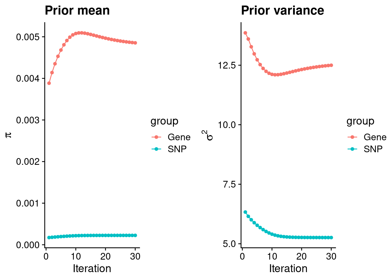
| Version | Author | Date |
|---|---|---|
| 3a7fbc1 | wesleycrouse | 2021-09-08 |
#estimated group prior
estimated_group_prior <- group_prior_rec[,ncol(group_prior_rec)]
names(estimated_group_prior) <- c("gene", "snp")
estimated_group_prior["snp"] <- estimated_group_prior["snp"]*thin #adjust parameter to account for thin argument
print(estimated_group_prior)
gene snp
0.0048541631 0.0002254267 #estimated group prior variance
estimated_group_prior_var <- group_prior_var_rec[,ncol(group_prior_var_rec)]
names(estimated_group_prior_var) <- c("gene", "snp")
print(estimated_group_prior_var) gene snp
12.49871 5.26040 #report sample size
print(sample_size)[1] 336473#report group size
group_size <- c(nrow(ctwas_gene_res), n_snps)
print(group_size)[1] 12185 7535010#estimated group PVE
estimated_group_pve <- estimated_group_prior_var*estimated_group_prior*group_size/sample_size #check PVE calculation
names(estimated_group_pve) <- c("gene", "snp")
print(estimated_group_pve) gene snp
0.002197125 0.026555703 #compare sum(PIP*mu2/sample_size) with above PVE calculation
c(sum(ctwas_gene_res$PVE),sum(ctwas_snp_res$PVE))[1] 0.01047966 0.40446400Genes with highest PIPs
#distribution of PIPs
hist(ctwas_gene_res$susie_pip, xlim=c(0,1), main="Distribution of Gene PIPs")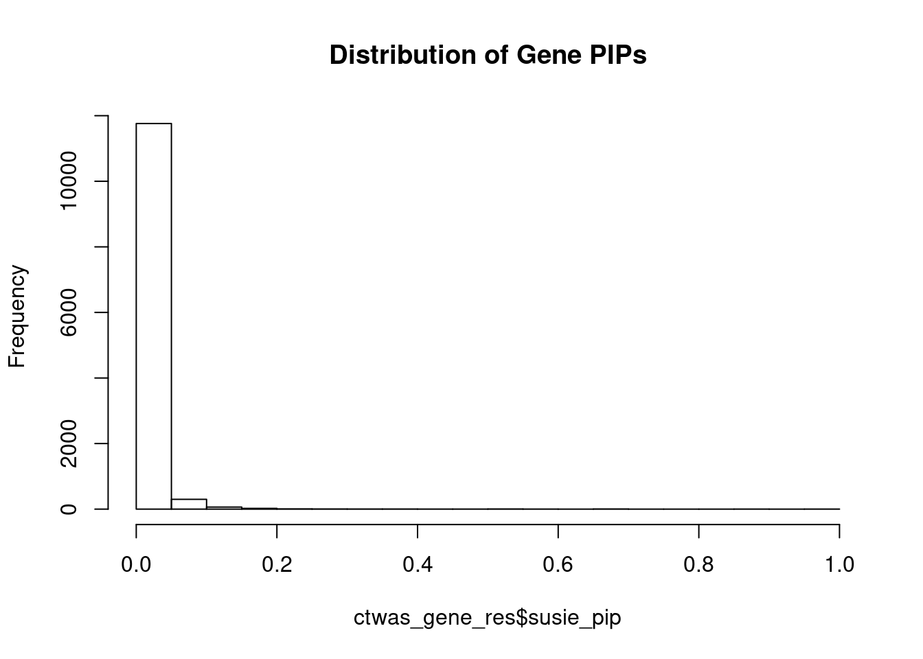
| Version | Author | Date |
|---|---|---|
| 3a7fbc1 | wesleycrouse | 2021-09-08 |
#genes with PIP>0.8 or 20 highest PIPs
head(ctwas_gene_res[order(-ctwas_gene_res$susie_pip),report_cols], max(sum(ctwas_gene_res$susie_pip>0.8), 20))
genename region_tag susie_pip mu2 PVE z
3645 CCND2 12_4 0.999 95.50 2.8e-04 9.93
7057 JAZF1 7_23 0.956 57.24 1.6e-04 7.84
13794 GTF2I 7_48 0.897 27.52 7.3e-05 -5.05
12711 XXbac-BPG13B8.10 6_23 0.851 30.70 7.8e-05 -5.44
7924 INHBB 2_70 0.767 26.01 5.9e-05 -4.47
2722 WFS1 4_7 0.685 65.10 1.3e-04 -8.31
11442 ZNF34 8_94 0.677 26.06 5.2e-05 -4.72
9611 PEAK1 15_36 0.674 32.80 6.6e-05 5.41
7075 NUS1 6_78 0.661 23.52 4.6e-05 4.44
7757 C16orf59 16_2 0.619 26.95 5.0e-05 -3.88
12763 HLA-DPA1 6_27 0.566 25.85 4.3e-05 -4.09
10525 UBE2E2 3_17 0.560 28.10 4.7e-05 -5.07
1401 PABPC4 1_24 0.543 28.48 4.6e-05 4.88
13192 LINC01184 5_78 0.543 23.10 3.7e-05 -4.05
3656 CCDC92 12_75 0.542 28.36 4.6e-05 4.36
4453 LRRC17 7_63 0.506 29.41 4.4e-05 5.00
7159 RAB6B 3_83 0.504 28.45 4.3e-05 3.94
5451 FLOT1 6_24 0.494 773.81 1.1e-03 -5.84
3941 ZMIZ2 7_33 0.485 23.24 3.4e-05 -4.09
5583 TACC2 10_76 0.411 29.32 3.6e-05 3.93Genes with largest effect sizes
#plot PIP vs effect size
plot(ctwas_gene_res$susie_pip, ctwas_gene_res$mu2, xlab="PIP", ylab="mu^2", main="Gene PIPs vs Effect Size")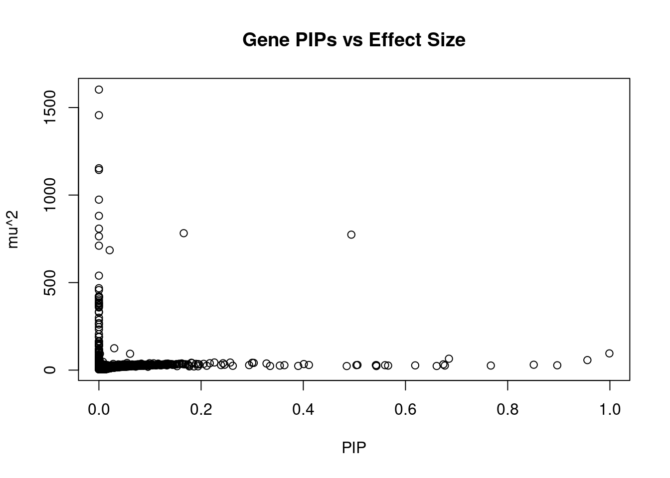
| Version | Author | Date |
|---|---|---|
| 3a7fbc1 | wesleycrouse | 2021-09-08 |
#genes with 20 largest effect sizes
head(ctwas_gene_res[order(-ctwas_gene_res$mu2),report_cols],20)
genename region_tag susie_pip mu2 PVE z
14144 XXbac-BPG181B23.7 6_25 0.000 1602.60 0.0e+00 7.46
12971 HLA-DQA2 6_26 0.000 1456.34 0.0e+00 -11.46
12069 PSORS1C2 6_25 0.000 1153.09 0.0e+00 -4.27
12223 HCG27 6_25 0.000 1143.56 0.0e+00 -5.72
10255 HLA-DQB1 6_26 0.000 973.83 0.0e+00 4.57
11153 ZKSCAN4 6_22 0.000 881.27 0.0e+00 -3.56
13767 RP1-265C24.8 6_22 0.000 808.22 0.0e+00 -2.61
6481 PPP1R18 6_24 0.166 782.18 3.9e-04 5.70
5451 FLOT1 6_24 0.494 773.81 1.1e-03 -5.84
12698 HCG22 6_25 0.000 764.37 0.0e+00 4.48
11557 ZSCAN26 6_22 0.000 710.76 0.0e+00 3.80
12407 LINC00243 6_24 0.021 684.94 4.3e-05 -5.79
12780 CYP21A2 6_26 0.000 539.54 0.0e+00 -5.80
12068 CCHCR1 6_25 0.000 467.98 0.0e+00 -6.10
12024 RNF5 6_26 0.000 457.12 0.0e+00 6.17
12061 NFKBIL1 6_25 0.000 422.02 0.0e+00 -0.82
12629 LTA 6_25 0.000 420.97 0.0e+00 4.47
12085 TRIM31 6_24 0.000 420.73 2.8e-16 3.23
5450 TCF19 6_25 0.000 418.64 0.0e+00 -4.36
11593 ZNF165 6_22 0.000 417.66 0.0e+00 2.64Genes with highest PVE
#genes with 20 highest pve
head(ctwas_gene_res[order(-ctwas_gene_res$PVE),report_cols],20)
genename region_tag susie_pip mu2 PVE z
5451 FLOT1 6_24 0.494 773.81 1.1e-03 -5.84
6481 PPP1R18 6_24 0.166 782.18 3.9e-04 5.70
3645 CCND2 12_4 0.999 95.50 2.8e-04 9.93
7057 JAZF1 7_23 0.956 57.24 1.6e-04 7.84
2722 WFS1 4_7 0.685 65.10 1.3e-04 -8.31
12711 XXbac-BPG13B8.10 6_23 0.851 30.70 7.8e-05 -5.44
13794 GTF2I 7_48 0.897 27.52 7.3e-05 -5.05
9611 PEAK1 15_36 0.674 32.80 6.6e-05 5.41
7924 INHBB 2_70 0.767 26.01 5.9e-05 -4.47
11442 ZNF34 8_94 0.677 26.06 5.2e-05 -4.72
7757 C16orf59 16_2 0.619 26.95 5.0e-05 -3.88
10525 UBE2E2 3_17 0.560 28.10 4.7e-05 -5.07
1401 PABPC4 1_24 0.543 28.48 4.6e-05 4.88
7075 NUS1 6_78 0.661 23.52 4.6e-05 4.44
3656 CCDC92 12_75 0.542 28.36 4.6e-05 4.36
4453 LRRC17 7_63 0.506 29.41 4.4e-05 5.00
7159 RAB6B 3_83 0.504 28.45 4.3e-05 3.94
12763 HLA-DPA1 6_27 0.566 25.85 4.3e-05 -4.09
12407 LINC00243 6_24 0.021 684.94 4.3e-05 -5.79
2319 CRTC1 19_15 0.401 34.53 4.1e-05 -3.95Genes with largest z scores
#genes with 20 largest z scores
head(ctwas_gene_res[order(-abs(ctwas_gene_res$z)),report_cols],20)
genename region_tag susie_pip mu2 PVE z
12971 HLA-DQA2 6_26 0.000 1456.34 0.0e+00 -11.46
3645 CCND2 12_4 0.999 95.50 2.8e-04 9.93
12038 EHMT2 6_26 0.000 191.48 0.0e+00 -8.33
2722 WFS1 4_7 0.685 65.10 1.3e-04 -8.31
7057 JAZF1 7_23 0.956 57.24 1.6e-04 7.84
14144 XXbac-BPG181B23.7 6_25 0.000 1602.60 0.0e+00 7.46
12315 DDAH2 6_26 0.000 332.93 0.0e+00 7.21
12017 PSMB8 6_27 0.008 47.06 1.1e-06 -7.14
12058 AIF1 6_26 0.000 378.59 0.0e+00 -6.65
12046 MSH5 6_26 0.000 369.97 0.0e+00 6.63
12314 CLIC1 6_26 0.000 369.97 0.0e+00 6.63
12054 APOM 6_26 0.000 362.46 0.0e+00 6.52
14565 LINC01126 2_27 0.055 40.71 6.7e-06 6.23
12021 NOTCH4 6_26 0.000 386.39 0.0e+00 6.17
12024 RNF5 6_26 0.000 457.12 0.0e+00 6.17
13169 C4A 6_26 0.000 394.53 0.0e+00 6.15
12068 CCHCR1 6_25 0.000 467.98 0.0e+00 -6.10
11136 KCNJ11 11_12 0.328 37.80 3.7e-05 -5.91
5451 FLOT1 6_24 0.494 773.81 1.1e-03 -5.84
12780 CYP21A2 6_26 0.000 539.54 0.0e+00 -5.80Comparing z scores and PIPs
#set nominal signifiance threshold for z scores
alpha <- 0.05

#bonferroni adjusted threshold for z scores
sig_thresh <- qnorm(1-(alpha/nrow(ctwas_gene_res)/2), lower=T)

#Q-Q plot for z scores
obs_z <- ctwas_gene_res$z[order(ctwas_gene_res$z)]
exp_z <- qnorm((1:nrow(ctwas_gene_res))/nrow(ctwas_gene_res))

plot(exp_z, obs_z, xlab="Expected z", ylab="Observed z", main="Gene z score Q-Q plot")
abline(a=0,b=1)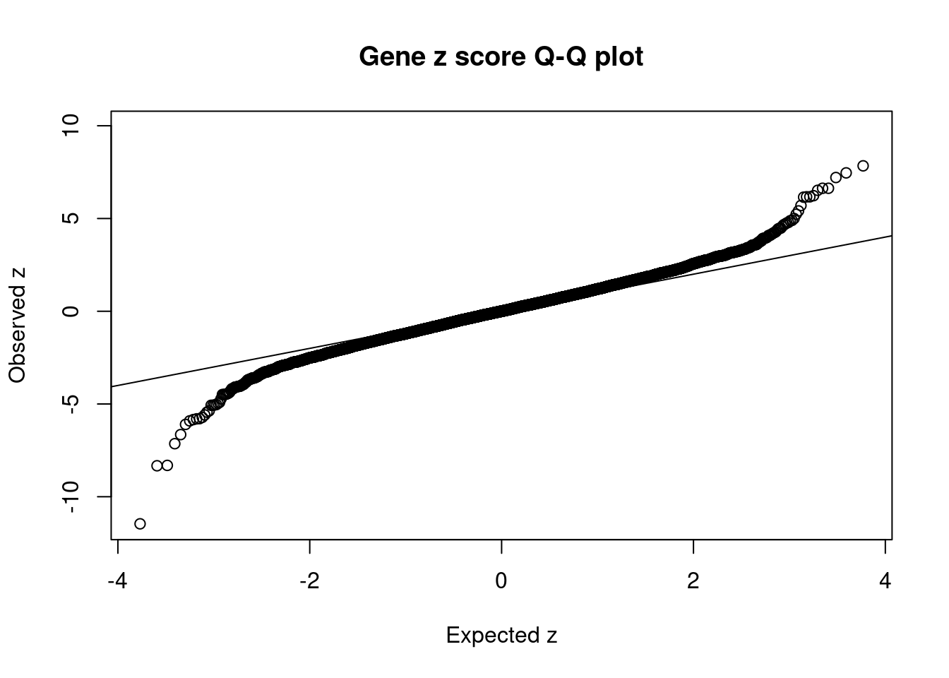
| Version | Author | Date |
|---|---|---|
| 3a7fbc1 | wesleycrouse | 2021-09-08 |
#plot z score vs PIP
plot(abs(ctwas_gene_res$z), ctwas_gene_res$susie_pip, xlab="abs(z)", ylab="PIP")
abline(v=sig_thresh, col="red", lty=2)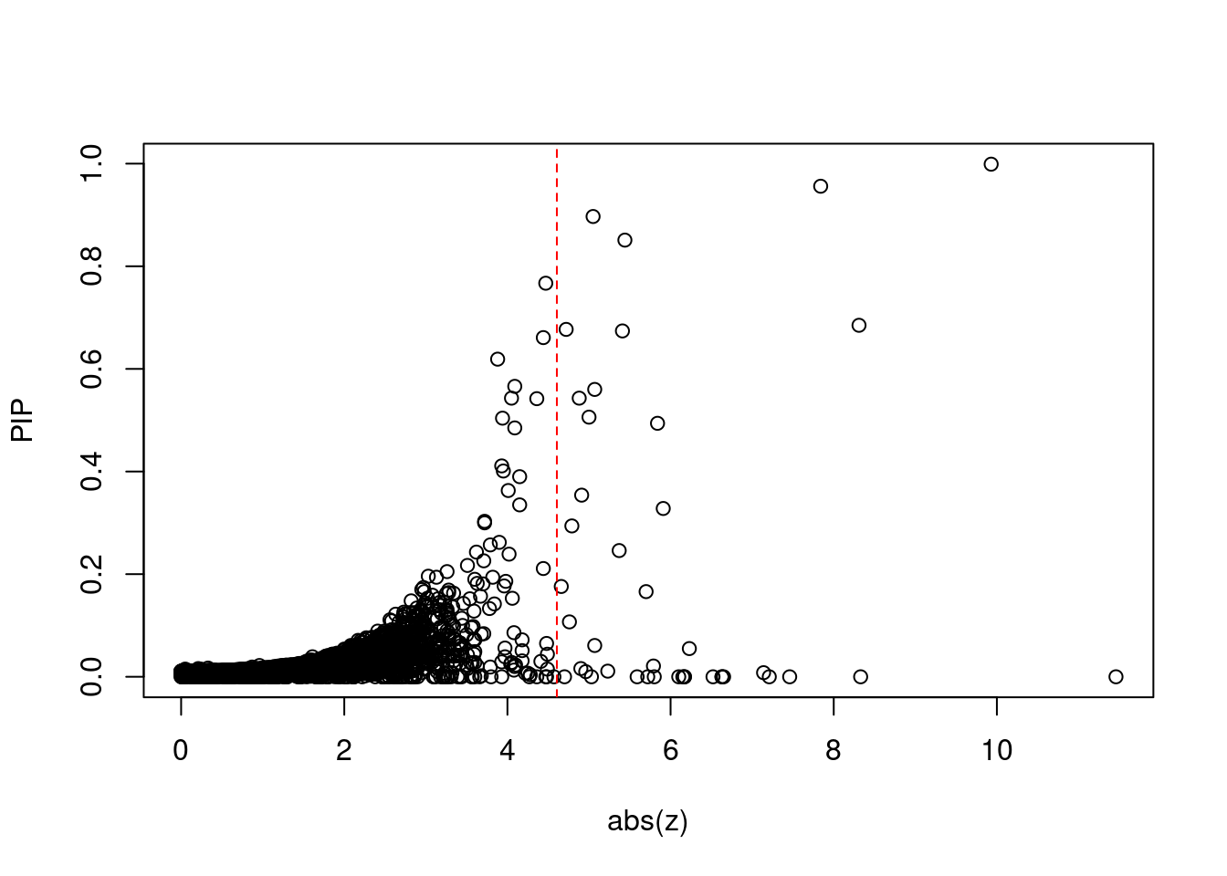
| Version | Author | Date |
|---|---|---|
| 3a7fbc1 | wesleycrouse | 2021-09-08 |
#proportion of significant z scores
mean(abs(ctwas_gene_res$z) > sig_thresh)
[1] 0.003446861#genes with most significant z scores
head(ctwas_gene_res[order(-abs(ctwas_gene_res$z)),report_cols],20) genename region_tag susie_pip mu2 PVE z
12971 HLA-DQA2 6_26 0.000 1456.34 0.0e+00 -11.46
3645 CCND2 12_4 0.999 95.50 2.8e-04 9.93
12038 EHMT2 6_26 0.000 191.48 0.0e+00 -8.33
2722 WFS1 4_7 0.685 65.10 1.3e-04 -8.31
7057 JAZF1 7_23 0.956 57.24 1.6e-04 7.84
14144 XXbac-BPG181B23.7 6_25 0.000 1602.60 0.0e+00 7.46
12315 DDAH2 6_26 0.000 332.93 0.0e+00 7.21
12017 PSMB8 6_27 0.008 47.06 1.1e-06 -7.14
12058 AIF1 6_26 0.000 378.59 0.0e+00 -6.65
12046 MSH5 6_26 0.000 369.97 0.0e+00 6.63
12314 CLIC1 6_26 0.000 369.97 0.0e+00 6.63
12054 APOM 6_26 0.000 362.46 0.0e+00 6.52
14565 LINC01126 2_27 0.055 40.71 6.7e-06 6.23
12021 NOTCH4 6_26 0.000 386.39 0.0e+00 6.17
12024 RNF5 6_26 0.000 457.12 0.0e+00 6.17
13169 C4A 6_26 0.000 394.53 0.0e+00 6.15
12068 CCHCR1 6_25 0.000 467.98 0.0e+00 -6.10
11136 KCNJ11 11_12 0.328 37.80 3.7e-05 -5.91
5451 FLOT1 6_24 0.494 773.81 1.1e-03 -5.84
12780 CYP21A2 6_26 0.000 539.54 0.0e+00 -5.80Locus plots for genes and SNPs
ctwas_gene_res_sortz <- ctwas_gene_res[order(-abs(ctwas_gene_res$z)),]

n_plots <- 5
for (region_tag_plot in head(unique(ctwas_gene_res_sortz$region_tag), n_plots)){
  ctwas_res_region <-  ctwas_res[ctwas_res$region_tag==region_tag_plot,]
  start <- min(ctwas_res_region$pos)
  end <- max(ctwas_res_region$pos)

  ctwas_res_region <- ctwas_res_region[order(ctwas_res_region$pos),]
  ctwas_res_region_gene <- ctwas_res_region[ctwas_res_region$type=="gene",]
  ctwas_res_region_snp <- ctwas_res_region[ctwas_res_region$type=="SNP",]

  #region name
  print(paste0("Region: ", region_tag_plot))

  #table of genes in region
  print(ctwas_res_region_gene[,report_cols])

  par(mfrow=c(4,1))

  #gene z scores
  plot(ctwas_res_region_gene$pos, abs(ctwas_res_region_gene$z), xlab="Position", ylab="abs(gene_z)", xlim=c(start,end),
   ylim=c(0,max(sig_thresh, abs(ctwas_res_region_gene$z))),
   main=paste0("Region: ", region_tag_plot))
  abline(h=sig_thresh,col="red",lty=2)

  #significance threshold for SNPs
  alpha_snp <- 5*10^(-8)
  sig_thresh_snp <- qnorm(1-alpha_snp/2, lower=T)

  #snp z scores
  plot(ctwas_res_region_snp$pos, abs(ctwas_res_region_snp$z), xlab="Position", ylab="abs(snp_z)",xlim=c(start,end),
   ylim=c(0,max(sig_thresh_snp, max(abs(ctwas_res_region_snp$z)))))
  abline(h=sig_thresh_snp,col="purple",lty=2)

  #gene pips
  plot(ctwas_res_region_gene$pos, ctwas_res_region_gene$susie_pip, xlab="Position", ylab="Gene PIP", xlim=c(start,end), ylim=c(0,1))
  abline(h=0.8,col="blue",lty=2)

  #snp pips
  plot(ctwas_res_region_snp$pos, ctwas_res_region_snp$susie_pip, xlab="Position", ylab="SNP PIP", xlim=c(start,end), ylim=c(0,1))
  abline(h=0.8,col="blue",lty=2)
}
[1] "Region: 6_26"
genename region_tag susie_pip mu2 PVE z
12056 BAG6 6_26 0 8.95 0 0.46
12058 AIF1 6_26 0 378.59 0 -6.65
12054 APOM 6_26 0 362.46 0 6.52
12053 C6orf47 6_26 0 34.63 0 -2.10
12052 GPANK1 6_26 0 65.73 0 2.01
12051 CSNK2B 6_26 0 27.95 0 3.21
13028 LY6G5B 6_26 0 30.71 0 0.13
12049 ABHD16A 6_26 0 8.57 0 1.70
12048 LY6G6C 6_26 0 51.60 0 -1.18
12315 DDAH2 6_26 0 332.93 0 7.21
12046 MSH5 6_26 0 369.97 0 6.63
12314 CLIC1 6_26 0 369.97 0 6.63
12695 SAPCD1 6_26 0 36.43 0 1.73
12041 C6orf48 6_26 0 36.07 0 -0.23
12044 VWA7 6_26 0 6.44 0 -0.05
12034 SKIV2L 6_26 0 30.18 0 2.82
12043 VARS 6_26 0 77.96 0 -3.39
12042 LSM2 6_26 0 24.66 0 -0.53
12040 NEU1 6_26 0 8.03 0 -0.93
12038 EHMT2 6_26 0 191.48 0 -8.33
12036 ZBTB12 6_26 0 53.93 0 1.65
13127 CFB 6_26 0 63.45 0 2.81
12032 STK19 6_26 0 44.53 0 1.65
12033 DXO 6_26 0 25.22 0 3.09
13169 C4A 6_26 0 394.53 0 6.15
12780 CYP21A2 6_26 0 539.54 0 -5.80
12309 ATF6B 6_26 0 109.99 0 -5.59
12028 FKBPL 6_26 0 23.45 0 -3.60
12027 PRRT1 6_26 0 106.64 0 -3.12
12492 PPT2 6_26 0 25.68 0 -0.14
12534 C4B 6_26 0 20.05 0 -1.08
13061 EGFL8 6_26 0 25.65 0 -0.17
12024 RNF5 6_26 0 457.12 0 6.17
12023 AGER 6_26 0 403.50 0 -5.03
12021 NOTCH4 6_26 0 386.39 0 6.17
12971 HLA-DQA2 6_26 0 1456.34 0 -11.46
11509 HLA-DQA1 6_26 0 144.50 0 0.28
10255 HLA-DQB1 6_26 0 973.83 0 4.57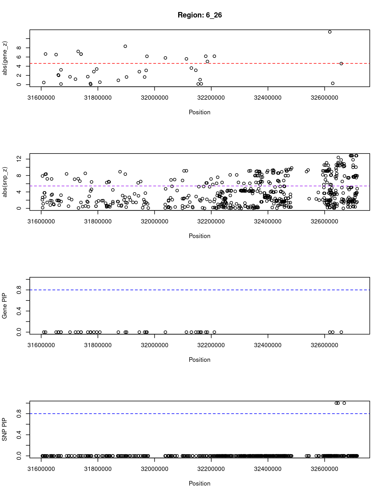
| Version | Author | Date |
|---|---|---|
| 3a7fbc1 | wesleycrouse | 2021-09-08 |
[1] "Region: 12_4"
     genename region_tag susie_pip   mu2     PVE     z
4564  CRACR2A       12_4     0.020 19.92 1.2e-06  1.86
2869   PARP11       12_4     0.019 20.28 1.1e-06 -2.08
3645    CCND2       12_4     0.999 95.50 2.8e-04  9.93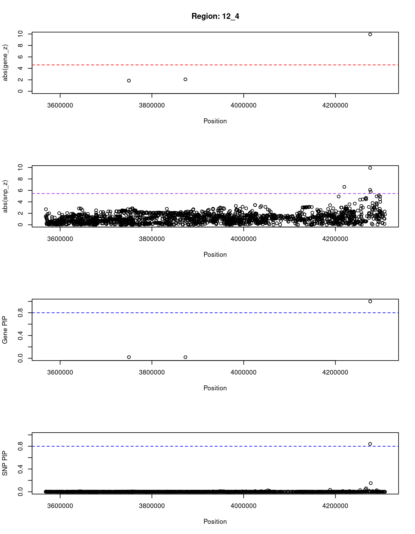
| Version | Author | Date |
|---|---|---|
| 3a7fbc1 | wesleycrouse | 2021-09-08 |
[1] "Region: 4_7"
           genename region_tag susie_pip   mu2     PVE     z
9552           EVC2        4_7     0.020 15.26 9.3e-07 -1.81
898           CRMP1        4_7     0.006  4.65 8.8e-08 -0.11
6999        JAKMIP1        4_7     0.006  4.68 8.9e-08 -0.16
2722           WFS1        4_7     0.685 65.10 1.3e-04 -8.31
930         PPP2R2C        4_7     0.006  4.63 8.7e-08 -0.02
239          MAN2B2        4_7     0.011  9.18 2.9e-07 -0.97
10215        MRFAP1        4_7     0.012 10.63 3.8e-07 -1.24
9249     AC093323.3        4_7     0.006  4.63 8.7e-08  0.06
13343 RP11-539L10.3        4_7     0.007  5.00 9.8e-08 -0.27
13203 RP11-539L10.2        4_7     0.007  5.33 1.1e-07  0.46
8118          S100P        4_7     0.007  4.95 9.6e-08  0.27
10212      MRFAP1L1        4_7     0.085 28.97 7.3e-06  2.61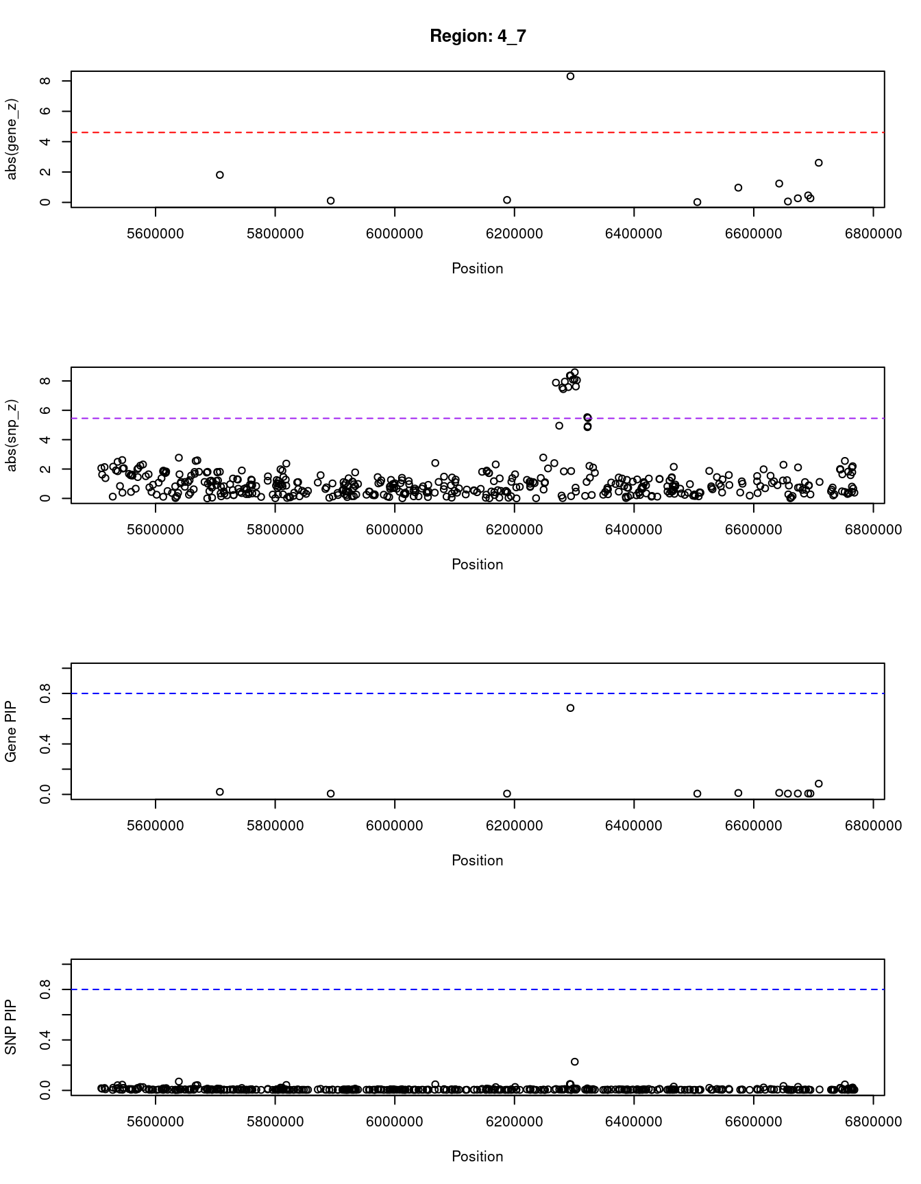
| Version | Author | Date |
|---|---|---|
| 3a7fbc1 | wesleycrouse | 2021-09-08 |
[1] "Region: 7_23"
           genename region_tag susie_pip   mu2     PVE     z
14043 CTD-2227E11.1       7_23     0.005  6.36 9.1e-08 -0.57
500          NFE2L3       7_23     0.004  5.37 6.8e-08  0.43
3947           CBX3       7_23     0.004  4.91 5.9e-08 -0.38
1254          SNX10       7_23     0.043 26.52 3.4e-06  2.50
12405    AC004540.5       7_23     0.040 25.89 3.1e-06  2.38
12842    AC004947.2       7_23     0.006  9.16 1.7e-07  1.21
12494       C7orf71       7_23     0.004  5.53 7.2e-08 -0.37
55            SKAP2       7_23     0.004  4.64 5.5e-08  0.25
2380          HOXA1       7_23     0.005  6.69 9.6e-08  0.78
11641         HOXA4       7_23     0.004  4.75 5.7e-08  0.15
2383          HOXA5       7_23     0.004  4.67 5.5e-08  0.18
2384          HOXA6       7_23     0.004  4.97 6.1e-08 -0.12
3951          HOXA7       7_23     0.004  5.09 6.4e-08 -0.16
1058          HOXA9       7_23     0.005  6.75 1.0e-07  0.65
2390         HIBADH       7_23     0.004  4.65 5.5e-08 -0.30
2391        TAX1BP1       7_23     0.004  4.86 5.8e-08  0.61
7057          JAZF1       7_23     0.956 57.24 1.6e-04  7.84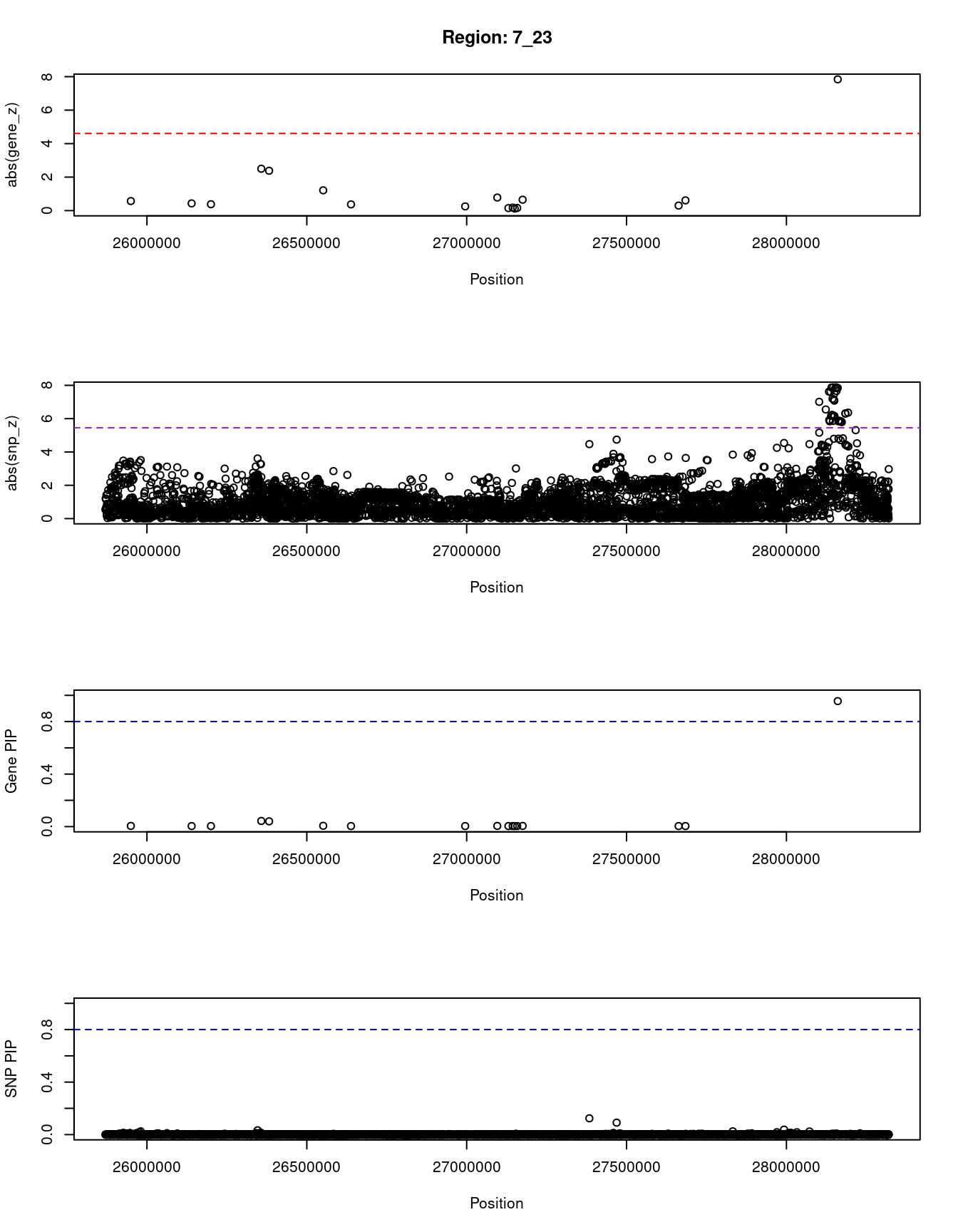
| Version | Author | Date |
|---|---|---|
| 3a7fbc1 | wesleycrouse | 2021-09-08 |
[1] "Region: 6_25"
               genename region_tag susie_pip     mu2 PVE     z
12077              DDR1       6_25         0   64.47   0  3.31
12318            GTF2H4       6_25         0   10.22   0  1.13
5461              VARS2       6_25         0   15.97   0  0.76
11412             SFTA2       6_25         0   17.03   0 -1.28
12698             HCG22       6_25         0  764.37   0  4.48
12070          PSORS1C1       6_25         0  163.78   0 -0.12
12069          PSORS1C2       6_25         0 1153.09   0 -4.27
5450              TCF19       6_25         0  418.64   0 -4.36
12068            CCHCR1       6_25         0  467.98   0 -6.10
12067            POU5F1       6_25         0  116.87   0 -3.42
12223             HCG27       6_25         0 1143.56   0 -5.72
12066             HLA-C       6_25         0  121.31   0 -3.66
12878             HLA-B       6_25         0  141.33   0 -3.26
14144 XXbac-BPG181B23.7       6_25         0 1602.60   0  7.46
12064              MICA       6_25         0  118.76   0 -3.10
12062              MICB       6_25         0  285.71   0 -3.93
12316          ATP6V1G2       6_25         0  357.94   0  0.15
12061           NFKBIL1       6_25         0  422.02   0 -0.82
12629               LTA       6_25         0  420.97   0  4.47
12812               TNF       6_25         0   45.26   0  2.12
12060              LST1       6_25         0  299.44   0 -0.78
12059              NCR3       6_25         0   46.86   0  0.23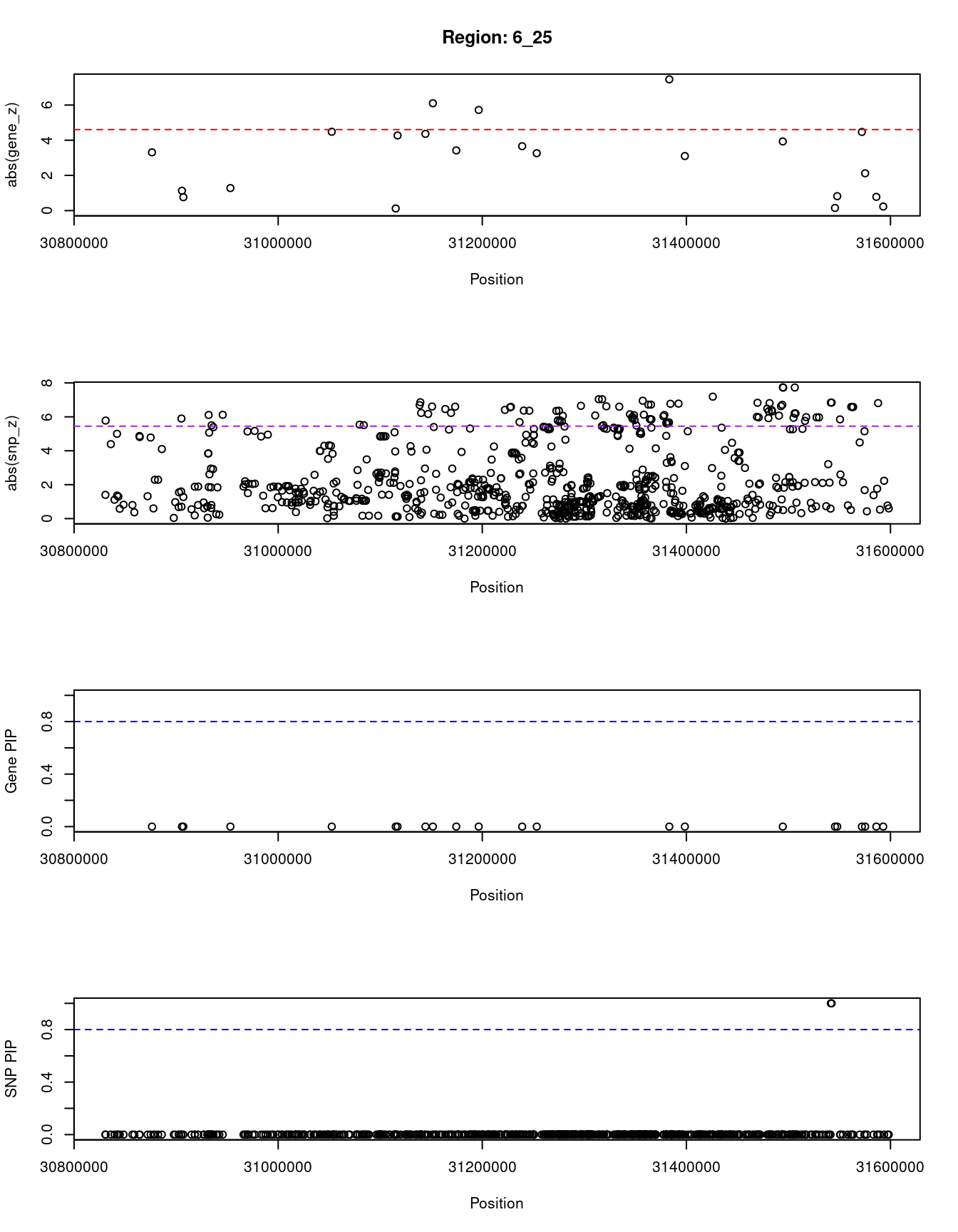
| Version | Author | Date |
|---|---|---|
| 3a7fbc1 | wesleycrouse | 2021-09-08 |
SNPs with highest PIPs
#snps with PIP>0.8 or 20 highest PIPs
head(ctwas_snp_res[order(-ctwas_snp_res$susie_pip),report_cols_snps],
max(sum(ctwas_snp_res$susie_pip>0.8), 20))
id region_tag susie_pip mu2 PVE z
5205 rs56219074 1_13 1.000 62.07 1.8e-04 2.18
37018 rs75222047 1_85 1.000 755.36 2.2e-03 2.91
42580 rs2776714 1_97 1.000 745.72 2.2e-03 -2.78
82161 rs12471681 2_53 1.000 873.56 2.6e-03 -3.05
139434 rs13062973 3_45 1.000 584.80 1.7e-03 -3.60
167435 rs1388475 3_107 1.000 485.85 1.4e-03 2.87
167436 rs13071192 3_107 1.000 463.91 1.4e-03 -3.12
169901 rs28661518 3_112 1.000 915.31 2.7e-03 -3.09
209719 rs2125449 4_79 1.000 954.96 2.8e-03 -3.33
252840 rs3910018 5_51 1.000 778.84 2.3e-03 -2.86
284239 rs2206734 6_15 1.000 83.50 2.5e-04 10.34
286537 rs34662244 6_22 1.000 1627.88 4.8e-03 4.07
286555 rs67297533 6_22 1.000 1591.93 4.7e-03 -4.09
287582 rs2523507 6_25 1.000 4590.62 1.4e-02 6.84
287583 rs2239528 6_25 1.000 4488.64 1.3e-02 -6.84
288108 rs9272679 6_26 1.000 1692.31 5.0e-03 -9.31
288117 rs17612548 6_26 1.000 1768.33 5.3e-03 11.17
288138 rs3134996 6_26 1.000 1743.80 5.2e-03 10.37
288222 rs3916765 6_27 1.000 97.35 2.9e-04 10.72
378881 rs1495743 8_21 1.000 401.73 1.2e-03 3.21
406861 rs16902104 8_83 1.000 1196.48 3.6e-03 3.51
435734 rs7025746 9_53 1.000 369.30 1.1e-03 -3.04
435738 rs2900388 9_53 1.000 362.42 1.1e-03 3.51
471145 rs2019640 10_59 1.000 963.44 2.9e-03 -3.47
471147 rs913647 10_59 1.000 965.88 2.9e-03 3.45
476500 rs12244851 10_70 1.000 255.37 7.6e-04 22.39
484038 rs234856 11_3 1.000 36.93 1.1e-04 -4.94
486071 rs11041828 11_6 1.000 833.29 2.5e-03 2.96
486072 rs4237770 11_6 1.000 851.82 2.5e-03 -2.93
498011 rs113527193 11_30 1.000 437.47 1.3e-03 3.29
498342 rs11603701 11_30 1.000 455.08 1.4e-03 -3.24
612527 rs12912777 15_13 1.000 33.12 9.8e-05 5.53
649018 rs12443634 16_45 1.000 187.57 5.6e-04 -3.47
649025 rs2966092 16_45 1.000 190.07 5.6e-04 3.38
654546 rs4790233 17_5 1.000 197.47 5.9e-04 -3.70
654551 rs8072531 17_5 1.000 198.21 5.9e-04 -3.98
700203 rs73537429 19_15 1.000 265.11 7.9e-04 -2.52
719599 rs2747568 20_20 1.000 1249.50 3.7e-03 3.79
719600 rs2064505 20_20 1.000 1281.35 3.8e-03 -3.92
790569 rs2939608 12_56 1.000 859.88 2.6e-03 -2.96
65949 rs780093 2_16 0.999 41.67 1.2e-04 6.98
429052 rs9410573 9_40 0.999 46.83 1.4e-04 -7.44
661436 rs9906451 17_22 0.999 30.42 9.0e-05 -5.87
573096 rs1327315 13_40 0.994 32.57 9.6e-05 -7.40
378884 rs34537991 8_21 0.993 347.66 1.0e-03 3.06
420340 rs10965243 9_16 0.991 26.37 7.8e-05 -5.41
700205 rs67238925 19_15 0.984 256.19 7.5e-04 2.39
769930 rs3129696 6_24 0.983 1297.54 3.8e-03 -3.92
435737 rs7868850 9_53 0.982 69.98 2.0e-04 0.83
316378 rs138764591 6_89 0.980 23.96 7.0e-05 2.59
288323 rs2857161 6_27 0.976 85.61 2.5e-04 6.21
47621 rs79687284 1_108 0.975 25.29 7.3e-05 5.66
167438 rs13081434 3_107 0.971 444.68 1.3e-03 -2.47
435735 rs4742930 9_53 0.969 286.30 8.2e-04 3.25
537309 rs189339 12_40 0.941 33.16 9.3e-05 -6.27
406860 rs16902103 8_83 0.938 1170.16 3.3e-03 -3.50
484037 rs234852 11_3 0.938 25.87 7.2e-05 3.12
700232 rs2285626 19_15 0.937 115.21 3.2e-04 5.36
153741 rs72964564 3_76 0.931 33.08 9.2e-05 -6.10
471225 rs1977833 10_59 0.927 98.21 2.7e-04 -8.47
29222 rs6679677 1_70 0.920 26.90 7.4e-05 5.33
169902 rs73190822 3_112 0.917 894.42 2.4e-03 3.11
256035 rs10479168 5_59 0.914 26.01 7.1e-05 5.36
573108 rs502027 13_40 0.908 31.56 8.5e-05 7.22
170786 rs6444187 3_114 0.904 25.59 6.9e-05 5.17
204272 rs35518360 4_67 0.875 24.26 6.3e-05 4.70
646261 rs72802395 16_40 0.874 35.53 9.2e-05 -6.35
534358 rs2682323 12_33 0.871 23.95 6.2e-05 4.74
47625 rs340835 1_108 0.853 25.64 6.5e-05 5.52
785884 rs3217792 12_4 0.842 37.00 9.3e-05 -6.10
138700 rs3774723 3_43 0.832 24.62 6.1e-05 -4.84
37037 rs2179109 1_85 0.827 739.23 1.8e-03 -3.03
607429 rs117618513 14_54 0.827 25.11 6.2e-05 -4.96
139422 rs34695932 3_45 0.821 611.97 1.5e-03 4.13
169900 rs62287225 3_112 0.821 894.19 2.2e-03 3.08
654542 rs79425343 17_5 0.821 24.32 5.9e-05 1.15
662491 rs665268 17_25 0.819 26.21 6.4e-05 5.36
159281 rs73148854 3_89 0.816 23.06 5.6e-05 -4.35
604998 rs11160254 14_49 0.806 24.18 5.8e-05 4.55
707260 rs12609461 19_33 0.805 28.90 6.9e-05 5.53SNPs with largest effect sizes
#plot PIP vs effect size
plot(ctwas_snp_res$susie_pip, ctwas_snp_res$mu2, xlab="PIP", ylab="mu^2", main="SNP PIPs vs Effect Size")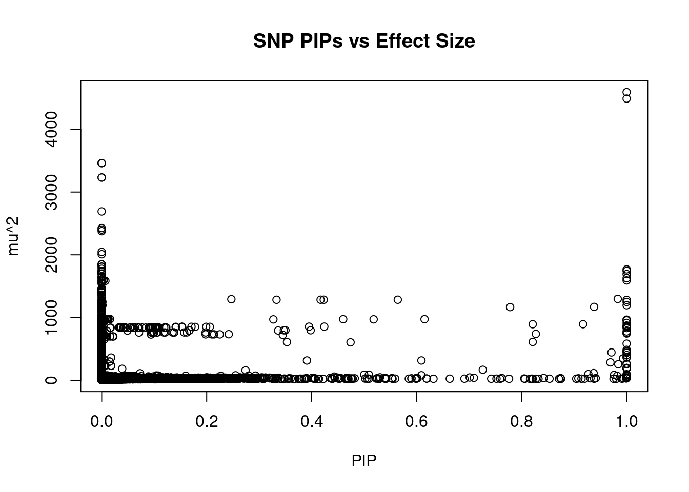
| Version | Author | Date |
|---|---|---|
| 3a7fbc1 | wesleycrouse | 2021-09-08 |
#SNPs with 50 largest effect sizes
head(ctwas_snp_res[order(-ctwas_snp_res$mu2),report_cols_snps],50)
id region_tag susie_pip mu2 PVE z
287582 rs2523507 6_25 1.000 4590.62 1.4e-02 6.84
287583 rs2239528 6_25 1.000 4488.64 1.3e-02 -6.84
287562 rs3093953 6_25 0.000 3461.41 0.0e+00 6.20
287559 rs2286713 6_25 0.000 3461.35 0.0e+00 6.20
287561 rs3093954 6_25 0.000 3461.35 0.0e+00 6.20
287576 rs3093979 6_25 0.000 3231.84 0.0e+00 5.97
287575 rs3093984 6_25 0.000 3231.63 0.0e+00 5.97
287541 rs9267293 6_25 0.000 2690.91 0.0e+00 6.07
287531 rs2905722 6_25 0.000 2425.95 0.0e+00 6.81
287521 rs2523670 6_25 0.000 2402.18 0.0e+00 6.83
287569 rs3094000 6_25 0.000 2376.32 0.0e+00 5.76
287558 rs28703977 6_25 0.000 2045.30 0.0e+00 5.94
287472 rs3132091 6_25 0.000 2008.72 0.0e+00 7.19
287589 rs2516391 6_25 0.000 1847.93 0.0e+00 6.59
287590 rs3094595 6_25 0.000 1847.84 0.0e+00 6.58
287591 rs928815 6_25 0.000 1847.13 0.0e+00 6.58
287106 rs9264024 6_25 0.000 1811.92 0.0e+00 6.59
287105 rs3130520 6_25 0.000 1808.43 0.0e+00 6.56
287356 rs2596488 6_25 0.000 1777.03 0.0e+00 6.95
288117 rs17612548 6_26 1.000 1768.33 5.3e-03 11.17
288138 rs3134996 6_26 1.000 1743.80 5.2e-03 10.37
287174 rs3134744 6_25 0.000 1738.84 0.0e+00 6.36
287167 rs28498059 6_25 0.000 1737.93 0.0e+00 6.35
287124 rs3130532 6_25 0.000 1733.88 0.0e+00 6.37
287129 rs3095246 6_25 0.000 1733.55 0.0e+00 6.36
287096 rs3130950 6_25 0.000 1730.94 0.0e+00 6.41
288116 rs17612510 6_26 0.000 1702.17 1.7e-08 10.42
288124 rs9273524 6_26 0.000 1696.69 0.0e+00 10.93
288118 rs17612633 6_26 0.000 1695.59 0.0e+00 10.90
288108 rs9272679 6_26 1.000 1692.31 5.0e-03 -9.31
288115 rs9273242 6_26 0.000 1691.70 0.0e+00 10.58
287353 rs2523605 6_25 0.000 1650.20 0.0e+00 4.99
287322 rs2508000 6_25 0.000 1640.54 0.0e+00 5.98
287552 rs2855807 6_25 0.000 1637.90 0.0e+00 5.27
287556 rs2534659 6_25 0.000 1637.88 0.0e+00 5.27
286537 rs34662244 6_22 1.000 1627.88 4.8e-03 4.07
287272 rs9264970 6_25 0.000 1603.16 0.0e+00 6.08
286592 rs13191786 6_22 0.004 1595.71 1.9e-05 4.10
286595 rs34218844 6_22 0.003 1595.46 1.6e-05 4.09
286555 rs67297533 6_22 1.000 1591.93 4.7e-03 -4.09
286581 rs67998226 6_22 0.007 1585.02 3.1e-05 4.25
286600 rs35030260 6_22 0.000 1583.36 2.2e-06 4.12
286586 rs33932084 6_22 0.000 1578.19 2.2e-08 3.93
286605 rs13198809 6_22 0.000 1556.78 3.2e-09 4.08
286614 rs36092177 6_22 0.000 1549.62 6.3e-10 4.08
286639 rs55690788 6_22 0.000 1542.13 5.4e-10 4.16
287190 rs7381988 6_25 0.000 1463.97 0.0e+00 6.06
287485 rs3130483 6_25 0.000 1462.60 0.0e+00 5.36
287429 rs2596517 6_25 0.000 1460.52 0.0e+00 6.78
286751 rs1311917 6_22 0.000 1458.82 0.0e+00 3.82SNPs with highest PVE
#SNPs with 50 highest pve
head(ctwas_snp_res[order(-ctwas_snp_res$PVE),report_cols_snps],50)
id region_tag susie_pip mu2 PVE z
287582 rs2523507 6_25 1.000 4590.62 0.01400 6.84
287583 rs2239528 6_25 1.000 4488.64 0.01300 -6.84
288117 rs17612548 6_26 1.000 1768.33 0.00530 11.17
288138 rs3134996 6_26 1.000 1743.80 0.00520 10.37
288108 rs9272679 6_26 1.000 1692.31 0.00500 -9.31
286537 rs34662244 6_22 1.000 1627.88 0.00480 4.07
286555 rs67297533 6_22 1.000 1591.93 0.00470 -4.09
719600 rs2064505 20_20 1.000 1281.35 0.00380 -3.92
769930 rs3129696 6_24 0.983 1297.54 0.00380 -3.92
719599 rs2747568 20_20 1.000 1249.50 0.00370 3.79
406861 rs16902104 8_83 1.000 1196.48 0.00360 3.51
406860 rs16902103 8_83 0.938 1170.16 0.00330 -3.50
471145 rs2019640 10_59 1.000 963.44 0.00290 -3.47
471147 rs913647 10_59 1.000 965.88 0.00290 3.45
209719 rs2125449 4_79 1.000 954.96 0.00280 -3.33
169901 rs28661518 3_112 1.000 915.31 0.00270 -3.09
406858 rs34585331 8_83 0.778 1166.53 0.00270 -3.55
82161 rs12471681 2_53 1.000 873.56 0.00260 -3.05
790569 rs2939608 12_56 1.000 859.88 0.00260 -2.96
486071 rs11041828 11_6 1.000 833.29 0.00250 2.96
486072 rs4237770 11_6 1.000 851.82 0.00250 -2.93
169902 rs73190822 3_112 0.917 894.42 0.00240 3.11
252840 rs3910018 5_51 1.000 778.84 0.00230 -2.86
37018 rs75222047 1_85 1.000 755.36 0.00220 2.91
42580 rs2776714 1_97 1.000 745.72 0.00220 -2.78
169900 rs62287225 3_112 0.821 894.19 0.00220 3.08
769877 rs2844773 6_24 0.564 1284.36 0.00220 3.95
37037 rs2179109 1_85 0.827 739.23 0.00180 -3.03
209739 rs11721784 4_79 0.615 973.76 0.00180 3.38
139434 rs13062973 3_45 1.000 584.80 0.00170 -3.60
769894 rs2188099 6_24 0.417 1284.10 0.00160 3.92
769898 rs2844770 6_24 0.423 1284.11 0.00160 3.92
139422 rs34695932 3_45 0.821 611.97 0.00150 4.13
209705 rs13109930 4_79 0.518 971.58 0.00150 3.11
167435 rs1388475 3_107 1.000 485.85 0.00140 2.87
167436 rs13071192 3_107 1.000 463.91 0.00140 -3.12
498342 rs11603701 11_30 1.000 455.08 0.00140 -3.24
167438 rs13081434 3_107 0.971 444.68 0.00130 -2.47
209726 rs1542437 4_79 0.460 974.07 0.00130 3.35
498011 rs113527193 11_30 1.000 437.47 0.00130 3.29
769882 rs2844771 6_24 0.333 1283.67 0.00130 3.91
378881 rs1495743 8_21 1.000 401.73 0.00120 3.21
82157 rs75755471 2_53 0.424 855.33 0.00110 3.07
435734 rs7025746 9_53 1.000 369.30 0.00110 -3.04
435738 rs2900388 9_53 1.000 362.42 0.00110 3.51
82163 rs78406274 2_53 0.395 855.21 0.00100 3.06
378884 rs34537991 8_21 0.993 347.66 0.00100 3.06
769922 rs2022083 6_24 0.247 1292.31 0.00095 -3.89
209707 rs6819187 4_79 0.327 970.88 0.00094 3.09
252851 rs10805847 5_51 0.398 797.05 0.00094 2.87SNPs with largest z scores
#SNPs with 50 largest z scores
head(ctwas_snp_res[order(-abs(ctwas_snp_res$z)),report_cols_snps],50)
id region_tag susie_pip mu2 PVE z
476508 rs12260037 10_70 0.006 227.55 4.1e-06 22.65
476500 rs12244851 10_70 1.000 255.37 7.6e-04 22.39
476497 rs6585198 10_70 0.001 127.05 5.3e-07 15.56
476509 rs12359102 10_70 0.001 97.23 2.1e-07 14.81
476507 rs7077039 10_70 0.001 96.97 2.1e-07 14.79
476505 rs7921525 10_70 0.001 93.64 2.1e-07 14.58
476513 rs4077527 10_70 0.001 88.10 2.0e-07 14.57
476506 rs6585203 10_70 0.001 92.73 2.1e-07 14.52
476502 rs11196191 10_70 0.001 92.54 2.1e-07 14.51
476503 rs10787472 10_70 0.001 92.11 2.1e-07 14.49
288160 rs9275221 6_26 0.000 351.54 0.0e+00 12.84
288211 rs9275583 6_26 0.000 351.65 0.0e+00 12.83
288168 rs9275275 6_26 0.000 350.12 0.0e+00 12.82
288173 rs9275307 6_26 0.000 350.40 0.0e+00 12.82
288204 rs4273728 6_26 0.000 350.47 0.0e+00 12.82
288162 rs9275223 6_26 0.000 349.94 0.0e+00 12.81
288119 rs17612712 6_26 0.000 1215.14 0.0e+00 12.39
476491 rs12243578 10_70 0.003 80.66 6.5e-07 12.36
288180 rs9275362 6_26 0.000 181.30 0.0e+00 11.83
288121 rs9273354 6_26 0.000 1146.57 0.0e+00 11.78
288117 rs17612548 6_26 1.000 1768.33 5.3e-03 11.17
288040 rs617578 6_26 0.000 257.59 0.0e+00 11.10
288124 rs9273524 6_26 0.000 1696.69 0.0e+00 10.93
288118 rs17612633 6_26 0.000 1695.59 0.0e+00 10.90
288136 rs3828800 6_26 0.000 270.18 0.0e+00 10.83
288125 rs9273528 6_26 0.000 237.12 0.0e+00 10.73
288222 rs3916765 6_27 1.000 97.35 2.9e-04 10.72
288109 rs34763586 6_26 0.000 441.71 0.0e+00 10.63
288127 rs28724252 6_26 0.000 234.12 0.0e+00 10.61
288115 rs9273242 6_26 0.000 1691.70 0.0e+00 10.58
288028 rs2760985 6_26 0.000 415.44 0.0e+00 10.56
170480 rs11929397 3_114 0.509 90.30 1.4e-04 10.55
170481 rs11716713 3_114 0.500 90.25 1.3e-04 10.55
288034 rs2647066 6_26 0.000 414.94 0.0e+00 10.52
288183 rs3135002 6_26 0.000 1019.38 0.0e+00 10.51
288053 rs3997872 6_26 0.000 415.86 0.0e+00 10.48
288116 rs17612510 6_26 0.000 1702.17 1.7e-08 10.42
288120 rs17612852 6_26 0.000 1229.92 0.0e+00 10.40
288138 rs3134996 6_26 1.000 1743.80 5.2e-03 10.37
284239 rs2206734 6_15 1.000 83.50 2.5e-04 10.34
288139 rs3134994 6_26 0.000 1128.19 0.0e+00 10.28
288133 rs3830058 6_26 0.000 1119.69 0.0e+00 10.17
288202 rs3129726 6_26 0.000 1086.56 0.0e+00 10.03
288179 rs3135190 6_26 0.000 1100.81 0.0e+00 9.99
785885 rs76895963 12_4 0.001 79.04 2.5e-07 -9.93
288013 rs12191360 6_26 0.000 445.06 0.0e+00 9.85
288106 rs41269945 6_26 0.000 434.20 0.0e+00 9.81
288064 rs3129757 6_26 0.000 745.07 0.0e+00 9.56
640888 rs79994966 16_29 0.293 74.92 6.5e-05 9.56
640884 rs17817712 16_29 0.280 74.79 6.2e-05 9.55Gene set enrichment for genes with PIP>0.8
#GO enrichment analysis
library(enrichR)
Welcome to enrichR
Checking connection ... Enrichr ... Connection is Live!
FlyEnrichr ... Connection is available!
WormEnrichr ... Connection is available!
YeastEnrichr ... Connection is available!
FishEnrichr ... Connection is available!dbs <- c("GO_Biological_Process_2021", "GO_Cellular_Component_2021", "GO_Molecular_Function_2021")
genes <- ctwas_gene_res$genename[ctwas_gene_res$susie_pip>0.8]
#number of genes for gene set enrichment
length(genes)[1] 4if (length(genes)>0){
GO_enrichment <- enrichr(genes, dbs)
for (db in dbs){
print(db)
df <- GO_enrichment[[db]]
df <- df[df$Adjusted.P.value<0.05,c("Term", "Overlap", "Adjusted.P.value", "Genes")]
print(df)
}
#DisGeNET enrichment
# devtools::install_bitbucket("ibi_group/disgenet2r")
library(disgenet2r)
disgenet_api_key <- get_disgenet_api_key(
email = "wesleycrouse@gmail.com",
password = "uchicago1" )
Sys.setenv(DISGENET_API_KEY= disgenet_api_key)
res_enrich <-disease_enrichment(entities=genes, vocabulary = "HGNC",
database = "CURATED" )
df <- res_enrich@qresult[1:10, c("Description", "FDR", "Ratio", "BgRatio")]
print(df)
#WebGestalt enrichment
library(WebGestaltR)
background <- ctwas_gene_res$genename
#listGeneSet()
databases <- c("pathway_KEGG", "disease_GLAD4U", "disease_OMIM")
enrichResult <- WebGestaltR(enrichMethod="ORA", organism="hsapiens",
interestGene=genes, referenceGene=background,
enrichDatabase=databases, interestGeneType="genesymbol",
referenceGeneType="genesymbol", isOutput=F)
print(enrichResult[,c("description", "size", "overlap", "FDR", "database", "userId")])
}Uploading data to Enrichr... Done.
Querying GO_Biological_Process_2021... Done.
Querying GO_Cellular_Component_2021... Done.
Querying GO_Molecular_Function_2021... Done.
Parsing results... Done.
[1] "GO_Biological_Process_2021"
Term
1 positive regulation of cyclin-dependent protein serine/threonine kinase activity (GO:0045737)
2 positive regulation of cyclin-dependent protein kinase activity (GO:1904031)
3 positive regulation of G1/S transition of mitotic cell cycle (GO:1900087)
4 positive regulation of cell cycle G1/S phase transition (GO:1902808)
5 regulation of cyclin-dependent protein kinase activity (GO:1904029)
6 positive regulation of mitotic cell cycle phase transition (GO:1901992)
7 positive regulation of cell cycle (GO:0045787)
8 regulation of G1/S transition of mitotic cell cycle (GO:2000045)
9 negative regulation of blood vessel morphogenesis (GO:2000181)
10 regulation of cyclin-dependent protein serine/threonine kinase activity (GO:0000079)
11 negative regulation of angiogenesis (GO:0016525)
12 positive regulation of protein serine/threonine kinase activity (GO:0071902)
13 regulation of protein serine/threonine kinase activity (GO:0071900)
Overlap Adjusted.P.value Genes
1 1/17 0.04557730 CCND2
2 1/20 0.04557730 CCND2
3 1/26 0.04557730 CCND2
4 1/35 0.04557730 CCND2
5 1/54 0.04557730 CCND2
6 1/58 0.04557730 CCND2
7 1/66 0.04557730 CCND2
8 1/71 0.04557730 CCND2
9 1/78 0.04557730 GTF2I
10 1/82 0.04557730 CCND2
11 1/87 0.04557730 GTF2I
12 1/106 0.04911562 CCND2
13 1/111 0.04911562 CCND2
[1] "GO_Cellular_Component_2021"
Term Overlap
1 cyclin-dependent protein kinase holoenzyme complex (GO:0000307) 1/30
2 serine/threonine protein kinase complex (GO:1902554) 1/37
Adjusted.P.value Genes
1 0.02951983 CCND2
2 0.02951983 CCND2
[1] "GO_Molecular_Function_2021"
[1] Term Overlap Adjusted.P.value Genes
<0 rows> (or 0-length row.names)XXbac-BPG13B8.10 gene(s) from the input list not found in DisGeNET CURATED Description FDR Ratio BgRatio
7 Communicating Hydrocephalus 0.005767842 1/3 7/9703
8 Diabetes Mellitus, Non-Insulin-Dependent 0.005767842 2/3 221/9703
13 Congenital Hydrocephalus 0.005767842 1/3 8/9703
14 Leukemia, Myelocytic, Acute 0.005767842 2/3 173/9703
17 Acute Myeloid Leukemia, M1 0.005767842 2/3 125/9703
23 Williams Syndrome 0.005767842 1/3 8/9703
24 Endometrial Stromal Sarcoma 0.005767842 1/3 5/9703
25 POLYDACTYLY, POSTAXIAL 0.005767842 1/3 4/9703
30 Hydrocephalus Ex-Vacuo 0.005767842 1/3 7/9703
33 Post-Traumatic Hydrocephalus 0.005767842 1/3 7/9703******************************************
* *
* Welcome to WebGestaltR ! *
* *
******************************************Loading the functional categories...
Loading the ID list...
Loading the reference list...
Performing the enrichment analysis...
description size overlap FDR database
1 Chromosome Aberrations 175 3 0.01771986 disease_GLAD4U
userId
1 JAZF1;GTF2I;CCND2Sensitivity, specificity and precision for silver standard genes
library("readxl")

known_annotations <- read_xlsx("data/summary_known_genes_annotations.xlsx", sheet="T2D")
known_annotations <- unique(known_annotations$`Gene Symbol`)

unrelated_genes <- ctwas_gene_res$genename[!(ctwas_gene_res$genename %in% known_annotations)]

#number of genes in known annotations
print(length(known_annotations))
[1] 72#number of genes in known annotations with imputed expression
print(sum(known_annotations %in% ctwas_gene_res$genename))[1] 33#assign ctwas, TWAS, and bystander genes
ctwas_genes <- ctwas_gene_res$genename[ctwas_gene_res$susie_pip>0.8]
twas_genes <- ctwas_gene_res$genename[abs(ctwas_gene_res$z)>sig_thresh]
novel_genes <- ctwas_genes[!(ctwas_genes %in% twas_genes)]
#significance threshold for TWAS
print(sig_thresh)[1] 4.606075#number of ctwas genes
length(ctwas_genes)[1] 4#number of TWAS genes
length(twas_genes)[1] 42#show novel genes (ctwas genes with not in TWAS genes)
ctwas_gene_res[ctwas_gene_res$genename %in% novel_genes,report_cols][1] genename region_tag susie_pip mu2 PVE z
<0 rows> (or 0-length row.names)#sensitivity / recall
sensitivity <- rep(NA,2)
names(sensitivity) <- c("ctwas", "TWAS")
sensitivity["ctwas"] <- sum(ctwas_genes %in% known_annotations)/length(known_annotations)
sensitivity["TWAS"] <- sum(twas_genes %in% known_annotations)/length(known_annotations)
sensitivity ctwas TWAS
0.00000000 0.02777778 #specificity
specificity <- rep(NA,2)
names(specificity) <- c("ctwas", "TWAS")
specificity["ctwas"] <- sum(!(unrelated_genes %in% ctwas_genes))/length(unrelated_genes)
specificity["TWAS"] <- sum(!(unrelated_genes %in% twas_genes))/length(unrelated_genes)
specificity ctwas TWAS
0.9996708 0.9967084 #precision / PPV
precision <- rep(NA,2)
names(precision) <- c("ctwas", "TWAS")
precision["ctwas"] <- sum(ctwas_genes %in% known_annotations)/length(ctwas_genes)
precision["TWAS"] <- sum(twas_genes %in% known_annotations)/length(twas_genes)
precision ctwas TWAS
0.00000000 0.04761905 #ROC curves
pip_range <- (0:1000)/1000
sensitivity <- rep(NA, length(pip_range))
specificity <- rep(NA, length(pip_range))
for (index in 1:length(pip_range)){
pip <- pip_range[index]
ctwas_genes <- ctwas_gene_res$genename[ctwas_gene_res$susie_pip>=pip]
sensitivity[index] <- sum(ctwas_genes %in% known_annotations)/length(known_annotations)
specificity[index] <- sum(!(unrelated_genes %in% ctwas_genes))/length(unrelated_genes)
}
plot(1-specificity, sensitivity, type="l", xlim=c(0,1), ylim=c(0,1))
sig_thresh_range <- seq(from=0, to=max(abs(ctwas_gene_res$z)), length.out=length(pip_range))
for (index in 1:length(sig_thresh_range)){
sig_thresh_plot <- sig_thresh_range[index]
twas_genes <- ctwas_gene_res$genename[abs(ctwas_gene_res$z)>=sig_thresh_plot]
sensitivity[index] <- sum(twas_genes %in% known_annotations)/length(known_annotations)
specificity[index] <- sum(!(unrelated_genes %in% twas_genes))/length(unrelated_genes)
}
lines(1-specificity, sensitivity, xlim=c(0,1), ylim=c(0,1), col="red", lty=2)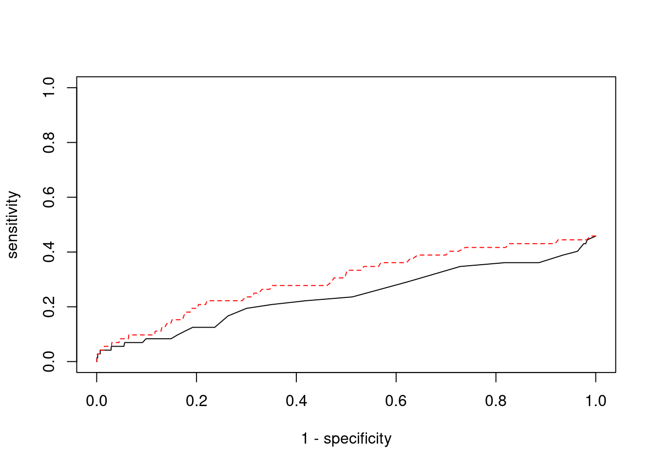
| Version | Author | Date |
|---|---|---|
| 3a7fbc1 | wesleycrouse | 2021-09-08 |
Sensitivity, specificity and precision for silver standard genes - bystanders only
This section first uses all silver standard genes to identify bystander genes within 1Mb. The silver standard and bystander gene lists are then subset to only genes with imputed expression in this analysis. Then, the ctwas and TWAS gene lists from this analysis are subset to only genes that are in the (subset) silver standard and bystander genes. These gene lists are then used to compute sensitivity, specificity and precision for ctwas and TWAS.
library(biomaRt)
library(GenomicRanges)Loading required package: stats4Loading required package: BiocGenericsLoading required package: parallel
Attaching package: 'BiocGenerics'The following objects are masked from 'package:parallel':
clusterApply, clusterApplyLB, clusterCall, clusterEvalQ,
clusterExport, clusterMap, parApply, parCapply, parLapply,
parLapplyLB, parRapply, parSapply, parSapplyLBThe following objects are masked from 'package:stats':
IQR, mad, sd, var, xtabsThe following objects are masked from 'package:base':
anyDuplicated, append, as.data.frame, basename, cbind,
colnames, dirname, do.call, duplicated, eval, evalq, Filter,
Find, get, grep, grepl, intersect, is.unsorted, lapply, Map,
mapply, match, mget, order, paste, pmax, pmax.int, pmin,
pmin.int, Position, rank, rbind, Reduce, rownames, sapply,
setdiff, sort, table, tapply, union, unique, unsplit, which,
which.max, which.minLoading required package: S4Vectors
Attaching package: 'S4Vectors'The following object is masked from 'package:base':
expand.gridLoading required package: IRangesLoading required package: GenomeInfoDbensembl <- useEnsembl(biomart="ENSEMBL_MART_ENSEMBL", dataset="hsapiens_gene_ensembl")
G_list <- getBM(filters= "chromosome_name", attributes= c("hgnc_symbol","chromosome_name","start_position","end_position","gene_biotype"), values=1:22, mart=ensembl)
G_list <- G_list[G_list$hgnc_symbol!="",]
G_list <- G_list[G_list$gene_biotype %in% c("protein_coding","lncRNA"),]
G_list$start <- G_list$start_position
G_list$end <- G_list$end_position
G_list_granges <- makeGRangesFromDataFrame(G_list, keep.extra.columns=T)
known_annotations_positions <- G_list[G_list$hgnc_symbol %in% known_annotations,]
half_window <- 1000000
known_annotations_positions$start <- known_annotations_positions$start_position - half_window
known_annotations_positions$end <- known_annotations_positions$end_position + half_window
known_annotations_positions$start[known_annotations_positions$start<1] <- 1
known_annotations_granges <- makeGRangesFromDataFrame(known_annotations_positions, keep.extra.columns=T)
bystanders <- findOverlaps(known_annotations_granges,G_list_granges)
bystanders <- unique(subjectHits(bystanders))
bystanders <- G_list$hgnc_symbol[bystanders]
bystanders <- bystanders[!(bystanders %in% known_annotations)]
unrelated_genes <- bystanders
#number of genes in known annotations
print(length(known_annotations))[1] 72#number of genes in known annotations with imputed expression
print(sum(known_annotations %in% ctwas_gene_res$genename))[1] 33#number of bystander genes
print(length(unrelated_genes))[1] 1837#number of bystander genes with imputed expression
print(sum(unrelated_genes %in% ctwas_gene_res$genename))[1] 949#remove genes without imputed expression from gene lists
known_annotations <- known_annotations[known_annotations %in% ctwas_gene_res$genename]
unrelated_genes <- unrelated_genes[unrelated_genes %in% ctwas_gene_res$genename]
#assign ctwas and TWAS genes
ctwas_genes <- ctwas_gene_res$genename[ctwas_gene_res$susie_pip>0.8]
twas_genes <- ctwas_gene_res$genename[abs(ctwas_gene_res$z)>sig_thresh]
#significance threshold for TWAS
print(sig_thresh)[1] 4.606075#number of ctwas genes
length(ctwas_genes)[1] 4#number of ctwas genes in known annotations or bystanders
sum(ctwas_genes %in% c(known_annotations, unrelated_genes))[1] 0#number of ctwas genes
length(twas_genes)[1] 42#number of TWAS genes
sum(twas_genes %in% c(known_annotations, unrelated_genes))[1] 7#remove genes not in known or bystander lists from results
ctwas_genes <- ctwas_genes[ctwas_genes %in% c(known_annotations, unrelated_genes)]
twas_genes <- twas_genes[twas_genes %in% c(known_annotations, unrelated_genes)]
#sensitivity / recall
sensitivity <- rep(NA,2)
names(sensitivity) <- c("ctwas", "TWAS")
sensitivity["ctwas"] <- sum(ctwas_genes %in% known_annotations)/length(known_annotations)
sensitivity["TWAS"] <- sum(twas_genes %in% known_annotations)/length(known_annotations)
sensitivity
ctwas TWAS
0.00000000 0.06060606 #specificity
specificity <- rep(NA,2)
names(specificity) <- c("ctwas", "TWAS")
specificity["ctwas"] <- sum(!(unrelated_genes %in% ctwas_genes))/length(unrelated_genes)
specificity["TWAS"] <- sum(!(unrelated_genes %in% twas_genes))/length(unrelated_genes)
specificity ctwas TWAS
1.0000000 0.9947313 #precision / PPV
precision <- rep(NA,2)
names(precision) <- c("ctwas", "TWAS")
precision["ctwas"] <- sum(ctwas_genes %in% known_annotations)/length(ctwas_genes)
precision["TWAS"] <- sum(twas_genes %in% known_annotations)/length(twas_genes)
precision ctwas TWAS
NaN 0.2857143
sessionInfo()R version 3.6.1 (2019-07-05)
Platform: x86_64-pc-linux-gnu (64-bit)
Running under: Scientific Linux 7.4 (Nitrogen)
Matrix products: default
BLAS/LAPACK: /software/openblas-0.2.19-el7-x86_64/lib/libopenblas_haswellp-r0.2.19.so
locale:
[1] LC_CTYPE=en_US.UTF-8 LC_NUMERIC=C
[3] LC_TIME=en_US.UTF-8 LC_COLLATE=en_US.UTF-8
[5] LC_MONETARY=en_US.UTF-8 LC_MESSAGES=en_US.UTF-8
[7] LC_PAPER=en_US.UTF-8 LC_NAME=C
[9] LC_ADDRESS=C LC_TELEPHONE=C
[11] LC_MEASUREMENT=en_US.UTF-8 LC_IDENTIFICATION=C
attached base packages:
[1] parallel stats4 stats graphics grDevices utils datasets
[8] methods base
other attached packages:
[1] GenomicRanges_1.36.0 GenomeInfoDb_1.20.0 IRanges_2.18.1
[4] S4Vectors_0.22.1 BiocGenerics_0.30.0 biomaRt_2.40.1
[7] readxl_1.3.1 WebGestaltR_0.4.4 disgenet2r_0.99.2
[10] enrichR_3.0 cowplot_1.0.0 ggplot2_3.3.3
loaded via a namespace (and not attached):
[1] bitops_1.0-6 fs_1.3.1 bit64_4.0.5
[4] doParallel_1.0.16 progress_1.2.2 httr_1.4.1
[7] rprojroot_2.0.2 tools_3.6.1 doRNG_1.8.2
[10] utf8_1.2.1 R6_2.5.0 DBI_1.1.1
[13] colorspace_1.4-1 withr_2.4.1 tidyselect_1.1.0
[16] prettyunits_1.0.2 bit_4.0.4 curl_3.3
[19] compiler_3.6.1 git2r_0.26.1 Biobase_2.44.0
[22] labeling_0.3 scales_1.1.0 readr_1.4.0
[25] stringr_1.4.0 apcluster_1.4.8 digest_0.6.20
[28] rmarkdown_1.13 svglite_1.2.2 XVector_0.24.0
[31] pkgconfig_2.0.3 htmltools_0.3.6 fastmap_1.1.0
[34] rlang_0.4.11 RSQLite_2.2.7 farver_2.1.0
[37] generics_0.0.2 jsonlite_1.6 dplyr_1.0.7
[40] RCurl_1.98-1.1 magrittr_2.0.1 GenomeInfoDbData_1.2.1
[43] Matrix_1.2-18 Rcpp_1.0.6 munsell_0.5.0
[46] fansi_0.5.0 gdtools_0.1.9 lifecycle_1.0.0
[49] stringi_1.4.3 whisker_0.3-2 yaml_2.2.0
[52] zlibbioc_1.30.0 plyr_1.8.4 grid_3.6.1
[55] blob_1.2.1 promises_1.0.1 crayon_1.4.1
[58] lattice_0.20-38 hms_1.1.0 knitr_1.23
[61] pillar_1.6.1 igraph_1.2.4.1 rjson_0.2.20
[64] rngtools_1.5 reshape2_1.4.3 codetools_0.2-16
[67] XML_3.98-1.20 glue_1.4.2 evaluate_0.14
[70] data.table_1.14.0 vctrs_0.3.8 httpuv_1.5.1
[73] foreach_1.5.1 cellranger_1.1.0 gtable_0.3.0
[76] purrr_0.3.4 assertthat_0.2.1 cachem_1.0.5
[79] xfun_0.8 later_0.8.0 tibble_3.1.2
[82] iterators_1.0.13 AnnotationDbi_1.46.0 memoise_2.0.0
[85] workflowr_1.6.2 ellipsis_0.3.2