Diabetes diagnosed by doctor - Adipose

Last updated: 2021-09-13

Checks: 7 0

Knit directory: ctwas_applied/

This reproducible R Markdown analysis was created with workflowr (version 1.6.2). The Checks tab describes the reproducibility checks that were applied when the results were created. The Past versions tab lists the development history.

R Markdown file: up-to-date

Great! Since the R Markdown file has been committed to the Git repository, you know the exact version of the code that produced these results.

Environment: empty

Great job! The global environment was empty. Objects defined in the global environment can affect the analysis in your R Markdown file in unknown ways. For reproduciblity it’s best to always run the code in an empty environment.

Seed: set.seed(20210726)

The command set.seed(20210726) was run prior to running the code in the R Markdown file. Setting a seed ensures that any results that rely on randomness, e.g. subsampling or permutations, are reproducible.

Session information: recorded

Great job! Recording the operating system, R version, and package versions is critical for reproducibility.

Cache: none

Nice! There were no cached chunks for this analysis, so you can be confident that you successfully produced the results during this run.

File paths: relative

Great job! Using relative paths to the files within your workflowr project makes it easier to run your code on other machines.

Repository version: 72c8ef7

Great! You are using Git for version control. Tracking code development and connecting the code version to the results is critical for reproducibility.

The results in this page were generated with repository version 72c8ef7. See the Past versions tab to see a history of the changes made to the R Markdown and HTML files.

Note that you need to be careful to ensure that all relevant files for the analysis have been committed to Git prior to generating the results (you can use wflow_publish or wflow_git_commit). workflowr only checks the R Markdown file, but you know if there are other scripts or data files that it depends on. Below is the status of the Git repository when the results were generated:


working directory clean

Note that any generated files, e.g. HTML, png, CSS, etc., are not included in this status report because it is ok for generated content to have uncommitted changes.

These are the previous versions of the repository in which changes were made to the R Markdown (analysis/ukb-a-306_Adipose_Subcutaneous_known.Rmd) and HTML (docs/ukb-a-306_Adipose_Subcutaneous_known.html) files. If you’ve configured a remote Git repository (see ?wflow_git_remote), click on the hyperlinks in the table below to view the files as they were in that past version.

File	Version	Author	Date	Message
Rmd	72c8ef7	wesleycrouse	2021-09-13	changing mart for biomart
Rmd	a49c40e	wesleycrouse	2021-09-13	updating with bystander analysis
html	7e22565	wesleycrouse	2021-09-13	updating reports
html	3a7fbc1	wesleycrouse	2021-09-08	generating reports for known annotations
Rmd	cbf7408	wesleycrouse	2021-09-08	adding enrichment to reports

Overview

These are the results of a ctwas analysis of the UK Biobank trait Diabetes diagnosed by doctor using Adipose_Subcutaneous gene weights.

The GWAS was conducted by the Neale Lab, and the biomarker traits we analyzed are discussed here. Summary statistics were obtained from IEU OpenGWAS using GWAS ID: ukb-a-306. Results were obtained from from IEU rather than Neale Lab because they are in a standardard format (GWAS VCF). Note that 3 of the 34 biomarker traits were not available from IEU and were excluded from analysis.

The weights are mashr GTEx v8 models on Adipose_Subcutaneous eQTL obtained from PredictDB. We performed a full harmonization of the variants, including recovering strand ambiguous variants. This procedure is discussed in a separate document. (TO-DO: add report that describes harmonization)

LD matrices were computed from a 10% subset of Neale lab subjects. Subjects were matched using the plate and well information from genotyping. We included only biallelic variants with MAF>0.01 in the original Neale Lab GWAS. (TO-DO: add more details [number of subjects, variants, etc])

Weight QC

TO-DO: add enhanced QC reporting (total number of weights, why each variant was missing for all genes)

qclist_all <- list()

qc_files <- paste0(results_dir, "/", list.files(results_dir, pattern="exprqc.Rd"))

for (i in 1:length(qc_files)){
  load(qc_files[i])
  chr <- unlist(strsplit(rev(unlist(strsplit(qc_files[i], "_")))[1], "[.]"))[1]
  qclist_all[[chr]] <- cbind(do.call(rbind, lapply(qclist,unlist)), as.numeric(substring(chr,4)))
}

qclist_all <- data.frame(do.call(rbind, qclist_all))
colnames(qclist_all)[ncol(qclist_all)] <- "chr"

rm(qclist, wgtlist, z_gene_chr)

#number of imputed weights
nrow(qclist_all)

[1] 12414

#number of imputed weights by chromosome
table(qclist_all$chr)


   1    2    3    4    5    6    7    8    9   10   11   12   13   14   15 
1223  885  712  493  574  708  607  468  472  481  750  671  248  411  431 
  16   17   18   19   20   21   22 
 580  758  186  940  370  138  308

#proportion of imputed weights without missing variants
mean(qclist_all$nmiss==0)

[1] 0.7137909

Load ctwas results

#load ctwas results
ctwas_res <- data.table::fread(paste0(results_dir, "/", analysis_id, "_ctwas.susieIrss.txt"))

#make unique identifier for regions
ctwas_res$region_tag <- paste(ctwas_res$region_tag1, ctwas_res$region_tag2, sep="_")

#load z scores for SNPs and collect sample size
load(paste0(results_dir, "/", analysis_id, "_expr_z_snp.Rd"))

sample_size <- z_snp$ss
sample_size <- as.numeric(names(which.max(table(sample_size))))

#compute PVE for each gene/SNP
ctwas_res$PVE = ctwas_res$susie_pip*ctwas_res$mu2/sample_size

#separate gene and SNP results
ctwas_gene_res <- ctwas_res[ctwas_res$type == "gene", ]
ctwas_gene_res <- data.frame(ctwas_gene_res)
ctwas_snp_res <- ctwas_res[ctwas_res$type == "SNP", ]
ctwas_snp_res <- data.frame(ctwas_snp_res)

#add gene information to results
sqlite <- RSQLite::dbDriver("SQLite")
db = RSQLite::dbConnect(sqlite, paste0("/project2/compbio/predictdb/mashr_models/mashr_", weight, ".db"))
query <- function(...) RSQLite::dbGetQuery(db, ...)
gene_info <- query("select gene, genename from extra")
gene_info <- query("select gene, genename, gene_type from extra")
RSQLite::dbDisconnect(db)

ctwas_gene_res <- cbind(ctwas_gene_res, gene_info[sapply(ctwas_gene_res$id, match, gene_info$gene), c("genename", "gene_type")])

#add z scores to results
load(paste0(results_dir, "/", analysis_id, "_expr_z_gene.Rd"))
ctwas_gene_res$z <- z_gene[ctwas_gene_res$id,]$z

z_snp <- z_snp[z_snp$id %in% ctwas_snp_res$id,]
ctwas_snp_res$z <- z_snp$z[match(ctwas_snp_res$id, z_snp$id)]

#formatting and rounding for tables
ctwas_gene_res$z <- round(ctwas_gene_res$z,2)
ctwas_snp_res$z <- round(ctwas_snp_res$z,2)
ctwas_gene_res$susie_pip <- round(ctwas_gene_res$susie_pip,3)
ctwas_snp_res$susie_pip <- round(ctwas_snp_res$susie_pip,3)
ctwas_gene_res$mu2 <- round(ctwas_gene_res$mu2,2)
ctwas_snp_res$mu2 <- round(ctwas_snp_res$mu2,2)
ctwas_gene_res$PVE <- signif(ctwas_gene_res$PVE, 2)
ctwas_snp_res$PVE <- signif(ctwas_snp_res$PVE, 2)

#merge gene and snp results with added information
ctwas_snp_res$genename=NA
ctwas_snp_res$gene_type=NA

ctwas_res <- rbind(ctwas_gene_res,
                   ctwas_snp_res[,colnames(ctwas_gene_res)])

#store columns to report
report_cols <- colnames(ctwas_gene_res)[!(colnames(ctwas_gene_res) %in% c("type", "region_tag1", "region_tag2", "cs_index", "gene_type", "z_flag", "id", "chrom", "pos"))]
first_cols <- c("genename", "region_tag")
report_cols <- c(first_cols, report_cols[!(report_cols %in% first_cols)])

report_cols_snps <- c("id", report_cols[-1])

#get number of SNPs from s1 results; adjust for thin
ctwas_res_s1 <- data.table::fread(paste0(results_dir, "/", analysis_id, "_ctwas.s1.susieIrss.txt"))
n_snps <- sum(ctwas_res_s1$type=="SNP")/thin
rm(ctwas_res_s1)

Check convergence of parameters

library(ggplot2)
library(cowplot)


********************************************************

Note: As of version 1.0.0, cowplot does not change the

  default ggplot2 theme anymore. To recover the previous

  behavior, execute:
  theme_set(theme_cowplot())

********************************************************

load(paste0(results_dir, "/", analysis_id, "_ctwas.s2.susieIrssres.Rd"))
  
df <- data.frame(niter = rep(1:ncol(group_prior_rec), 2),
                 value = c(group_prior_rec[1,], group_prior_rec[2,]),
                 group = rep(c("Gene", "SNP"), each = ncol(group_prior_rec)))
df$group <- as.factor(df$group)

df$value[df$group=="SNP"] <- df$value[df$group=="SNP"]*thin #adjust parameter to account for thin argument

p_pi <- ggplot(df, aes(x=niter, y=value, group=group)) +
  geom_line(aes(color=group)) +
  geom_point(aes(color=group)) +
  xlab("Iteration") + ylab(bquote(pi)) +
  ggtitle("Prior mean") +
  theme_cowplot()

df <- data.frame(niter = rep(1:ncol(group_prior_var_rec), 2),
                 value = c(group_prior_var_rec[1,], group_prior_var_rec[2,]),
                 group = rep(c("Gene", "SNP"), each = ncol(group_prior_var_rec)))
df$group <- as.factor(df$group)
p_sigma2 <- ggplot(df, aes(x=niter, y=value, group=group)) +
  geom_line(aes(color=group)) +
  geom_point(aes(color=group)) +
  xlab("Iteration") + ylab(bquote(sigma^2)) +
  ggtitle("Prior variance") +
  theme_cowplot()

plot_grid(p_pi, p_sigma2)

Version	Author	Date
3a7fbc1	wesleycrouse	2021-09-08

#estimated group prior
estimated_group_prior <- group_prior_rec[,ncol(group_prior_rec)]
names(estimated_group_prior) <- c("gene", "snp")
estimated_group_prior["snp"] <- estimated_group_prior["snp"]*thin #adjust parameter to account for thin argument
print(estimated_group_prior)

        gene          snp 
0.0072273144 0.0002145499

#estimated group prior variance
estimated_group_prior_var <- group_prior_var_rec[,ncol(group_prior_var_rec)]
names(estimated_group_prior_var) <- c("gene", "snp")
print(estimated_group_prior_var)

     gene       snp 
10.406176  5.441692

#report sample size
print(sample_size)

[1] 336473

#report group size
group_size <- c(nrow(ctwas_gene_res), n_snps)
print(group_size)

[1]   12414 7535010

#estimated group PVE
estimated_group_pve <- estimated_group_prior_var*estimated_group_prior*group_size/sample_size #check PVE calculation
names(estimated_group_pve) <- c("gene", "snp")
print(estimated_group_pve)

       gene         snp 
0.002774787 0.026145432

#compare sum(PIP*mu2/sample_size) with above PVE calculation
c(sum(ctwas_gene_res$PVE),sum(ctwas_snp_res$PVE))

[1] 0.0150731 0.3780328

Genes with highest PIPs

#distribution of PIPs
hist(ctwas_gene_res$susie_pip, xlim=c(0,1), main="Distribution of Gene PIPs")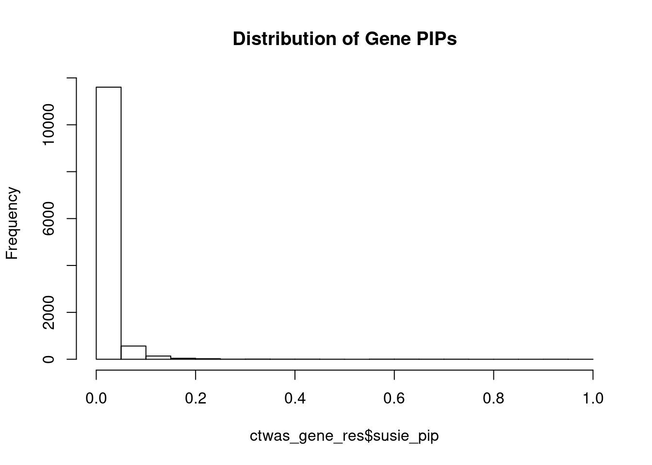

Version	Author	Date
3a7fbc1	wesleycrouse	2021-09-08

#genes with PIP>0.8 or 20 highest PIPs
head(ctwas_gene_res[order(-ctwas_gene_res$susie_pip),report_cols], max(sum(ctwas_gene_res$susie_pip>0.8), 20))

          genename region_tag susie_pip   mu2     PVE     z
3633         CCND2       12_4     0.998 92.56 2.7e-04  9.86
13893        GTF2I       7_48     0.938 27.22 7.6e-05 -5.11
7923         INHBB       2_70     0.902 22.20 5.9e-05 -4.47
356           ANK1       8_36     0.829 40.62 1.0e-04 -6.50
7067          NUS1       6_78     0.745 22.23 4.9e-05  4.44
7048         JAZF1       7_23     0.728 53.35 1.2e-04  7.66
1866       SLCO4A1      20_37     0.704 23.37 4.9e-05 -4.30
7749      C16orf59       16_2     0.696 23.77 4.9e-05 -3.88
152         TFAP2B       6_38     0.657 28.53 5.6e-05 -5.10
7109        LONRF1       8_15     0.655 25.77 5.0e-05  4.08
3647        CCDC92      12_75     0.649 25.81 5.0e-05  4.43
13258    LINC01184       5_78     0.647 21.34 4.1e-05 -4.05
11487        ZNF34       8_94     0.639 25.48 4.8e-05 -4.72
3200          SNX4       3_78     0.611 22.47 4.1e-05 -3.83
9518         MANEA       6_65     0.600 26.82 4.8e-05  3.99
2723          WFS1        4_7     0.596 63.57 1.1e-04 -8.28
14285 RP11-395N3.2      2_133     0.568 39.51 6.7e-05  6.44
3504         RAB29      1_104     0.563 21.24 3.6e-05  4.01
4222          OPA3      19_31     0.559 22.01 3.7e-05  3.96
5565         TACC2      10_76     0.521 25.32 3.9e-05  3.93

Genes with largest effect sizes

#plot PIP vs effect size
plot(ctwas_gene_res$susie_pip, ctwas_gene_res$mu2, xlab="PIP", ylab="mu^2", main="Gene PIPs vs Effect Size")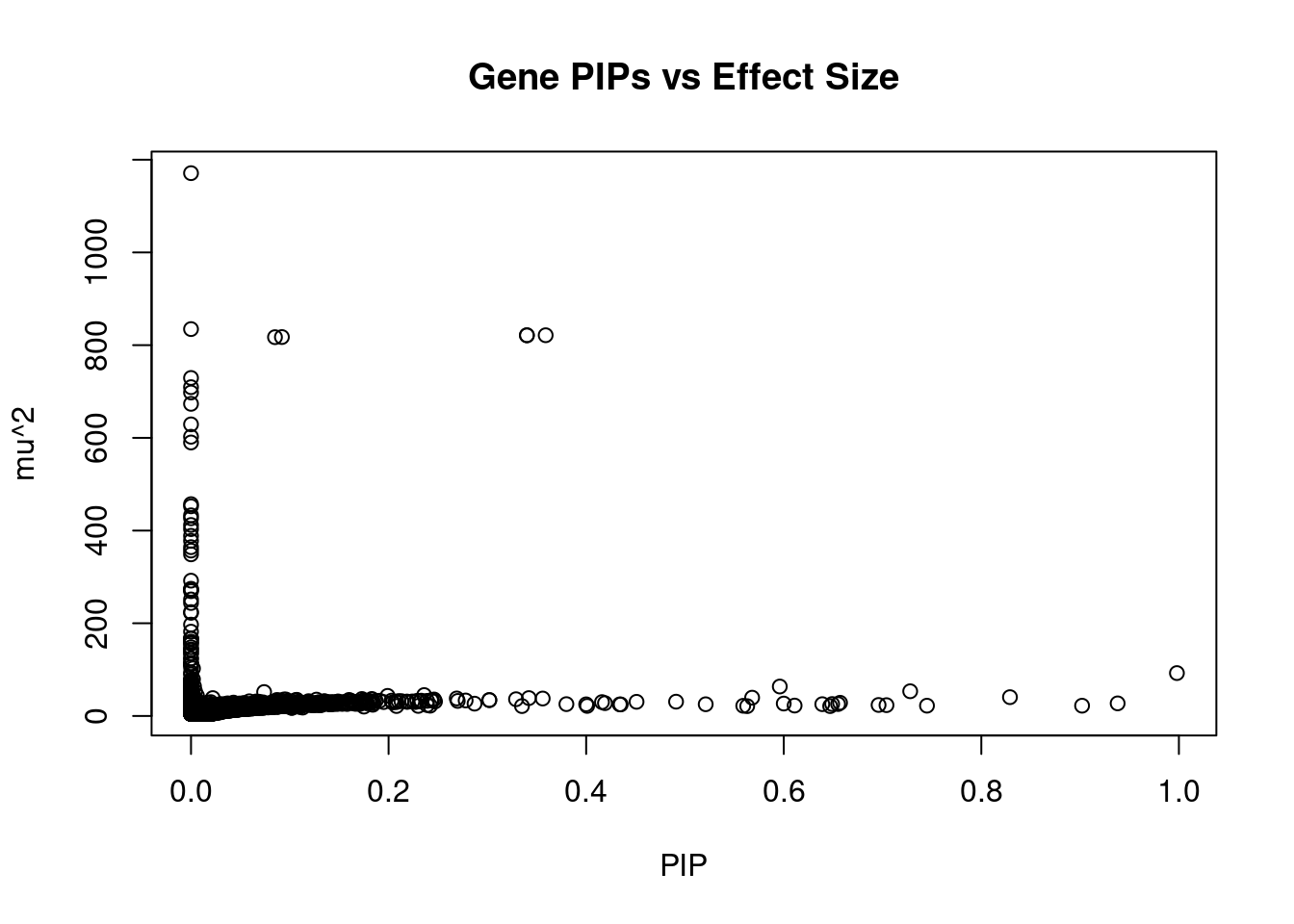

Version	Author	Date
3a7fbc1	wesleycrouse	2021-09-08

#genes with 20 largest effect sizes
head(ctwas_gene_res[order(-ctwas_gene_res$mu2),report_cols],20)

           genename region_tag susie_pip     mu2     PVE     z
6465        PPP1R18       6_24     0.000 1171.00 8.2e-15  5.18
12462     LINC00243       6_24     0.000  834.62 0.0e+00 -5.73
5257          THSD1      13_22     0.359  821.36 8.8e-04  2.37
5255          CKAP2      13_22     0.340  821.25 8.3e-04  2.37
14624 RP11-245D16.4      13_22     0.340  821.25 8.3e-04 -2.37
14412  RP11-93H24.3      13_22     0.092  817.45 2.2e-04 -2.33
8381          SUGT1      13_22     0.085  817.19 2.1e-04  2.33
13035      HLA-DQA2       6_26     0.000  729.22 0.0e+00 -9.41
11626          NEK5      13_22     0.000  709.34 9.3e-07 -2.22
12079          AGER       6_26     0.000  697.81 0.0e+00 -7.59
11608       ZSCAN26       6_22     0.000  673.37 0.0e+00  3.70
13457        UTP14C      13_22     0.000  629.07 1.6e-12 -1.56
8537             C2       6_26     0.000  602.40 0.0e+00 -8.14
11567       ZSCAN16       6_22     0.000  590.01 0.0e+00  2.16
5430          FLOT1       6_24     0.000  457.00 0.0e+00 -4.48
12080          RNF5       6_26     0.000  452.29 0.0e+00  6.17
12077        NOTCH4       6_26     0.000  432.86 0.0e+00  6.69
11407       ZKSCAN3       6_22     0.000  426.50 0.0e+00  2.62
12083         PRRT1       6_26     0.000  412.05 0.0e+00 -7.37
11236       ZSCAN23       6_22     0.000  403.10 0.0e+00 -2.34

Genes with highest PVE

#genes with 20 highest pve
head(ctwas_gene_res[order(-ctwas_gene_res$PVE),report_cols],20)

           genename region_tag susie_pip    mu2     PVE     z
5257          THSD1      13_22     0.359 821.36 8.8e-04  2.37
5255          CKAP2      13_22     0.340 821.25 8.3e-04  2.37
14624 RP11-245D16.4      13_22     0.340 821.25 8.3e-04 -2.37
3633          CCND2       12_4     0.998  92.56 2.7e-04  9.86
14412  RP11-93H24.3      13_22     0.092 817.45 2.2e-04 -2.33
8381          SUGT1      13_22     0.085 817.19 2.1e-04  2.33
7048          JAZF1       7_23     0.728  53.35 1.2e-04  7.66
2723           WFS1        4_7     0.596  63.57 1.1e-04 -8.28
356            ANK1       8_36     0.829  40.62 1.0e-04 -6.50
13893         GTF2I       7_48     0.938  27.22 7.6e-05 -5.11
14285  RP11-395N3.2      2_133     0.568  39.51 6.7e-05  6.44
7923          INHBB       2_70     0.902  22.20 5.9e-05 -4.47
152          TFAP2B       6_38     0.657  28.53 5.6e-05 -5.10
7109         LONRF1       8_15     0.655  25.77 5.0e-05  4.08
3647         CCDC92      12_75     0.649  25.81 5.0e-05  4.43
7067           NUS1       6_78     0.745  22.23 4.9e-05  4.44
7749       C16orf59       16_2     0.696  23.77 4.9e-05 -3.88
1866        SLCO4A1      20_37     0.704  23.37 4.9e-05 -4.30
9518          MANEA       6_65     0.600  26.82 4.8e-05  3.99
11487         ZNF34       8_94     0.639  25.48 4.8e-05 -4.72

Genes with largest z scores

#genes with 20 largest z scores
head(ctwas_gene_res[order(-abs(ctwas_gene_res$z)),report_cols],20)

          genename region_tag susie_pip    mu2     PVE     z
3633         CCND2       12_4     0.998  92.56 2.7e-04  9.86
13035     HLA-DQA2       6_26     0.000 729.22 0.0e+00 -9.41
2723          WFS1        4_7     0.596  63.57 1.1e-04 -8.28
8537            C2       6_26     0.000 602.40 0.0e+00 -8.14
7048         JAZF1       7_23     0.728  53.35 1.2e-04  7.66
12079         AGER       6_26     0.000 697.81 0.0e+00 -7.59
12097         NEU1       6_26     0.000 348.69 0.0e+00 -7.54
12083        PRRT1       6_26     0.000 412.05 0.0e+00 -7.37
12077       NOTCH4       6_26     0.000 432.86 0.0e+00  6.69
12371        CLIC1       6_26     0.000 364.16 0.0e+00  6.63
12101         VWA7       6_26     0.000 271.94 0.0e+00  6.54
12110         APOM       6_26     0.000 356.83 0.0e+00  6.52
356           ANK1       8_36     0.829  40.62 1.0e-04 -6.50
14285 RP11-395N3.2      2_133     0.568  39.51 6.7e-05  6.44
11430     HLA-DRB1       6_26     0.000 160.48 0.0e+00  6.44
12108       GPANK1       6_26     0.000 224.17 0.0e+00  6.37
12123       CCHCR1       6_26     0.000 167.14 0.0e+00 -6.25
12080         RNF5       6_26     0.000 452.29 0.0e+00  6.17
12075      HLA-DRA       6_26     0.000 251.42 0.0e+00 -5.97
12114         AIF1       6_26     0.000 273.21 0.0e+00 -5.93

Comparing z scores and PIPs

#set nominal signifiance threshold for z scores
alpha <- 0.05

#bonferroni adjusted threshold for z scores
sig_thresh <- qnorm(1-(alpha/nrow(ctwas_gene_res)/2), lower=T)

#Q-Q plot for z scores
obs_z <- ctwas_gene_res$z[order(ctwas_gene_res$z)]
exp_z <- qnorm((1:nrow(ctwas_gene_res))/nrow(ctwas_gene_res))

plot(exp_z, obs_z, xlab="Expected z", ylab="Observed z", main="Gene z score Q-Q plot")
abline(a=0,b=1)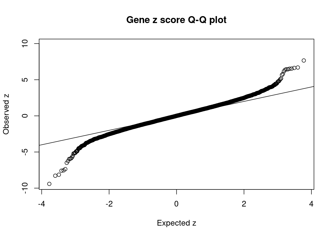

Version	Author	Date
3a7fbc1	wesleycrouse	2021-09-08

#plot z score vs PIP
plot(abs(ctwas_gene_res$z), ctwas_gene_res$susie_pip, xlab="abs(z)", ylab="PIP")
abline(v=sig_thresh, col="red", lty=2)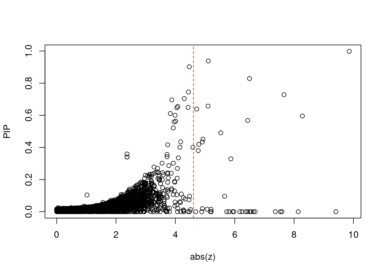

Version	Author	Date
3a7fbc1	wesleycrouse	2021-09-08

#proportion of significant z scores
mean(abs(ctwas_gene_res$z) > sig_thresh)

[1] 0.003141614

#genes with most significant z scores
head(ctwas_gene_res[order(-abs(ctwas_gene_res$z)),report_cols],20)

          genename region_tag susie_pip    mu2     PVE     z
3633         CCND2       12_4     0.998  92.56 2.7e-04  9.86
13035     HLA-DQA2       6_26     0.000 729.22 0.0e+00 -9.41
2723          WFS1        4_7     0.596  63.57 1.1e-04 -8.28
8537            C2       6_26     0.000 602.40 0.0e+00 -8.14
7048         JAZF1       7_23     0.728  53.35 1.2e-04  7.66
12079         AGER       6_26     0.000 697.81 0.0e+00 -7.59
12097         NEU1       6_26     0.000 348.69 0.0e+00 -7.54
12083        PRRT1       6_26     0.000 412.05 0.0e+00 -7.37
12077       NOTCH4       6_26     0.000 432.86 0.0e+00  6.69
12371        CLIC1       6_26     0.000 364.16 0.0e+00  6.63
12101         VWA7       6_26     0.000 271.94 0.0e+00  6.54
12110         APOM       6_26     0.000 356.83 0.0e+00  6.52
356           ANK1       8_36     0.829  40.62 1.0e-04 -6.50
14285 RP11-395N3.2      2_133     0.568  39.51 6.7e-05  6.44
11430     HLA-DRB1       6_26     0.000 160.48 0.0e+00  6.44
12108       GPANK1       6_26     0.000 224.17 0.0e+00  6.37
12123       CCHCR1       6_26     0.000 167.14 0.0e+00 -6.25
12080         RNF5       6_26     0.000 452.29 0.0e+00  6.17
12075      HLA-DRA       6_26     0.000 251.42 0.0e+00 -5.97
12114         AIF1       6_26     0.000 273.21 0.0e+00 -5.93

Locus plots for genes and SNPs

ctwas_gene_res_sortz <- ctwas_gene_res[order(-abs(ctwas_gene_res$z)),]

n_plots <- 5
for (region_tag_plot in head(unique(ctwas_gene_res_sortz$region_tag), n_plots)){
  ctwas_res_region <-  ctwas_res[ctwas_res$region_tag==region_tag_plot,]
  start <- min(ctwas_res_region$pos)
  end <- max(ctwas_res_region$pos)
  
  ctwas_res_region <- ctwas_res_region[order(ctwas_res_region$pos),]
  ctwas_res_region_gene <- ctwas_res_region[ctwas_res_region$type=="gene",]
  ctwas_res_region_snp <- ctwas_res_region[ctwas_res_region$type=="SNP",]
  
  #region name
  print(paste0("Region: ", region_tag_plot))
  
  #table of genes in region
  print(ctwas_res_region_gene[,report_cols])
  
  par(mfrow=c(4,1))
  
  #gene z scores
  plot(ctwas_res_region_gene$pos, abs(ctwas_res_region_gene$z), xlab="Position", ylab="abs(gene_z)", xlim=c(start,end),
   ylim=c(0,max(sig_thresh, abs(ctwas_res_region_gene$z))),
   main=paste0("Region: ", region_tag_plot))
  abline(h=sig_thresh,col="red",lty=2)
  
  #significance threshold for SNPs
  alpha_snp <- 5*10^(-8)
  sig_thresh_snp <- qnorm(1-alpha_snp/2, lower=T)
  
  #snp z scores
  plot(ctwas_res_region_snp$pos, abs(ctwas_res_region_snp$z), xlab="Position", ylab="abs(snp_z)",xlim=c(start,end),
   ylim=c(0,max(sig_thresh_snp, max(abs(ctwas_res_region_snp$z)))))
  abline(h=sig_thresh_snp,col="purple",lty=2)
  
  #gene pips
  plot(ctwas_res_region_gene$pos, ctwas_res_region_gene$susie_pip, xlab="Position", ylab="Gene PIP", xlim=c(start,end), ylim=c(0,1))
  abline(h=0.8,col="blue",lty=2)
  
  #snp pips
  plot(ctwas_res_region_snp$pos, ctwas_res_region_snp$susie_pip, xlab="Position", ylab="SNP PIP", xlim=c(start,end), ylim=c(0,1))
  abline(h=0.8,col="blue",lty=2)
}

[1] "Region: 12_4"
     genename region_tag susie_pip   mu2     PVE     z
4562  CRACR2A       12_4     0.016 13.85 6.7e-07  1.45
2871   PARP11       12_4     0.023 17.18 1.1e-06 -1.88
3633    CCND2       12_4     0.998 92.56 2.7e-04  9.86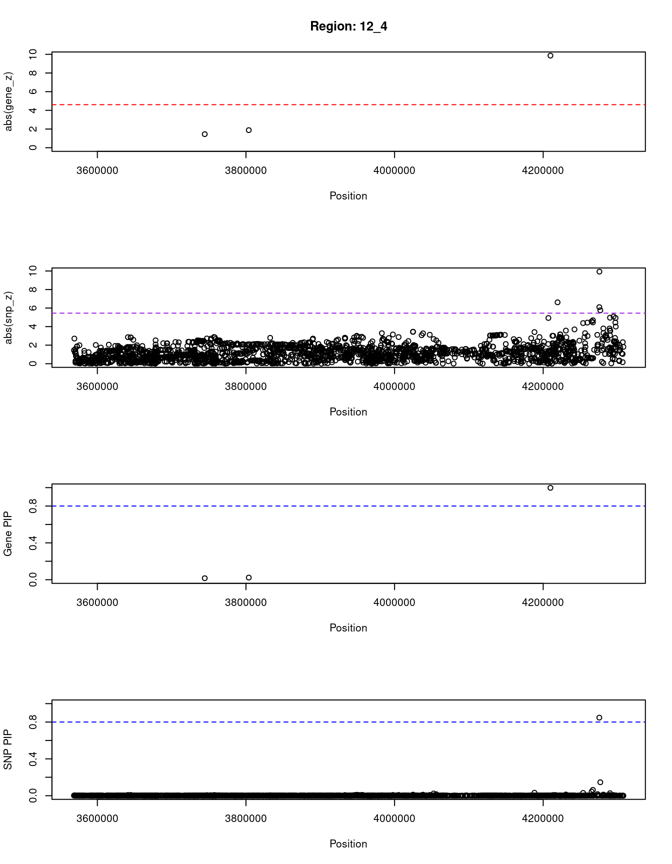

Version	Author	Date
3a7fbc1	wesleycrouse	2021-09-08

[1] "Region: 6_26"
               genename region_tag susie_pip    mu2 PVE     z
12132              DDR1       6_26         0  10.92   0 -1.24
11458             SFTA2       6_26         0  26.40   0  2.29
12376            GTF2H4       6_26         0   8.12   0  0.93
5440              VARS2       6_26         0   6.11   0  0.61
12753             HCG22       6_26         0  24.16   0  2.17
12122            POU5F1       6_26         0  21.85   0 -2.04
12125          PSORS1C1       6_26         0   4.69   0  0.18
12124          PSORS1C2       6_26         0   5.08   0 -0.35
5429              TCF19       6_26         0  73.35   0 -4.07
12123            CCHCR1       6_26         0 167.14   0 -6.25
12277             HCG27       6_26         0  26.58   0 -2.30
12121             HLA-C       6_26         0  25.27   0  2.23
12942             HLA-B       6_26         0   9.61   0  1.10
14238 XXbac-BPG181B23.7       6_26         0  28.43   0  2.39
12120              MICA       6_26         0  40.20   0 -2.93
12119              MICB       6_26         0  77.25   0 -4.18
11873            DDX39B       6_26         0  18.39   0 -1.82
12374          ATP6V1G2       6_26         0   4.65   0  0.15
12117           NFKBIL1       6_26         0  13.25   0 -1.44
12871               TNF       6_26         0  23.28   0  2.12
12682               LTA       6_26         0  16.53   0  1.70
12115              NCR3       6_26         0   8.70   0  1.00
12090               DXO       6_26         0  33.95   0  3.49
12112              BAG6       6_26         0  11.03   0 -0.60
12114              AIF1       6_26         0 273.21   0 -5.93
12110              APOM       6_26         0 356.83   0  6.52
12109           C6orf47       6_26         0  31.95   0 -1.95
12108            GPANK1       6_26         0 224.17   0  6.37
12107            CSNK2B       6_26         0  57.14   0 -1.08
13093            LY6G5B       6_26         0  31.32   0  0.08
12105           ABHD16A       6_26         0   9.45   0 -1.59
12103            MPIG6B       6_26         0  34.42   0 -2.22
12104            LY6G6C       6_26         0  36.35   0 -0.01
12372             DDAH2       6_26         0 113.62   0  4.43
12102              MSH5       6_26         0 155.90   0  5.81
12371             CLIC1       6_26         0 364.16   0  6.63
12101              VWA7       6_26         0 271.94   0  6.54
12100              VARS       6_26         0  76.28   0 -3.39
12099              LSM2       6_26         0  24.61   0 -0.53
12098           C6orf48       6_26         0  31.04   0 -0.69
12097              NEU1       6_26         0 348.69   0 -7.54
12096           SLC44A4       6_26         0  76.94   0 -3.69
12094             EHMT2       6_26         0   9.67   0  2.63
13193               CFB       6_26         0  62.11   0  2.81
8537                 C2       6_26         0 602.40   0 -8.14
12092             NELFE       6_26         0  57.82   0 -3.26
12091            SKIV2L       6_26         0  18.78   0  2.70
13236               C4A       6_26         0 222.51   0  4.69
12580               C4B       6_26         0 113.30   0 -5.21
12366             ATF6B       6_26         0  60.95   0 -4.89
12084             FKBPL       6_26         0  51.45   0 -2.01
12083             PRRT1       6_26         0 412.05   0 -7.37
12547              PPT2       6_26         0  30.28   0  1.63
13128             EGFL8       6_26         0  17.94   0  2.28
12080              RNF5       6_26         0 452.29   0  6.17
12081            AGPAT1       6_26         0  10.76   0 -2.18
12079              AGER       6_26         0 697.81   0 -7.59
12078              PBX2       6_26         0  59.97   0  2.95
12077            NOTCH4       6_26         0 432.86   0  6.69
12093            ZBTB12       6_26         0  39.38   0 -0.22
12075           HLA-DRA       6_26         0 251.42   0 -5.97
13035          HLA-DQA2       6_26         0 729.22   0 -9.41
11430          HLA-DRB1       6_26         0 160.48   0  6.44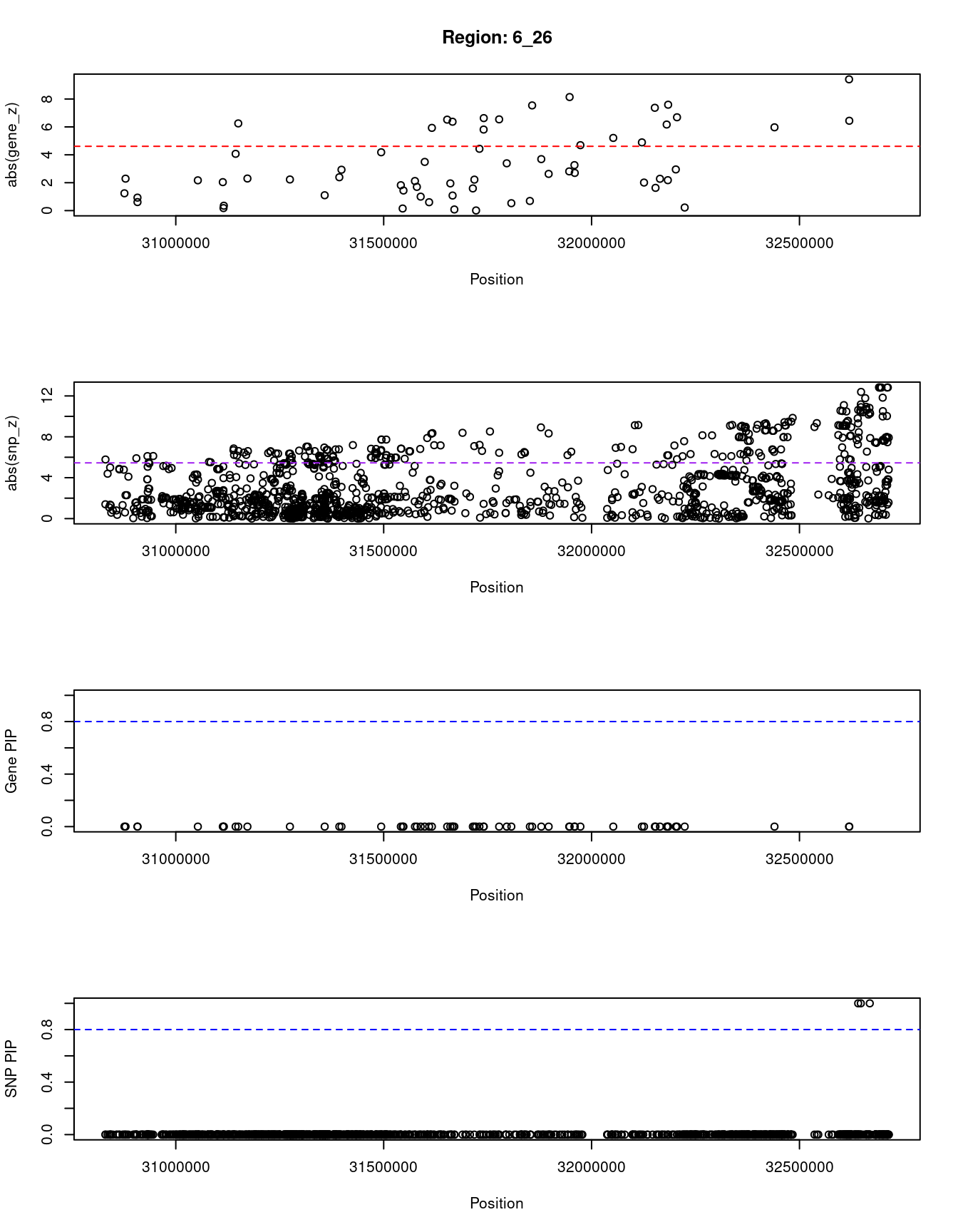

Version	Author	Date
3a7fbc1	wesleycrouse	2021-09-08

[1] "Region: 4_7"
           genename region_tag susie_pip   mu2     PVE     z
9598           EVC2        4_7     0.015  8.38 3.9e-07  1.04
892             EVC        4_7     0.072 22.37 4.8e-06  2.15
891           CRMP1        4_7     0.010  4.57 1.4e-07 -0.04
6992        JAKMIP1        4_7     0.011  5.55 1.9e-07 -0.45
2723           WFS1        4_7     0.596 63.57 1.1e-04 -8.28
241          MAN2B2        4_7     0.010  4.57 1.4e-07 -0.04
10253        MRFAP1        4_7     0.020 10.46 6.1e-07 -1.24
9279     AC093323.3        4_7     0.020 10.71 6.5e-07 -1.17
13412 RP11-539L10.3        4_7     0.011  4.87 1.5e-07 -0.25
13269 RP11-539L10.2        4_7     0.010  4.60 1.4e-07 -0.10
8116          S100P        4_7     0.011  4.96 1.6e-07 -0.37
10250      MRFAP1L1        4_7     0.119 27.27 9.6e-06  2.61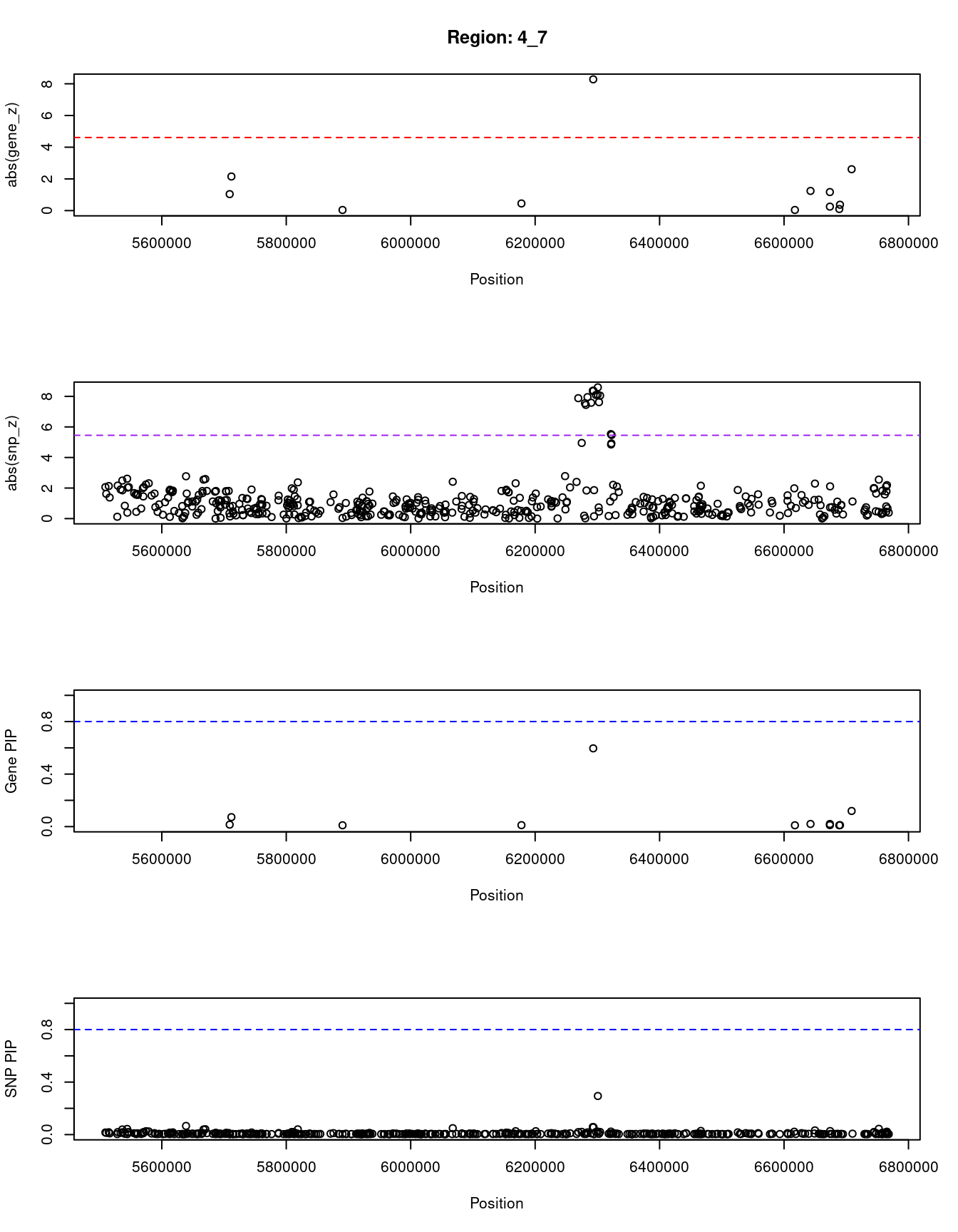

Version	Author	Date
3a7fbc1	wesleycrouse	2021-09-08

[1] "Region: 7_23"
           genename region_tag susie_pip   mu2     PVE     z
14139 CTD-2227E11.1       7_23     0.008  6.17 1.4e-07  0.57
496          NFE2L3       7_23     0.006  4.57 8.6e-08  0.05
1262          SNX10       7_23     0.056 24.27 4.0e-06  2.50
3929           CBX3       7_23     0.056 24.27 4.0e-06  2.50
3926       KIAA0087       7_23     0.047 22.63 3.2e-06  2.26
12460    AC004540.5       7_23     0.047 22.63 3.2e-06  2.26
12902    AC004947.2       7_23     0.009  8.64 2.4e-07  1.34
2392          HOXA2       7_23     0.009  7.55 2.0e-07 -0.70
11693         HOXA4       7_23     0.006  4.58 8.7e-08  0.05
2395          HOXA5       7_23     0.007  5.68 1.2e-07 -0.32
2396          HOXA6       7_23     0.008  6.16 1.4e-07 -0.46
3933          HOXA7       7_23     0.007  5.00 1.0e-07 -0.16
1058          HOXA9       7_23     0.008  6.40 1.5e-07  0.54
55           HOXA11       7_23     0.016 12.99 6.3e-07 -1.40
2402         HIBADH       7_23     0.007  5.28 1.1e-07  0.19
2403        TAX1BP1       7_23     0.007  5.90 1.3e-07  1.02
7048          JAZF1       7_23     0.728 53.35 1.2e-04  7.66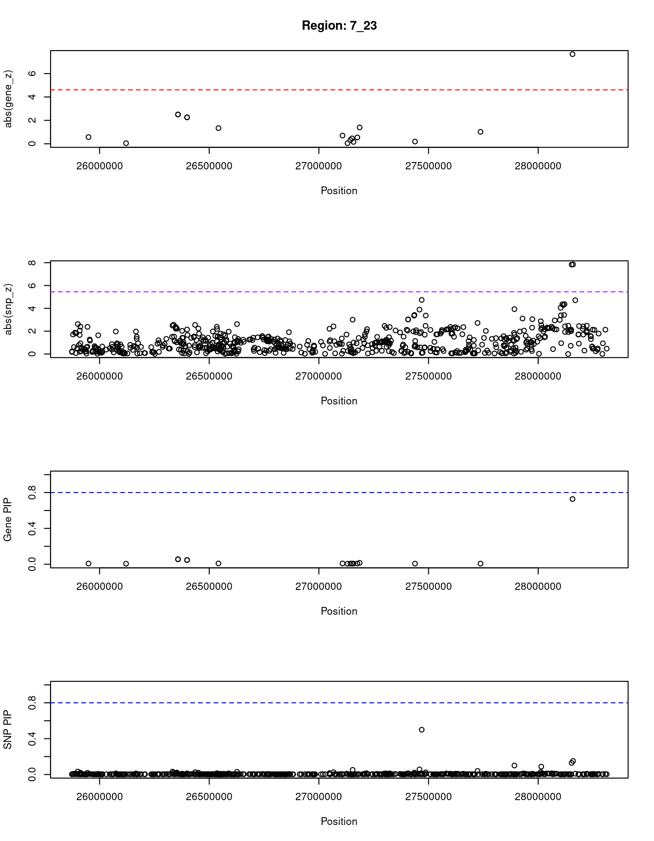

Version	Author	Date
3a7fbc1	wesleycrouse	2021-09-08

[1] "Region: 8_36"
           genename region_tag susie_pip   mu2     PVE     z
8340          ZMAT4       8_36     0.020 10.82 6.4e-07  1.17
2134          SFRP1       8_36     0.011  5.66 1.9e-07 -0.39
6549         GOLGA7       8_36     0.116 28.08 9.7e-06  3.05
6551          GINS4       8_36     0.020 19.91 1.2e-06 -3.73
7444          GPAT4       8_36     0.010  8.95 2.6e-07 -2.18
356            ANK1       8_36     0.829 40.62 1.0e-04 -6.50
13780 RP11-930P14.2       8_36     0.051 20.36 3.1e-06 -2.47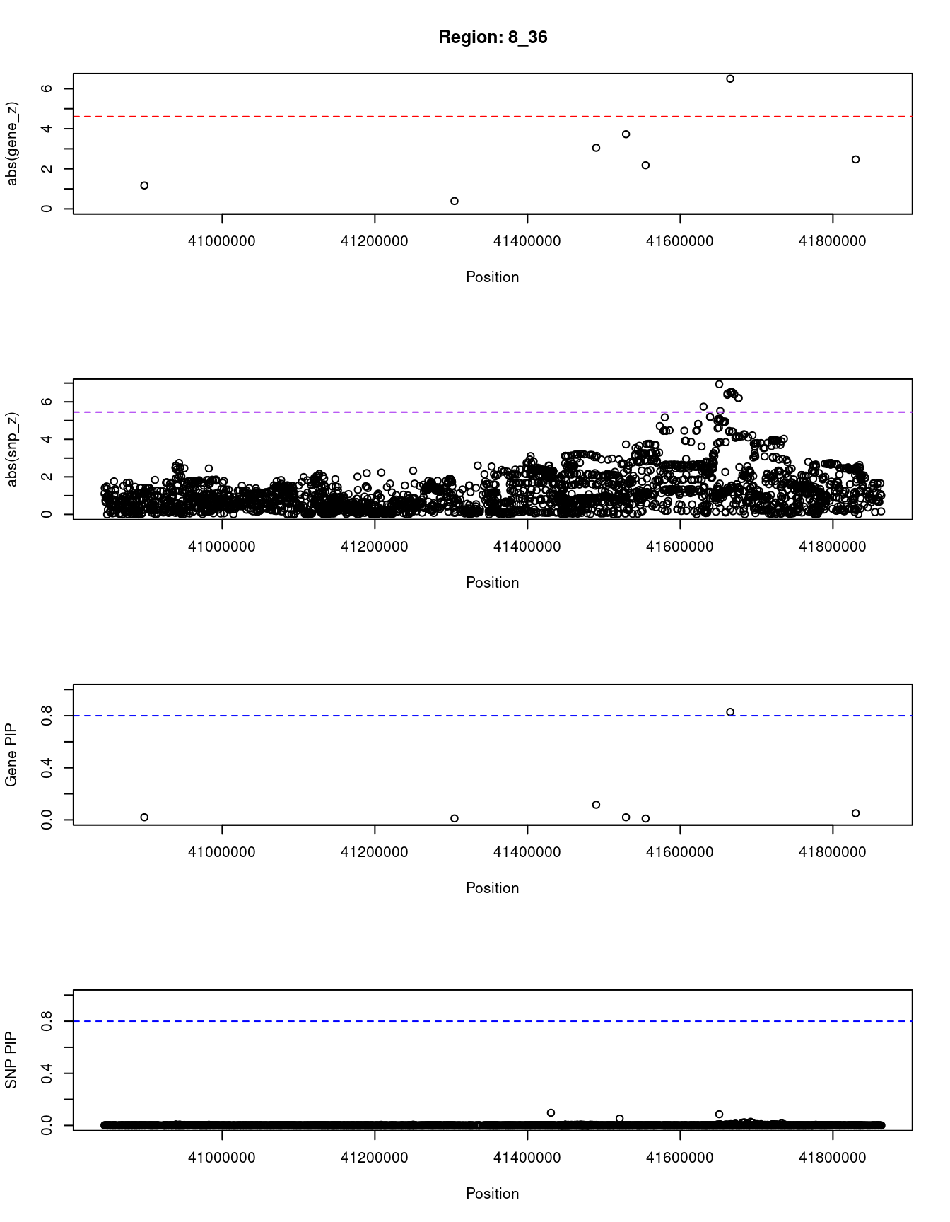

Version	Author	Date
3a7fbc1	wesleycrouse	2021-09-08

SNPs with highest PIPs

#snps with PIP>0.8 or 20 highest PIPs
head(ctwas_snp_res[order(-ctwas_snp_res$susie_pip),report_cols_snps],
max(sum(ctwas_snp_res$susie_pip>0.8), 20))

                id region_tag susie_pip     mu2     PVE     z
5205    rs56219074       1_13     1.000   64.12 1.9e-04  2.18
37018   rs75222047       1_85     1.000  812.47 2.4e-03  2.91
42580    rs2776714       1_97     1.000  804.92 2.4e-03 -2.78
65949     rs780093       2_16     1.000   42.62 1.3e-04  6.98
82161   rs12471681       2_53     1.000  928.47 2.8e-03 -3.05
140234  rs13062973       3_45     1.000  616.64 1.8e-03 -3.60
168235   rs1388475      3_107     1.000  516.37 1.5e-03  2.87
168236  rs13071192      3_107     1.000  493.46 1.5e-03 -3.12
170701  rs28661518      3_112     1.000  984.19 2.9e-03 -3.09
210519   rs2125449       4_79     1.000 1030.47 3.1e-03 -3.33
253640   rs3910018       5_51     1.000  840.58 2.5e-03 -2.86
285039   rs2206734       6_15     1.000   84.17 2.5e-04 10.34
287337  rs34662244       6_22     1.000 1754.82 5.2e-03  4.07
287355  rs67297533       6_22     1.000 1718.45 5.1e-03 -4.09
289265   rs9272679       6_26     1.000 1758.27 5.2e-03 -9.31
289274  rs17612548       6_26     1.000 1832.90 5.4e-03 11.17
289295   rs3134996       6_26     1.000 1808.42 5.4e-03 10.37
289379   rs3916765       6_27     1.000   97.94 2.9e-04 10.72
380118   rs1495743       8_20     1.000  426.67 1.3e-03  3.21
407753  rs16902104       8_83     1.000 1289.53 3.8e-03  3.51
436626   rs7025746       9_53     1.000  393.97 1.2e-03 -3.04
436630   rs2900388       9_53     1.000  386.66 1.1e-03  3.51
472037   rs2019640      10_59     1.000 1037.47 3.1e-03 -3.47
472039    rs913647      10_59     1.000 1039.87 3.1e-03  3.45
477392  rs12244851      10_70     1.000  256.46 7.6e-04 22.39
484930    rs234856       11_2     1.000   37.78 1.1e-04 -4.94
486963  rs11041828       11_6     1.000  898.91 2.7e-03  2.96
486964   rs4237770       11_6     1.000  917.68 2.7e-03 -2.93
498903 rs113527193      11_30     1.000  455.70 1.4e-03  3.29
499234  rs11603701      11_30     1.000  464.24 1.4e-03 -3.24
567100   rs9526909      13_22     1.000  735.06 2.2e-03  2.54
614351  rs12912777      15_13     1.000   33.43 9.9e-05  5.53
650842  rs12443634      16_45     1.000  194.77 5.8e-04 -3.47
650849   rs2966092      16_45     1.000  197.33 5.9e-04  3.38
656370   rs4790233       17_5     1.000  204.73 6.1e-04 -3.70
656375   rs8072531       17_5     1.000  205.45 6.1e-04 -3.98
702027  rs73537429      19_15     1.000  284.83 8.5e-04 -2.52
721423   rs2747568      20_20     1.000 1342.76 4.0e-03  3.79
721424   rs2064505      20_20     1.000 1375.04 4.1e-03 -3.92
429944   rs9410573       9_40     0.999   47.20 1.4e-04 -7.44
663260   rs9906451      17_22     0.999   30.57 9.1e-05 -5.87
702056   rs2285626      19_15     0.997  121.43 3.6e-04  5.36
380121  rs34537991       8_20     0.995  369.75 1.1e-03  3.06
574920   rs1327315      13_40     0.994   32.66 9.7e-05 -7.40
421232  rs10965243       9_16     0.992   26.51 7.8e-05 -5.41
702029  rs67238925      19_15     0.991  275.79 8.1e-04  2.39
759997   rs3129696       6_24     0.990 1625.72 4.8e-03 -3.92
436629   rs7868850       9_53     0.987   75.39 2.2e-04  0.83
316978 rs138764591       6_89     0.982   24.34 7.1e-05  2.59
168238  rs13081434      3_107     0.980  473.40 1.4e-03 -2.47
289480   rs2857161       6_27     0.977   87.70 2.5e-04  6.21
436627   rs4742930       9_53     0.973  304.65 8.8e-04  3.25
47621   rs79687284      1_109     0.960   26.04 7.4e-05  5.66
484929    rs234852       11_2     0.954   26.07 7.4e-05  3.12
29222    rs6679677       1_70     0.949   26.06 7.3e-05  5.33
407752  rs16902103       8_83     0.942 1262.88 3.5e-03 -3.50
538201    rs189339      12_40     0.942   33.37 9.3e-05 -6.27
154541  rs72964564       3_76     0.932   33.29 9.2e-05 -6.10
472117   rs1977833      10_59     0.927  101.36 2.8e-04 -8.47
256835  rs10479168       5_59     0.918   26.05 7.1e-05  5.36
170702  rs73190822      3_112     0.917  962.93 2.6e-03  3.11
574932    rs502027      13_40     0.909   31.65 8.5e-05  7.22
171586   rs6444187      3_114     0.906   25.70 6.9e-05  5.17
205072  rs35518360       4_67     0.878   24.26 6.3e-05  4.70
648085  rs72802395      16_40     0.877   35.62 9.3e-05 -6.35
535250   rs2682323      12_33     0.873   24.09 6.2e-05  4.74
778230   rs3217792       12_4     0.848   37.47 9.4e-05 -6.10
37037    rs2179109       1_85     0.843  796.04 2.0e-03 -3.03
140222  rs34695932       3_45     0.826  644.14 1.6e-03  4.13
656366  rs79425343       17_5     0.826   25.04 6.1e-05  1.15
170700  rs62287225      3_112     0.820  962.71 2.3e-03  3.08
160081  rs73148854       3_89     0.809   23.36 5.6e-05 -4.35
139500   rs3774723       3_43     0.807   25.03 6.0e-05 -4.84
709084  rs12609461      19_33     0.807   29.07 7.0e-05  5.53

SNPs with largest effect sizes

#plot PIP vs effect size
plot(ctwas_snp_res$susie_pip, ctwas_snp_res$mu2, xlab="PIP", ylab="mu^2", main="SNP PIPs vs Effect Size")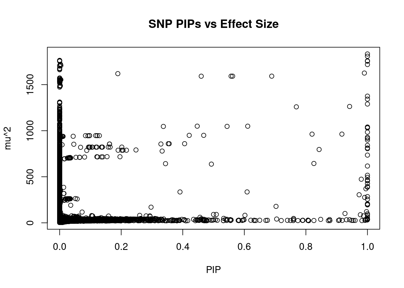

Version	Author	Date
3a7fbc1	wesleycrouse	2021-09-08

#SNPs with 50 largest effect sizes
head(ctwas_snp_res[order(-ctwas_snp_res$mu2),report_cols_snps],50)

               id region_tag susie_pip     mu2     PVE     z
289274 rs17612548       6_26     1.000 1832.90 5.4e-03 11.17
289295  rs3134996       6_26     1.000 1808.42 5.4e-03 10.37
289273 rs17612510       6_26     0.000 1763.56 1.7e-08 10.42
289281  rs9273524       6_26     0.000 1759.68 0.0e+00 10.93
289275 rs17612633       6_26     0.000 1758.58 0.0e+00 10.90
289265  rs9272679       6_26     1.000 1758.27 5.2e-03 -9.31
287337 rs34662244       6_22     1.000 1754.82 5.2e-03  4.07
289272  rs9273242       6_26     0.000 1754.81 0.0e+00 10.58
287392 rs13191786       6_22     0.003 1719.94 1.3e-05  4.10
287395 rs34218844       6_22     0.002 1719.69 1.1e-05  4.09
287355 rs67297533       6_22     1.000 1718.45 5.1e-03 -4.09
287381 rs67998226       6_22     0.004 1708.00 2.0e-05  4.25
287400 rs35030260       6_22     0.000 1706.52 1.3e-06  4.12
287386 rs33932084       6_22     0.000 1701.37 1.2e-08  3.93
287405 rs13198809       6_22     0.000 1677.89 1.3e-09  4.08
287414 rs36092177       6_22     0.000 1670.16 2.2e-10  4.08
287439 rs55690788       6_22     0.000 1661.87 1.8e-10  4.16
759997  rs3129696       6_24     0.990 1625.72 4.8e-03 -3.92
759989  rs2022083       6_24     0.189 1619.39 9.1e-04 -3.89
759944  rs2844773       6_24     0.689 1592.18 3.3e-03  3.95
759961  rs2188099       6_24     0.557 1592.09 2.6e-03  3.92
759965  rs2844770       6_24     0.562 1592.09 2.7e-03  3.92
759949  rs2844771       6_24     0.460 1591.64 2.2e-03  3.91
287551  rs1311917       6_22     0.000 1572.58 0.0e+00  3.82
287543  rs1233611       6_22     0.000 1571.53 0.0e+00  3.78
287561  rs9257192       6_22     0.000 1562.49 0.0e+00  3.92
287575  rs3135297       6_22     0.000 1561.62 0.0e+00  3.93
287580  rs9257267       6_22     0.000 1561.39 0.0e+00  3.90
760042  rs3094076       6_24     0.003 1553.73 1.6e-05  3.81
760110  rs3094629       6_24     0.004 1553.42 1.7e-05  3.81
760120  rs3129704       6_24     0.003 1552.91 1.2e-05  3.79
287597  rs3130838       6_22     0.000 1551.54 0.0e+00  3.95
760037  rs3094632       6_24     0.000 1546.87 1.4e-06  3.68
760040  rs3094077       6_24     0.000 1545.30 1.4e-06  3.69
760124  rs3129836       6_24     0.002 1545.21 1.0e-05  3.83
760121  rs3129705       6_24     0.000 1543.51 1.4e-06  3.70
760128  rs3129707       6_24     0.000 1543.22 1.0e-06  3.69
760085  rs3130398       6_24     0.000 1543.19 9.8e-07  3.68
760095  rs3130402       6_24     0.000 1543.19 9.7e-07  3.68
760097  rs9261636       6_24     0.000 1543.18 9.6e-07  3.68
760103  rs3130404       6_24     0.000 1543.17 9.5e-07  3.68
760113  rs3132656       6_24     0.000 1543.17 9.5e-07  3.68
760114  rs3132655       6_24     0.000 1543.17 9.5e-07  3.68
760049  rs3129697       6_24     0.000 1543.16 1.0e-06  3.69
760088  rs3129700       6_24     0.000 1543.16 9.4e-07  3.68
760093  rs3130401       6_24     0.000 1543.16 9.5e-07  3.68
760076  rs3129699       6_24     0.000 1543.15 9.5e-07  3.68
760115  rs3130405       6_24     0.000 1543.14 9.3e-07  3.68
760098  rs3132658       6_24     0.000 1543.13 9.2e-07  3.68
760092  rs3094073       6_24     0.000 1543.04 9.5e-07  3.68

SNPs with highest PVE

#SNPs with 50 highest pve
head(ctwas_snp_res[order(-ctwas_snp_res$PVE),report_cols_snps],50)

                id region_tag susie_pip     mu2     PVE     z
289274  rs17612548       6_26     1.000 1832.90 0.00540 11.17
289295   rs3134996       6_26     1.000 1808.42 0.00540 10.37
287337  rs34662244       6_22     1.000 1754.82 0.00520  4.07
289265   rs9272679       6_26     1.000 1758.27 0.00520 -9.31
287355  rs67297533       6_22     1.000 1718.45 0.00510 -4.09
759997   rs3129696       6_24     0.990 1625.72 0.00480 -3.92
721424   rs2064505      20_20     1.000 1375.04 0.00410 -3.92
721423   rs2747568      20_20     1.000 1342.76 0.00400  3.79
407753  rs16902104       8_83     1.000 1289.53 0.00380  3.51
407752  rs16902103       8_83     0.942 1262.88 0.00350 -3.50
759944   rs2844773       6_24     0.689 1592.18 0.00330  3.95
210519   rs2125449       4_79     1.000 1030.47 0.00310 -3.33
472037   rs2019640      10_59     1.000 1037.47 0.00310 -3.47
472039    rs913647      10_59     1.000 1039.87 0.00310  3.45
170701  rs28661518      3_112     1.000  984.19 0.00290 -3.09
407750  rs34585331       8_83     0.769 1258.92 0.00290 -3.55
82161   rs12471681       2_53     1.000  928.47 0.00280 -3.05
486963  rs11041828       11_6     1.000  898.91 0.00270  2.96
486964   rs4237770       11_6     1.000  917.68 0.00270 -2.93
759965   rs2844770       6_24     0.562 1592.09 0.00270  3.92
170702  rs73190822      3_112     0.917  962.93 0.00260  3.11
759961   rs2188099       6_24     0.557 1592.09 0.00260  3.92
253640   rs3910018       5_51     1.000  840.58 0.00250 -2.86
37018   rs75222047       1_85     1.000  812.47 0.00240  2.91
42580    rs2776714       1_97     1.000  804.92 0.00240 -2.78
170700  rs62287225      3_112     0.820  962.71 0.00230  3.08
567100   rs9526909      13_22     1.000  735.06 0.00220  2.54
759949   rs2844771       6_24     0.460 1591.64 0.00220  3.91
37037    rs2179109       1_85     0.843  796.04 0.00200 -3.03
210539  rs11721784       4_79     0.611 1048.87 0.00190  3.38
140234  rs13062973       3_45     1.000  616.64 0.00180 -3.60
210505  rs13109930       4_79     0.544 1046.98 0.00170  3.11
140222  rs34695932       3_45     0.826  644.14 0.00160  4.13
168235   rs1388475      3_107     1.000  516.37 0.00150  2.87
168236  rs13071192      3_107     1.000  493.46 0.00150 -3.12
168238  rs13081434      3_107     0.980  473.40 0.00140 -2.47
210526   rs1542437       4_79     0.447 1049.25 0.00140  3.35
498903 rs113527193      11_30     1.000  455.70 0.00140  3.29
499234  rs11603701      11_30     1.000  464.24 0.00140 -3.24
82157   rs75755471       2_53     0.468  949.72 0.00130  3.07
380118   rs1495743       8_20     1.000  426.67 0.00130  3.21
82163   rs78406274       2_53     0.421  949.54 0.00120  3.06
436626   rs7025746       9_53     1.000  393.97 0.00120 -3.04
380121  rs34537991       8_20     0.995  369.75 0.00110  3.06
436630   rs2900388       9_53     1.000  386.66 0.00110  3.51
210507   rs6819187       4_79     0.337 1046.26 0.00100  3.09
253651  rs10805847       5_51     0.406  859.00 0.00100  2.87
140228  rs13071831       3_45     0.493  637.26 0.00093  4.15
253645   rs3910025       5_51     0.356  858.84 0.00091  2.86
759989   rs2022083       6_24     0.189 1619.39 0.00091 -3.89

SNPs with largest z scores

#SNPs with 50 largest z scores
head(ctwas_snp_res[order(-abs(ctwas_snp_res$z)),report_cols_snps],50)

               id region_tag susie_pip     mu2     PVE     z
477400 rs12260037      10_70     0.003  227.92 2.3e-06 22.65
477392 rs12244851      10_70     1.000  256.46 7.6e-04 22.39
477389  rs6585198      10_70     0.001  126.84 3.1e-07 15.56
477401 rs12359102      10_70     0.000   97.20 1.3e-07 14.81
477399  rs7077039      10_70     0.000   96.94 1.3e-07 14.79
477397  rs7921525      10_70     0.000   93.63 1.4e-07 14.58
477405  rs4077527      10_70     0.000   88.00 1.3e-07 14.57
477398  rs6585203      10_70     0.000   92.71 1.4e-07 14.52
477394 rs11196191      10_70     0.000   92.53 1.4e-07 14.51
477395 rs10787472      10_70     0.001   92.11 1.4e-07 14.49
289317  rs9275221       6_26     0.000  354.03 0.0e+00 12.84
289368  rs9275583       6_26     0.000  354.14 0.0e+00 12.83
289325  rs9275275       6_26     0.000  352.61 0.0e+00 12.82
289330  rs9275307       6_26     0.000  352.88 0.0e+00 12.82
289361  rs4273728       6_26     0.000  352.97 0.0e+00 12.82
289319  rs9275223       6_26     0.000  352.43 0.0e+00 12.81
289276 rs17612712       6_26     0.000 1251.80 0.0e+00 12.39
477383 rs12243578      10_70     0.002   80.12 3.8e-07 12.36
289337  rs9275362       6_26     0.000  182.28 0.0e+00 11.83
289278  rs9273354       6_26     0.000 1185.78 0.0e+00 11.78
289274 rs17612548       6_26     1.000 1832.90 5.4e-03 11.17
289197   rs617578       6_26     0.000  259.88 0.0e+00 11.10
289281  rs9273524       6_26     0.000 1759.68 0.0e+00 10.93
289275 rs17612633       6_26     0.000 1758.58 0.0e+00 10.90
289293  rs3828800       6_26     0.000  275.02 0.0e+00 10.83
289282  rs9273528       6_26     0.000  241.46 0.0e+00 10.73
289379  rs3916765       6_27     1.000   97.94 2.9e-04 10.72
289266 rs34763586       6_26     0.000  451.05 0.0e+00 10.63
289284 rs28724252       6_26     0.000  238.50 0.0e+00 10.61
289272  rs9273242       6_26     0.000 1754.81 0.0e+00 10.58
289185  rs2760985       6_26     0.000  423.92 0.0e+00 10.56
171280 rs11929397      3_114     0.509   90.84 1.4e-04 10.55
171281 rs11716713      3_114     0.500   90.79 1.3e-04 10.55
289191  rs2647066       6_26     0.000  423.44 0.0e+00 10.52
289340  rs3135002       6_26     0.000 1051.42 0.0e+00 10.51
289210  rs3997872       6_26     0.000  424.43 0.0e+00 10.48
289273 rs17612510       6_26     0.000 1763.56 1.7e-08 10.42
289277 rs17612852       6_26     0.000 1269.51 0.0e+00 10.40
289295  rs3134996       6_26     1.000 1808.42 5.4e-03 10.37
285039  rs2206734       6_15     1.000   84.17 2.5e-04 10.34
289296  rs3134994       6_26     0.000 1165.37 0.0e+00 10.28
289290  rs3830058       6_26     0.000 1156.66 0.0e+00 10.17
289359  rs3129726       6_26     0.000 1122.49 0.0e+00 10.03
289336  rs3135190       6_26     0.000 1137.44 0.0e+00  9.99
778231 rs76895963       12_4     0.002   80.69 5.1e-07 -9.93
289170 rs12191360       6_26     0.000  454.79 0.0e+00  9.85
289263 rs41269945       6_26     0.000  444.20 0.0e+00  9.81
289221  rs3129757       6_26     0.000  766.69 0.0e+00  9.56
642712 rs79994966      16_29     0.293   75.37 6.6e-05  9.56
642708 rs17817712      16_29     0.281   75.24 6.3e-05  9.55

Gene set enrichment for genes with PIP>0.8

#GO enrichment analysis
library(enrichR)

Welcome to enrichR
Checking connection ...

Enrichr ... Connection is Live!
FlyEnrichr ... Connection is available!
WormEnrichr ... Connection is available!
YeastEnrichr ... Connection is available!
FishEnrichr ... Connection is available!

dbs <- c("GO_Biological_Process_2021", "GO_Cellular_Component_2021", "GO_Molecular_Function_2021")
genes <- ctwas_gene_res$genename[ctwas_gene_res$susie_pip>0.8]

#number of genes for gene set enrichment
length(genes)

[1] 4

if (length(genes)>0){
  GO_enrichment <- enrichr(genes, dbs)

  for (db in dbs){
    print(db)
    df <- GO_enrichment[[db]]
    df <- df[df$Adjusted.P.value<0.05,c("Term", "Overlap", "Adjusted.P.value", "Genes")]
    print(df)
  }
  
  #DisGeNET enrichment
  
  # devtools::install_bitbucket("ibi_group/disgenet2r")
  library(disgenet2r)
  
  disgenet_api_key <- get_disgenet_api_key(
                    email = "wesleycrouse@gmail.com", 
                    password = "uchicago1" )
  
  Sys.setenv(DISGENET_API_KEY= disgenet_api_key)
  
  res_enrich <-disease_enrichment(entities=genes, vocabulary = "HGNC",
                               database = "CURATED" )
  
  df <- res_enrich@qresult[1:10, c("Description", "FDR", "Ratio",  "BgRatio")]
  print(df)
  
  #WebGestalt enrichment
  library(WebGestaltR)
  
  background <- ctwas_gene_res$genename
  
  #listGeneSet()
  databases <- c("pathway_KEGG", "disease_GLAD4U", "disease_OMIM")
  
  enrichResult <- WebGestaltR(enrichMethod="ORA", organism="hsapiens",
                              interestGene=genes, referenceGene=background,
                              enrichDatabase=databases, interestGeneType="genesymbol",
                              referenceGeneType="genesymbol", isOutput=F)
  print(enrichResult[,c("description", "size", "overlap", "FDR", "database", "userId")])
}

Uploading data to Enrichr... Done.
  Querying GO_Biological_Process_2021... Done.
  Querying GO_Cellular_Component_2021... Done.
  Querying GO_Molecular_Function_2021... Done.
Parsing results... Done.
[1] "GO_Biological_Process_2021"
                                                                                                           Term
1                                                    negative regulation of gonadotropin secretion (GO:0032277)
2                                                        maintenance of apical/basal cell polarity (GO:0035090)
3                                             maintenance of epithelial cell apical/basal polarity (GO:0045199)
4                                                   positive regulation of protein phosphorylation (GO:0001934)
5                                                                     ovarian follicle development (GO:0001541)
6                                                         negative regulation of insulin secretion (GO:0046676)
7                 positive regulation of cyclin-dependent protein serine/threonine kinase activity (GO:0045737)
8                                                 negative regulation of peptide hormone secretion (GO:0090278)
9                                                               activin receptor signaling pathway (GO:0032924)
10                                 positive regulation of cyclin-dependent protein kinase activity (GO:1904031)
11                                                                        female gonad development (GO:0008585)
12                                    positive regulation of G1/S transition of mitotic cell cycle (GO:1900087)
13                           establishment or maintenance of epithelial cell apical/basal polarity (GO:0045197)
14                                                     positive regulation of reproductive process (GO:2000243)
15                                         positive regulation of cell cycle G1/S phase transition (GO:1902808)
16                                                        negative regulation of protein secretion (GO:0050709)
17                          positive regulation of pathway-restricted SMAD protein phosphorylation (GO:0010862)
18                                                negative regulation of protein metabolic process (GO:0051248)
19                                          regulation of cyclin-dependent protein kinase activity (GO:1904029)
20                                   regulation of pathway-restricted SMAD protein phosphorylation (GO:0060393)
21                                                                        fat cell differentiation (GO:0045444)
22                                      positive regulation of mitotic cell cycle phase transition (GO:1901992)
23                                                            cellular response to nutrient levels (GO:0031669)
24                                                               positive regulation of cell cycle (GO:0045787)
25                                             regulation of G1/S transition of mitotic cell cycle (GO:2000045)
26                                               negative regulation of blood vessel morphogenesis (GO:2000181)
27                         regulation of cyclin-dependent protein serine/threonine kinase activity (GO:0000079)
28                                                                             response to insulin (GO:0032868)
29                                                             negative regulation of angiogenesis (GO:0016525)
30 positive regulation of transmembrane receptor protein serine/threonine kinase signaling pathway (GO:0090100)
31                                                                 regulation of insulin secretion (GO:0050796)
32                                 positive regulation of protein serine/threonine kinase activity (GO:0071902)
33                                                   cellular response to peptide hormone stimulus (GO:0071375)
34                                          regulation of protein serine/threonine kinase activity (GO:0071900)
35                                                                       cytoskeleton organization (GO:0007010)
36                                                           cellular response to insulin stimulus (GO:0032869)
37                        transmembrane receptor protein serine/threonine kinase signaling pathway (GO:0007178)
38                                                         protein localization to plasma membrane (GO:0072659)
39                                                          protein localization to cell periphery (GO:1990778)
40                                                                 cellular response to starvation (GO:0009267)
41                                                      negative regulation of cytokine production (GO:0001818)
42                                       endoplasmic reticulum to Golgi vesicle-mediated transport (GO:0006888)
   Overlap Adjusted.P.value       Genes
1      1/5       0.02276379       INHBB
2      1/9       0.02276379        ANK1
3      1/9       0.02276379        ANK1
4    2/371       0.02276379 CCND2;INHBB
5     1/14       0.02276379       INHBB
6     1/17       0.02276379       INHBB
7     1/17       0.02276379       CCND2
8     1/18       0.02276379       INHBB
9     1/19       0.02276379       INHBB
10    1/20       0.02276379       CCND2
11    1/22       0.02276379       INHBB
12    1/26       0.02465339       CCND2
13    1/32       0.02653193        ANK1
14    1/35       0.02653193       INHBB
15    1/35       0.02653193       CCND2
16    1/39       0.02770808       INHBB
17    1/47       0.02992601       INHBB
18    1/52       0.02992601       INHBB
19    1/54       0.02992601       CCND2
20    1/58       0.02992601       INHBB
21    1/58       0.02992601       INHBB
22    1/58       0.02992601       CCND2
23    1/66       0.03119720       INHBB
24    1/66       0.03119720       CCND2
25    1/71       0.03220612       CCND2
26    1/78       0.03397975       GTF2I
27    1/82       0.03397975       CCND2
28    1/84       0.03397975       INHBB
29    1/87       0.03397975       GTF2I
30    1/92       0.03472183       INHBB
31   1/104       0.03633053       INHBB
32   1/106       0.03633053       CCND2
33   1/106       0.03633053       INHBB
34   1/111       0.03691143       CCND2
35   1/120       0.03873796        ANK1
36   1/129       0.04038846       INHBB
37   1/133       0.04038846       INHBB
38   1/136       0.04038846        ANK1
39   1/140       0.04049813        ANK1
40   1/158       0.04450223       INHBB
41   1/182       0.04952524       INHBB
42   1/185       0.04952524        ANK1
[1] "GO_Cellular_Component_2021"
                                                             Term Overlap
1                   spectrin-associated cytoskeleton (GO:0014731)     1/8
2 cyclin-dependent protein kinase holoenzyme complex (GO:0000307)    1/30
3            serine/threonine protein kinase complex (GO:1902554)    1/37
4                cytoplasmic side of plasma membrane (GO:0009898)    1/55
5       intracellular non-membrane-bounded organelle (GO:0043232)  2/1158
  Adjusted.P.value      Genes
1       0.02078867       ANK1
2       0.03197981      CCND2
3       0.03197981      CCND2
4       0.03560511       ANK1
5       0.04831435 CCND2;ANK1
[1] "GO_Molecular_Function_2021"
[1] Term             Overlap          Adjusted.P.value Genes           
<0 rows> (or 0-length row.names)
                                                          Description
38                                            Thymic epithelial tumor
50                                   SPHEROCYTOSIS, TYPE 1 (disorder)
56 MEGALENCEPHALY-POLYMICROGYRIA-POLYDACTYLY-HYDROCEPHALUS SYNDROME 3
58                                           8p11.2 deletion syndrome
17                                         Acute Myeloid Leukemia, M1
31                                            Familial Testotoxicosis
46                                      POSTAXIAL POLYDACTYLY, TYPE B
47                                    Acute Myeloid Leukemia (AML-M2)
48                                                   Alcohol Toxicity
55 MEGALENCEPHALY-POLYMICROGYRIA-POLYDACTYLY-HYDROCEPHALUS SYNDROME 1
           FDR Ratio  BgRatio
38 0.005978149   1/4   1/9703
50 0.005978149   1/4   1/9703
56 0.005978149   1/4   1/9703
58 0.005978149   1/4   1/9703
17 0.006519600   2/4 125/9703
31 0.006519600   1/4   3/9703
46 0.006519600   1/4   3/9703
47 0.006519600   2/4 125/9703
48 0.006519600   1/4   2/9703
55 0.006519600   1/4   3/9703

******************************************

*                                        *

*          Welcome to WebGestaltR !      *

*                                        *

******************************************

Loading the functional categories...
Loading the ID list...
Loading the reference list...
Performing the enrichment analysis...

Warning in oraEnrichment(interestGeneList, referenceGeneList, geneSet,
minNum = minNum, : No significant gene set is identified based on FDR 0.05!

NULL

Sensitivity, specificity and precision for silver standard genes

library("readxl")

known_annotations <- read_xlsx("data/summary_known_genes_annotations.xlsx", sheet="T2D")
known_annotations <- unique(known_annotations$`Gene Symbol`)

unrelated_genes <- ctwas_gene_res$genename[!(ctwas_gene_res$genename %in% known_annotations)]

#number of genes in known annotations
print(length(known_annotations))

[1] 72

#number of genes in known annotations with imputed expression
print(sum(known_annotations %in% ctwas_gene_res$genename))

[1] 35

#assign ctwas, TWAS, and bystander genes
ctwas_genes <- ctwas_gene_res$genename[ctwas_gene_res$susie_pip>0.8]
twas_genes <- ctwas_gene_res$genename[abs(ctwas_gene_res$z)>sig_thresh]
novel_genes <- ctwas_genes[!(ctwas_genes %in% twas_genes)]

#significance threshold for TWAS
print(sig_thresh)

[1] 4.609947

#number of ctwas genes
length(ctwas_genes)

[1] 4

#number of TWAS genes
length(twas_genes)

[1] 39

#show novel genes (ctwas genes with not in TWAS genes)
ctwas_gene_res[ctwas_gene_res$genename %in% novel_genes,report_cols]

     genename region_tag susie_pip  mu2     PVE     z
7923    INHBB       2_70     0.902 22.2 5.9e-05 -4.47

#sensitivity / recall
sensitivity <- rep(NA,2)
names(sensitivity) <- c("ctwas", "TWAS")
sensitivity["ctwas"] <- sum(ctwas_genes %in% known_annotations)/length(known_annotations)
sensitivity["TWAS"] <- sum(twas_genes %in% known_annotations)/length(known_annotations)
sensitivity

     ctwas       TWAS 
0.00000000 0.02777778

#specificity
specificity <- rep(NA,2)
names(specificity) <- c("ctwas", "TWAS")
specificity["ctwas"] <- sum(!(unrelated_genes %in% ctwas_genes))/length(unrelated_genes)
specificity["TWAS"] <- sum(!(unrelated_genes %in% twas_genes))/length(unrelated_genes)
specificity

    ctwas      TWAS 
0.9996769 0.9970111

#precision / PPV
precision <- rep(NA,2)
names(precision) <- c("ctwas", "TWAS")
precision["ctwas"] <- sum(ctwas_genes %in% known_annotations)/length(ctwas_genes)
precision["TWAS"] <- sum(twas_genes %in% known_annotations)/length(twas_genes)
precision

     ctwas       TWAS 
0.00000000 0.05128205

#ROC curves

pip_range <- (0:1000)/1000
sensitivity <- rep(NA, length(pip_range))
specificity <- rep(NA, length(pip_range))

for (index in 1:length(pip_range)){
  pip <- pip_range[index]
  ctwas_genes <- ctwas_gene_res$genename[ctwas_gene_res$susie_pip>=pip]
  sensitivity[index] <- sum(ctwas_genes %in% known_annotations)/length(known_annotations)
  specificity[index] <- sum(!(unrelated_genes %in% ctwas_genes))/length(unrelated_genes)
}

plot(1-specificity, sensitivity, type="l", xlim=c(0,1), ylim=c(0,1))

sig_thresh_range <- seq(from=0, to=max(abs(ctwas_gene_res$z)), length.out=length(pip_range))

for (index in 1:length(sig_thresh_range)){
  sig_thresh_plot <- sig_thresh_range[index]
  twas_genes <- ctwas_gene_res$genename[abs(ctwas_gene_res$z)>=sig_thresh_plot]
  sensitivity[index] <- sum(twas_genes %in% known_annotations)/length(known_annotations)
  specificity[index] <- sum(!(unrelated_genes %in% twas_genes))/length(unrelated_genes)
}

lines(1-specificity, sensitivity, xlim=c(0,1), ylim=c(0,1), col="red", lty=2)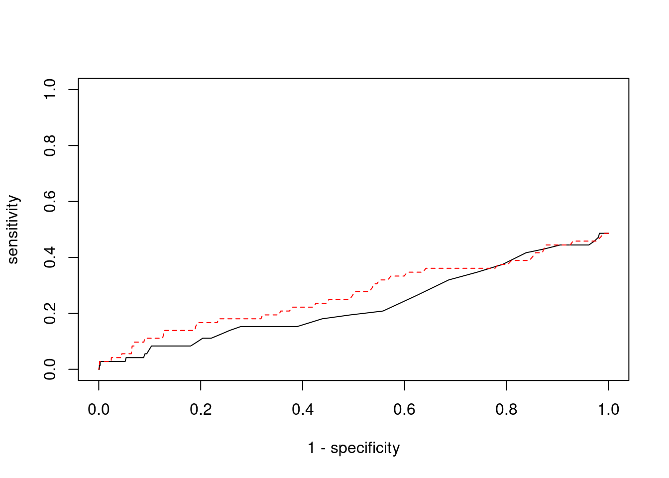

Version	Author	Date
3a7fbc1	wesleycrouse	2021-09-08

Sensitivity, specificity and precision for silver standard genes - bystanders only

This section first uses all silver standard genes to identify bystander genes within 1Mb. The silver standard and bystander gene lists are then subset to only genes with imputed expression in this analysis. Then, the ctwas and TWAS gene lists from this analysis are subset to only genes that are in the (subset) silver standard and bystander genes. These gene lists are then used to compute sensitivity, specificity and precision for ctwas and TWAS.

library(biomaRt)
library(GenomicRanges)

Loading required package: stats4

Loading required package: BiocGenerics

Loading required package: parallel


Attaching package: 'BiocGenerics'

The following objects are masked from 'package:parallel':

    clusterApply, clusterApplyLB, clusterCall, clusterEvalQ,
    clusterExport, clusterMap, parApply, parCapply, parLapply,
    parLapplyLB, parRapply, parSapply, parSapplyLB

The following objects are masked from 'package:stats':

    IQR, mad, sd, var, xtabs

The following objects are masked from 'package:base':

    anyDuplicated, append, as.data.frame, basename, cbind,
    colnames, dirname, do.call, duplicated, eval, evalq, Filter,
    Find, get, grep, grepl, intersect, is.unsorted, lapply, Map,
    mapply, match, mget, order, paste, pmax, pmax.int, pmin,
    pmin.int, Position, rank, rbind, Reduce, rownames, sapply,
    setdiff, sort, table, tapply, union, unique, unsplit, which,
    which.max, which.min

Loading required package: S4Vectors


Attaching package: 'S4Vectors'

The following object is masked from 'package:base':

    expand.grid

Loading required package: IRanges

Loading required package: GenomeInfoDb

ensembl <- useEnsembl(biomart="ENSEMBL_MART_ENSEMBL", dataset="hsapiens_gene_ensembl")
G_list <- getBM(filters= "chromosome_name", attributes= c("hgnc_symbol","chromosome_name","start_position","end_position","gene_biotype"), values=1:22, mart=ensembl)
G_list <- G_list[G_list$hgnc_symbol!="",]
G_list <- G_list[G_list$gene_biotype %in% c("protein_coding","lncRNA"),]
G_list$start <- G_list$start_position
G_list$end <- G_list$end_position
G_list_granges <- makeGRangesFromDataFrame(G_list, keep.extra.columns=T)

known_annotations_positions <- G_list[G_list$hgnc_symbol %in% known_annotations,]
half_window <- 1000000
known_annotations_positions$start <- known_annotations_positions$start_position - half_window
known_annotations_positions$end <- known_annotations_positions$end_position + half_window
known_annotations_positions$start[known_annotations_positions$start<1] <- 1
known_annotations_granges <- makeGRangesFromDataFrame(known_annotations_positions, keep.extra.columns=T)

bystanders <- findOverlaps(known_annotations_granges,G_list_granges)
bystanders <- unique(subjectHits(bystanders))
bystanders <- G_list$hgnc_symbol[bystanders]
bystanders <- bystanders[!(bystanders %in% known_annotations)]
unrelated_genes <- bystanders

#number of genes in known annotations
print(length(known_annotations))

[1] 72

#number of genes in known annotations with imputed expression
print(sum(known_annotations %in% ctwas_gene_res$genename))

[1] 35

#number of bystander genes
print(length(unrelated_genes))

[1] 1837

#number of bystander genes with imputed expression
print(sum(unrelated_genes %in% ctwas_gene_res$genename))

[1] 941

#remove genes without imputed expression from gene lists
known_annotations <- known_annotations[known_annotations %in% ctwas_gene_res$genename]
unrelated_genes <- unrelated_genes[unrelated_genes %in% ctwas_gene_res$genename]

#assign ctwas and TWAS genes
ctwas_genes <- ctwas_gene_res$genename[ctwas_gene_res$susie_pip>0.8]
twas_genes <- ctwas_gene_res$genename[abs(ctwas_gene_res$z)>sig_thresh]

#significance threshold for TWAS
print(sig_thresh)

[1] 4.609947

#number of ctwas genes
length(ctwas_genes)

[1] 4

#number of ctwas genes in known annotations or bystanders
sum(ctwas_genes %in% c(known_annotations, unrelated_genes))

[1] 0

#number of ctwas genes
length(twas_genes)

[1] 39

#number of TWAS genes
sum(twas_genes %in% c(known_annotations, unrelated_genes))

[1] 5

#remove genes not in known or bystander lists from results
ctwas_genes <- ctwas_genes[ctwas_genes %in% c(known_annotations, unrelated_genes)]
twas_genes <- twas_genes[twas_genes %in% c(known_annotations, unrelated_genes)]

#sensitivity / recall
sensitivity <- rep(NA,2)
names(sensitivity) <- c("ctwas", "TWAS")
sensitivity["ctwas"] <- sum(ctwas_genes %in% known_annotations)/length(known_annotations)
sensitivity["TWAS"] <- sum(twas_genes %in% known_annotations)/length(known_annotations)
sensitivity

     ctwas       TWAS 
0.00000000 0.05714286

#specificity
specificity <- rep(NA,2)
names(specificity) <- c("ctwas", "TWAS")
specificity["ctwas"] <- sum(!(unrelated_genes %in% ctwas_genes))/length(unrelated_genes)
specificity["TWAS"] <- sum(!(unrelated_genes %in% twas_genes))/length(unrelated_genes)
specificity

    ctwas      TWAS 
1.0000000 0.9968119

#precision / PPV
precision <- rep(NA,2)
names(precision) <- c("ctwas", "TWAS")
precision["ctwas"] <- sum(ctwas_genes %in% known_annotations)/length(ctwas_genes)
precision["TWAS"] <- sum(twas_genes %in% known_annotations)/length(twas_genes)
precision

ctwas  TWAS 
  NaN   0.4

sessionInfo()

R version 3.6.1 (2019-07-05)
Platform: x86_64-pc-linux-gnu (64-bit)
Running under: Scientific Linux 7.4 (Nitrogen)

Matrix products: default
BLAS/LAPACK: /software/openblas-0.2.19-el7-x86_64/lib/libopenblas_haswellp-r0.2.19.so

locale:
 [1] LC_CTYPE=en_US.UTF-8       LC_NUMERIC=C              
 [3] LC_TIME=en_US.UTF-8        LC_COLLATE=en_US.UTF-8    
 [5] LC_MONETARY=en_US.UTF-8    LC_MESSAGES=en_US.UTF-8   
 [7] LC_PAPER=en_US.UTF-8       LC_NAME=C                 
 [9] LC_ADDRESS=C               LC_TELEPHONE=C            
[11] LC_MEASUREMENT=en_US.UTF-8 LC_IDENTIFICATION=C       

attached base packages:
[1] parallel  stats4    stats     graphics  grDevices utils     datasets 
[8] methods   base     

other attached packages:
 [1] GenomicRanges_1.36.0 GenomeInfoDb_1.20.0  IRanges_2.18.1      
 [4] S4Vectors_0.22.1     BiocGenerics_0.30.0  biomaRt_2.40.1      
 [7] readxl_1.3.1         WebGestaltR_0.4.4    disgenet2r_0.99.2   
[10] enrichR_3.0          cowplot_1.0.0        ggplot2_3.3.3       

loaded via a namespace (and not attached):
 [1] bitops_1.0-6           fs_1.3.1               bit64_4.0.5           
 [4] doParallel_1.0.16      progress_1.2.2         httr_1.4.1            
 [7] rprojroot_2.0.2        tools_3.6.1            doRNG_1.8.2           
[10] utf8_1.2.1             R6_2.5.0               DBI_1.1.1             
[13] colorspace_1.4-1       withr_2.4.1            tidyselect_1.1.0      
[16] prettyunits_1.0.2      bit_4.0.4              curl_3.3              
[19] compiler_3.6.1         git2r_0.26.1           Biobase_2.44.0        
[22] labeling_0.3           scales_1.1.0           readr_1.4.0           
[25] stringr_1.4.0          apcluster_1.4.8        digest_0.6.20         
[28] rmarkdown_1.13         svglite_1.2.2          XVector_0.24.0        
[31] pkgconfig_2.0.3        htmltools_0.3.6        fastmap_1.1.0         
[34] rlang_0.4.11           RSQLite_2.2.7          farver_2.1.0          
[37] generics_0.0.2         jsonlite_1.6           dplyr_1.0.7           
[40] RCurl_1.98-1.1         magrittr_2.0.1         GenomeInfoDbData_1.2.1
[43] Matrix_1.2-18          Rcpp_1.0.6             munsell_0.5.0         
[46] fansi_0.5.0            gdtools_0.1.9          lifecycle_1.0.0       
[49] stringi_1.4.3          whisker_0.3-2          yaml_2.2.0            
[52] zlibbioc_1.30.0        plyr_1.8.4             grid_3.6.1            
[55] blob_1.2.1             promises_1.0.1         crayon_1.4.1          
[58] lattice_0.20-38        hms_1.1.0              knitr_1.23            
[61] pillar_1.6.1           igraph_1.2.4.1         rjson_0.2.20          
[64] rngtools_1.5           reshape2_1.4.3         codetools_0.2-16      
[67] XML_3.98-1.20          glue_1.4.2             evaluate_0.14         
[70] data.table_1.14.0      vctrs_0.3.8            httpuv_1.5.1          
[73] foreach_1.5.1          cellranger_1.1.0       gtable_0.3.0          
[76] purrr_0.3.4            assertthat_0.2.1       cachem_1.0.5          
[79] xfun_0.8               later_0.8.0            tibble_3.1.2          
[82] iterators_1.0.13       AnnotationDbi_1.46.0   memoise_2.0.0         
[85] workflowr_1.6.2        ellipsis_0.3.2

Diabetes diagnosed by doctor - Adipose_Subcutaneous

wesleycrouse

2021-09-7