Investigating MR Locus Simulation Results

workflowr

• Summary
• Checks
• Past versions

Last updated: 2023-06-12

Checks: 6 1

Knit directory: ctwas_applied/

This reproducible R Markdown analysis was created with workflowr (version 1.7.0). The Checks tab describes the reproducibility checks that were applied when the results were created. The Past versions tab lists the development history.

---

R Markdown file: uncommitted changes

The R Markdown file has unstaged changes. To know which version of the R Markdown file created these results, you’ll want to first commit it to the Git repo. If you’re still working on the analysis, you can ignore this warning. When you’re finished, you can run wflow_publish to commit the R Markdown file and build the HTML.

Environment: empty

Great job! The global environment was empty. Objects defined in the global environment can affect the analysis in your R Markdown file in unknown ways. For reproduciblity it’s best to always run the code in an empty environment.

Seed: set.seed(20210726)

The command set.seed(20210726) was run prior to running the code in the R Markdown file. Setting a seed ensures that any results that rely on randomness, e.g. subsampling or permutations, are reproducible.

Session information: recorded

Great job! Recording the operating system, R version, and package versions is critical for reproducibility.

Cache: none

Nice! There were no cached chunks for this analysis, so you can be confident that you successfully produced the results during this run.

File paths: relative

Great job! Using relative paths to the files within your workflowr project makes it easier to run your code on other machines.

Repository version: d17186e

Great! You are using Git for version control. Tracking code development and connecting the code version to the results is critical for reproducibility.

The results in this page were generated with repository version d17186e. See the Past versions tab to see a history of the changes made to the R Markdown and HTML files.

Note that you need to be careful to ensure that all relevant files for the analysis have been committed to Git prior to generating the results (you can use wflow_publish or wflow_git_commit). workflowr only checks the R Markdown file, but you know if there are other scripts or data files that it depends on. Below is the status of the Git repository when the results were generated:

Untracked files:
    Untracked:  gwas.RData
    Untracked:  ld_R_info.RData
    Untracked:  z_snp_pos_ebi-a-GCST004131.RData
    Untracked:  z_snp_pos_ebi-a-GCST004132.RData
    Untracked:  z_snp_pos_ebi-a-GCST004133.RData
    Untracked:  z_snp_pos_scz-2018.RData
    Untracked:  z_snp_pos_ukb-a-360.RData
    Untracked:  z_snp_pos_ukb-d-30780_irnt.RData

Unstaged changes:
    Modified:   analysis/simulation_MRLocus.Rmd

Note that any generated files, e.g. HTML, png, CSS, etc., are not included in this status report because it is ok for generated content to have uncommitted changes.

---

These are the previous versions of the repository in which changes were made to the R Markdown (analysis/simulation_MRLocus.Rmd) and HTML (docs/simulation_MRLocus.html) files. If you’ve configured a remote Git repository (see ?wflow_git_remote), click on the hyperlinks in the table below to view the files as they were in that past version.

File	Version	Author	Date	Message
Rmd	d17186e	wesleycrouse	2023-06-08	updating MRLocus investigation
html	d17186e	wesleycrouse	2023-06-08	updating MRLocus investigation
Rmd	7f6fbc8	wesleycrouse	2023-05-15	fixing issue with plots
html	7f6fbc8	wesleycrouse	2023-05-15	fixing issue with plots
Rmd	3e493c9	wesleycrouse	2023-05-15	adding detailed MRLocus results
html	3e493c9	wesleycrouse	2023-05-15	adding detailed MRLocus results
Rmd	dba8c0e	wesleycrouse	2023-05-14	updating simulation plot with MRLocus
Rmd	c538341	wesleycrouse	2023-04-26	fixing issue with ncausal plot

---

MRLocus in High PVE Scenario

library(data.table)
library(mrlocus)
library(ctwas)

#load weight names
weightf <- "/project2/mstephens/causalTWAS/fusion_weights/Adipose_Subcutaneous.pos"
weights <- as.data.frame(fread(weightf, header = T))
weights$ENSEMBL_ID <- sapply(weights$WGT, function(x){unlist(strsplit(unlist(strsplit(x,"/"))[2], "[.]"))[2]})

####################

results_df <- data.frame()

simutag_list <- c("4-1", "4-2", "4-3", "4-4", "4-5")
#simutag_list <- c("10-1", "10-2", "10-3", "10-4", "10-5")

####################

results_dir <- "/project2/mstephens/causalTWAS/simulations/simulation_ctwas_rss_20210416_compare/"

alpha <- 0.05

for (simutag in simutag_list){
  load(paste0("/home/wcrouse/causalTWAS/simulations/simulation_ctwas_rss_20210416/ukb-s80.45-adi_simu", simutag, "-pheno.Rd"))
  
  true_genes <- unlist(sapply(1:22, function(x){phenores$batch[[x]]$id.cgene}))
  true_genes <- weights$ENSEMBL_ID[match(true_genes, weights$ID)]
  
  n_causal <- length(true_genes)
  
  ##########

  results_files <- list.files(results_dir)
  results_files <- results_files[grep(".mrlocus.", results_files)]
  results_files <- results_files[grep(simutag, results_files)]
  
  results_files <- results_files[grep("result.batch", results_files)]
  #results_files <- results_files[grep("result.noprune", results_files)]
  results_files <- results_files[grep("_temp", results_files)]
  
  results_files <- paste0(results_dir, results_files)
  
  mrlocus_results <- lapply(results_files, function(x){as.data.frame(fread(x, header=T))})
  mrlocus_results <- do.call(rbind, mrlocus_results)
  
  ##########
  
  mrlocus_results$TP <- mrlocus_results$gene_id %in% true_genes
  
  n_genes <- nrow(mrlocus_results)
  
  n_zero_clumps <- sum(mrlocus_results$n_clumps==0)
  n_one_clump <- sum(mrlocus_results$n_clumps==1)
  
  n_sig <- sum(sign(mrlocus_results$CI_10)==sign(mrlocus_results$CI_90), na.rm=T)
  n_sig_twoplus <- sum(sign(mrlocus_results$CI_10)==sign(mrlocus_results$CI_90) & mrlocus_results$n_clumps>1, na.rm=T)
  
  n_true_positive <- sum(sign(mrlocus_results$CI_10)==sign(mrlocus_results$CI_90) & mrlocus_results$TP, na.rm=T)
  
  n_causal_oneplus_clump <- sum(mrlocus_results$n_clumps>0 & mrlocus_results$TP, na.rm=T)
  n_causal_twoplus_clumps <- sum(mrlocus_results$n_clumps>1 & mrlocus_results$TP, na.rm=T)
  
  n_tp_twoplus <- sum(sign(mrlocus_results$CI_10)==sign(mrlocus_results$CI_90) & mrlocus_results$TP & mrlocus_results$n_clumps>1, na.rm=T)
  
  
  results_current <- data.frame(simutag=simutag,
                                n_causal=n_causal,
                                n_genes=n_genes,
                                n_zero_clumps=n_zero_clumps,
                                n_one_clump=n_one_clump,
                                n_sig=n_sig,
                                n_causal_oneplus_clump=n_causal_oneplus_clump,
                                n_causal_twoplus_clumps=n_causal_twoplus_clumps,
                                n_true_positive=n_true_positive,
                                n_tp_twoplus=n_tp_twoplus,
                                n_sig_twoplus=n_sig_twoplus)
  
  results_df <- rbind(results_df, results_current)
}

results_df$percent_tp <- results_df$n_true_positive/results_df$n_sig

####################
#summary of MRLocus results for each simulation
results_df

  simutag n_causal n_genes n_zero_clumps n_one_clump n_sig
1     4-1      106    8192          1662        2884   275
2     4-2      105    8192          1681        2905   288
3     4-3      136    8192          1669        2876   331
4     4-4      132    8192          1673        2893   308
5     4-5      123    8192          1738        2860   335
  n_causal_oneplus_clump n_causal_twoplus_clumps n_true_positive n_tp_twoplus
1                     81                      49              28           13
2                     89                      53              24           10
3                     98                      47              37           16
4                    105                      51              31           12
5                    100                      55              42           19
  n_sig_twoplus percent_tp
1           118 0.10181818
2           108 0.08333333
3           133 0.11178248
4           136 0.10064935
5           131 0.12537313

#averaging over simulations
colMeans(results_df[,colnames(results_df)[2:10]])

               n_causal                 n_genes           n_zero_clumps 
                  120.4                  8192.0                  1684.6 
            n_one_clump                   n_sig  n_causal_oneplus_clump 
                 2883.6                   307.4                    94.6 
n_causal_twoplus_clumps         n_true_positive            n_tp_twoplus 
                   51.0                    32.4                    14.0 

Investigating results for a single simulation

#load weight names
weightf <- "/project2/mstephens/causalTWAS/fusion_weights/Adipose_Subcutaneous.pos"
weights <- as.data.frame(fread(weightf, header = T))
weights$ENSEMBL_ID <- sapply(weights$WGT, function(x){unlist(strsplit(unlist(strsplit(x,"/"))[2], "[.]"))[2]})

####################

#results_dir <- "/project2/mstephens/causalTWAS/simulations/simulation_ctwas_rss_20210416_compare/"
simutag <- "4-1"

####################
#load true positive genes and SNPs from simulation

load(paste0("/home/wcrouse/causalTWAS/simulations/simulation_ctwas_rss_20210416/ukb-s80.45-adi_simu", simutag, "-pheno.Rd"))

true_genes <- unlist(sapply(1:22, function(x){phenores$batch[[x]]$id.cgene}))
true_genes <- weights$ENSEMBL_ID[match(true_genes, weights$ID)]
n_causal <- length(true_genes)
true_gene_effects <- unlist(sapply(1:22, function(x){phenores$batch[[x]]$e.beta}))
names(true_gene_effects) <- true_genes

true_snps <-  unlist(sapply(1:22, function(x){phenores$batch[[x]]$id.cSNP}))
true_snp_effects <- unlist(sapply(1:22, function(x){phenores$batch[[x]]$s.theta}))
names(true_snp_effects) <- true_snps

####################
#load MRLocus results

results_files <- list.files(results_dir)
results_files <- results_files[grep(".mrlocus.result.batch", results_files)]
results_files <- results_files[grep(simutag, results_files)]
results_files <- results_files[grep("_temp", results_files)]
results_files <- paste0(results_dir, results_files)

mrlocus_results <- lapply(results_files, function(x){as.data.frame(fread(x, header=T))})
mrlocus_results <- do.call(rbind, mrlocus_results)

#load the TWAS z scores
twas <- paste0("/project2/mstephens/causalTWAS/simulations/simulation_ctwas_rss_20210416_compare/ukb-s80.45-adi_simu", simutag, ".Adipose_Subcutaneous.coloc.result")
twas <- fread(twas, header = T)
twas$gene_id <- weights$ENSEMBL_ID[match(twas$ID, weights$ID)]
mrlocus_results$twas_p <- twas$TWAS.P[match(mrlocus_results$gene_id, twas$gene_id)]

#denote significant genes
alpha <- 0.05
sig_thresh_twas <- alpha/nrow(weights)

mrlocus_results$causal <- mrlocus_results$gene_id %in% true_genes
mrlocus_results$sig <- sign(mrlocus_results$CI_10)==sign(mrlocus_results$CI_90)

#drop results for genes that did not run in MRLocus
mrlocus_results <- mrlocus_results[!is.na(mrlocus_results$sig),]

#drop results for genes that had <2 clumps
mrlocus_results <- mrlocus_results[mrlocus_results$n_clumps>1,]

#drop results that did not run in TWAS
mrlocus_results <- mrlocus_results[!is.na(mrlocus_results$twas_p),]

####################
#add cTWAS results

ctwas <- as.data.frame(data.table::fread("/project2/mstephens/causalTWAS/simulations/simulation_ctwas_rss_20210416/ukb-s80.45-adi_simu4-1_config1.susieIrss.txt"))

ctwas <- ctwas[ctwas$type=="gene",]
ctwas$gene_id <- twas$gene_id[match(ctwas$id, twas$ID)]

mrlocus_results$ctwas_pip <- ctwas$susie_pip[match(mrlocus_results$gene_id, ctwas$gene_id)]


####################
head(mrlocus_results[order(mrlocus_results$twas_p),], 20)

     chromosome         gene_id n_clumps       alpha       CI_10        CI_90
4907          7 ENSG00000243335        2 -0.81257860 -1.73396451 -0.023893658
5401          5 ENSG00000072364        3  0.68700162  0.40504926  0.982889623
4727          7 ENSG00000237310        2 -0.22902827 -0.40057137 -0.058073354
1590          5 ENSG00000164574        3  0.02016277 -0.04403925  0.085984948
6339          7 ENSG00000272568        2 -0.29833993 -0.51897487 -0.081279172
4377          7 ENSG00000229180        2 -0.12730656 -0.46592700  0.211618536
2004          7 ENSG00000169919        2 -0.20679783 -0.52218491  0.074665067
4001          6 ENSG00000215022        2  0.10704806 -0.08477306  0.295991576
1576          6 ENSG00000164385        2  0.24743372  0.10893124  0.387811428
1583          6 ENSG00000164465        2  0.19345806  0.05752564  0.349509401
1030          1 ENSG00000153898        2  0.21065411  0.02960322  0.391463748
1675         12 ENSG00000165714        2 -0.29891763 -0.56694783 -0.037006074
2157          3 ENSG00000172215        3 -0.18929235 -0.34650084 -0.034868698
1064          7 ENSG00000154710        3 -0.05042623 -0.08437666 -0.018401842
3089          2 ENSG00000184898        2 -0.35777072 -0.77628551  0.049058198
82           13 ENSG00000134874        2 -0.42808047 -1.00227600  0.155620487
265          11 ENSG00000137700        2  0.19164374 -0.08438019  0.488912649
7808          2 ENSG00000123609        2 -0.16050952 -0.38335106  0.054014761
3167         11 ENSG00000186166        3  0.15281020 -0.11921504  0.432461292
4615          7 ENSG00000234585        3 -0.02188476 -0.04405970  0.001151294
       twas_p causal   sig   ctwas_pip
4907 9.72e-33  FALSE  TRUE 0.004551816
5401 1.07e-30   TRUE  TRUE 0.548505024
4727 6.76e-30  FALSE  TRUE 0.002209191
1590 4.09e-28  FALSE FALSE 0.021123908
6339 2.03e-26   TRUE  TRUE 0.999992919
4377 1.00e-25  FALSE FALSE 0.002905230
2004 6.32e-24  FALSE FALSE 0.001692352
4001 9.21e-23   TRUE FALSE 0.999999943
1576 6.85e-21   TRUE  TRUE 0.999994211
1583 9.67e-20  FALSE  TRUE 0.606859551
1030 7.41e-19   TRUE  TRUE 0.448164858
1675 1.64e-18   TRUE  TRUE 0.999265697
2157 1.48e-17  FALSE  TRUE 0.478867838
1064 1.08e-16  FALSE  TRUE 0.001624743
3089 9.83e-16   TRUE FALSE 0.621690999
82   1.24e-15  FALSE FALSE 0.009461171
265  9.07e-15   TRUE FALSE 0.820883824
7808 2.25e-14  FALSE FALSE 0.018403307
3167 9.47e-13  FALSE FALSE 0.017768348
4615 1.11e-11  FALSE FALSE 0.044163645

ld_R_dir = "/project2/mstephens/causalTWAS/ukbiobank/ukb_LDR_s80.45/s80.45.2_LDR"
gwas <- "/project2/mstephens/causalTWAS/simulations/simulation_ctwas_rss_20210416/ukb-s80.45-adi_simu4-1.snpgwas.txt.gz"
eqtl <- "/project2/mstephens/causalTWAS/GTEx_v7_all/Adipose_Subcutaneous.allpairs_processed.txt.gz"
weightf <- "/project2/mstephens/causalTWAS/fusion_weights/Adipose_Subcutaneous.pos"
outputdir <- "/home/wcrouse/causalTWAS/simulations/simulation_ctwas_rss_20210416_compare/"
outname <- "mrlocus_report_temp"

####################

ld_bedfs <- list.files(outputdir, pattern="*.bed")
ld_bedfs <- data.frame(chr=sapply(ld_bedfs, function(x){as.numeric(unlist(strsplit(unlist(strsplit(x, "_"))[2], "chr"))[2])}),
                       file=ld_bedfs)
rownames(ld_bedfs) <- NULL
ld_bedfs <- ld_bedfs[order(ld_bedfs$chr),]
ld_bedfs$file <- paste0(outputdir, tools::file_path_sans_ext(ld_bedfs$file))

temp_dir <- paste0(outputdir, "temp_mrlocus/")
outname_base <- rev(unlist(strsplit(outname, "/")))[1]

####################
#define function for harmonization
harmonize_sumstat_ld <- function(sumstats, ldref, effect_var="z"){
  snpnames <- intersect(sumstats$id, ldref$id)

  if (length(snpnames) != 0){
    ss.idx <- which(sumstats$id %in% snpnames)
    ld.idx <- match(sumstats$id[ss.idx], ldref$id)
    qc <- ctwas:::allele.qc(sumstats$alt[ss.idx], sumstats$ref[ss.idx],
                            ldref$alt[ld.idx], ldref$ref[ld.idx])
    ifflip <- qc[["flip"]]
    ifremove <- !qc[["keep"]]

    flip.idx <- ss.idx[ifflip]
    sumstats[flip.idx, c("alt", "ref")] <- sumstats[flip.idx, c("ref", "alt")]
    sumstats[flip.idx, effect_var] <- -sumstats[flip.idx, effect_var]

    remove.idx <- ss.idx[ifremove]
    if (length(remove.idx) != 0) {
      sumstats <- sumstats[-remove.idx,,drop = F]
    }
  }
  return(sumstats)
}

####################
#load GWAS
gwas <- as.data.frame(fread(gwas, header = T))

#format GWAS data
gwas <- gwas[,!(colnames(gwas) %in% c("t.value", "PVALUE"))]

#drop variants that are non uniquely identified by ID
gwas <- gwas[!(gwas$id %in% gwas$id[duplicated(gwas$id)]),]

####################
#load weight names
weights <- as.data.frame(fread(weightf, header = T))
weights$ENSEMBL_ID <- sapply(weights$WGT, function(x){unlist(strsplit(unlist(strsplit(x,"/"))[2], "[.]"))[2]})

####################
#load eQTL; in GTEx, the eQTL effect allele is the ALT allele
eqtl <- as.data.frame(fread(eqtl, header = T))

#trim version number from ensembl IDs
eqtl_gene_id_crosswalk <- unique(eqtl$gene_id)
eqtl_gene_id_crosswalk <- data.frame(original=eqtl_gene_id_crosswalk,
                                     trimmed=sapply(eqtl_gene_id_crosswalk, function(x){unlist(strsplit(x, "[.]"))[1]}))
eqtl$gene_id <- eqtl_gene_id_crosswalk[eqtl$gene_id, "trimmed"]
eqtl <- eqtl[, c("rs_id_dbSNP147_GRCh37p13", "gene_id", "gene_name", "ref", "alt", "slope", "slope_se", "pval_nominal")]
eqtl <- dplyr::rename(eqtl, id="rs_id_dbSNP147_GRCh37p13")

#drop genes without FUSION weights
eqtl <- eqtl[eqtl$gene_id %in% weights$ENSEMBL_ID,]

#drop entries not uniquely identified by gene_id and variant id (variant not biallelic)
eqtl_unique_id_gene <- paste0(eqtl$id, eqtl$gene_id)
eqtl <- eqtl[!(eqtl_unique_id_gene %in% eqtl_unique_id_gene[duplicated(eqtl_unique_id_gene)]),]
rm(eqtl_unique_id_gene)

####################
#LD files
ld_R_files <- paste0(ld_R_dir, "/", list.files(ld_R_dir))
ld_R_files <- ld_R_files[grep(".RDS", ld_R_files)]

ld_R_info_files <- paste0(ld_R_dir, "/", list.files(ld_R_dir))
ld_R_info_files <- ld_R_info_files[grep(".Rvar", ld_R_info_files)]

ld_R_info <- lapply(1:length(ld_R_info_files), function(x){y <- fread(ld_R_info_files[x]); y$index <- x; as.data.frame(y)})
ld_R_info <- do.call(rbind, ld_R_info)

####################
#subset to SNPs in all three datasets
snplist <- intersect(intersect(gwas$id, ld_R_info$id), eqtl$id)

gwas <- gwas[gwas$id %in% snplist,]
eqtl <- eqtl[eqtl$id %in% snplist,]
ld_R_info <- ld_R_info[ld_R_info$id %in% snplist,]

rm(snplist)

####################
#harmonize GWAS to LD reference
gwas <- harmonize_sumstat_ld(gwas, ld_R_info, effect_var="Estimate")

#harmonize eQTL to LD reference
eqtl <- harmonize_sumstat_ld(eqtl, ld_R_info, effect_var="slope")

####################
#load gene location information
# gtf <- rtracklayer::import("/project2/mstephens/causalTWAS/GTEx_v7_all/gencode.v19.genes.v7.patched_contigs.gtf")
# gtf_df <- as.data.frame(gtf)
# save(gtf_df, file="/project2/mstephens/causalTWAS/GTEx_v7_all/gencode.v19.genes.v7.patched_contigs.RData")
load("/project2/mstephens/causalTWAS/GTEx_v7_all/gencode.v19.genes.v7.patched_contigs.RData")

#keep only gene-level information
gtf_df <- gtf_df[gtf_df$type=="gene",]

#trim ensembl ID version number
gtf_df$gene_id <- sapply(gtf_df$gene_id, function(x){unlist(strsplit(x, "[.]"))[1]})

#drop genes without FUSION weights
gtf_df <- gtf_df[gtf_df$gene_id %in% weights$ENSEMBL_ID,]

####################

#subset to SNPs in all three datasets again - catch discordant variants between GWAS and eQTL after harmonization
snplist <- intersect(intersect(gwas$id, ld_R_info$id), eqtl$id)
gwas <- gwas[gwas$id %in% snplist,]
eqtl <- eqtl[eqtl$id %in% snplist,]
ld_R_info <- ld_R_info[ld_R_info$id %in% snplist,]
rm(snplist)

####################

ldref_files <- readLines("/project2/mstephens/causalTWAS/ukbiobank/ukb_pgen_s80.45/ukb-s80.45.2_pgenfs.txt")
ld_pvarfs <- sapply(ldref_files, prep_pvar, outputdir = temp_dir)

save.image("/home/wcrouse/scratch-midway2/mrlocus_image.RData")

True negatives

ENSG00000164574

load("/home/wcrouse/scratch-midway2/mrlocus_image.RData")

####################
#run MR-Locus 

gene <- "ENSG00000164574"

chr <- as.numeric(gtf_df$seqnames[gtf_df$gene_id==gene])

#prepare files for plink
plink_exclude_file <- paste0(temp_dir, "ukb_chr", chr, "_s80.45.2.exclude")

if (!file.exists(plink_exclude_file)){
  #store list of SNPs in .bed file using plink
  system_cmd <- paste0("plink --bfile ",
                       ld_bedfs$file[chr],
                       " --write-snplist --out ",
                       temp_dir, "ukb_chr", chr, "_s80.45.2")
  system(system_cmd)

  #store list of duplicate SNPs in .bed file to exclude
  system_cmd <- paste0("sort ",
                       temp_dir,
                       "ukb_chr", chr, "_s80.45.2.snplist|uniq -d > ",
                       temp_dir,
                       "ukb_chr", chr, "_s80.45.2.exclude")

  system(system_cmd)
}

#clumping using plink
eqtl_current <- eqtl[eqtl$gene_id==gene,]
eqtl_current <- dplyr::rename(eqtl_current, SNP="id", P="pval_nominal")

eqtl_current_file <- paste0(temp_dir, outname_base, ".eqtl_sumstats.", gene, ".temp")
write.table(eqtl_current, file=eqtl_current_file, sep="\t", col.names=T, row.names=F, quote=F)

eqtl_clump_file <- paste0(temp_dir, outname_base, ".eqtl_clumps.", gene, ".temp")
system_cmd <- paste0("plink --bfile ",
                     ld_bedfs$file[chr],
                     " --clump ",
                     eqtl_current_file,
                     " --clump-p1 0.001 --clump-p2 1 --clump-r2 0.1 --clump-kb 500 --out ",
                     eqtl_clump_file,
                     " --exclude ",
                     plink_exclude_file)

#system(system_cmd)
print(system_cmd)

[1] "plink --bfile /home/wcrouse/causalTWAS/simulations/simulation_ctwas_rss_20210416_compare/ukb_chr5_s80.45.2.FUSION5 --clump /home/wcrouse/causalTWAS/simulations/simulation_ctwas_rss_20210416_compare/temp_mrlocus/mrlocus_report_temp.eqtl_sumstats.ENSG00000164574.temp --clump-p1 0.001 --clump-p2 1 --clump-r2 0.1 --clump-kb 500 --out /home/wcrouse/causalTWAS/simulations/simulation_ctwas_rss_20210416_compare/temp_mrlocus/mrlocus_report_temp.eqtl_clumps.ENSG00000164574.temp --exclude /home/wcrouse/causalTWAS/simulations/simulation_ctwas_rss_20210416_compare/temp_mrlocus/ukb_chr5_s80.45.2.exclude"

eqtl_clump_file <- paste0(eqtl_clump_file, ".clumped")

clumps <- read.table(eqtl_clump_file, header=T)
clumps$SP2 <- sapply(1:nrow(clumps), function(x){paste0(clumps$SNP[x], "(1),", clumps$SP2[x])})
clumps <- lapply(clumps$SP2, function(y){unname(sapply(unlist(strsplit(y, ",")), function(x){unlist(strsplit(x, "[(]"))[1]}))})
clumps <- lapply(clumps, function(x){x[x!="NONE"]})

####################

df_locus <- data.frame(id=eqtl_current$SNP, z_eqtl=eqtl_current$slope/eqtl_current$slope_se)
df_locus <- cbind(df_locus, ld_R_info[match(df_locus$id, ld_R_info$id),c("chrom","pos")])
df_locus$z_gwas <- (gwas$Estimate/gwas$Std.Error)[match(df_locus$id, gwas$id)]
df_locus$causal <- df_locus$id %in% names(true_snp_effects) 

weightf_dir <- "/project2/mstephens/causalTWAS/fusion_weights/Adipose_Subcutaneous/"
weightf_gene <- list.files(weightf_dir)
weightf_gene <- paste0(weightf_dir, weightf_gene[grep(gene, weightf_gene)])
load(weightf_gene)

df_locus$weight <- wgt.matrix[match(df_locus$id, rownames(wgt.matrix)),"lasso"]
df_locus$weight[is.na(df_locus$weight)] <- 0

df_locus$clump <- 0

for (j in 1:length(clumps)){
  df_locus$clump[df_locus$id %in% clumps[[j]]] <- j
}

#visualize input data
colors <- c("black", rainbow(length(clumps)))

par(mfrow=c(3,1))

logging::loginfo(gene)

2023-06-12 15:22:27 INFO::ENSG00000164574

par(mar=c(2.1, 4.1, 2.1, 2.1))

plot(df_locus$pos, abs(df_locus$z_gwas), xlab="", ylab="GWAS |Z|")
abline(v=df_locus$pos[df_locus$causal], col="red")

plot(df_locus$pos, abs(df_locus$z_eqtl), xlab="", ylab="eQTL SS |Z|",
     col=colors[df_locus$clump+1])
abline(v=df_locus$pos[df_locus$causal], col="red")

plot(df_locus$pos, abs(df_locus$weight), col="purple", xlab="", ylab="eQTL Lasso |wgt|")
abline(v=df_locus$pos[df_locus$causal], col="red")

breakpoints <- ld_R_info[ld_R_info$index!=c(ld_R_info$index[-1],max(ld_R_info$index)),]
breakpoints <- breakpoints[breakpoints$chrom==chr,]
breakpoints <- breakpoints[breakpoints$pos>min(df_locus$pos) & breakpoints$pos<max(df_locus$pos),]

abline(v=breakpoints$pos)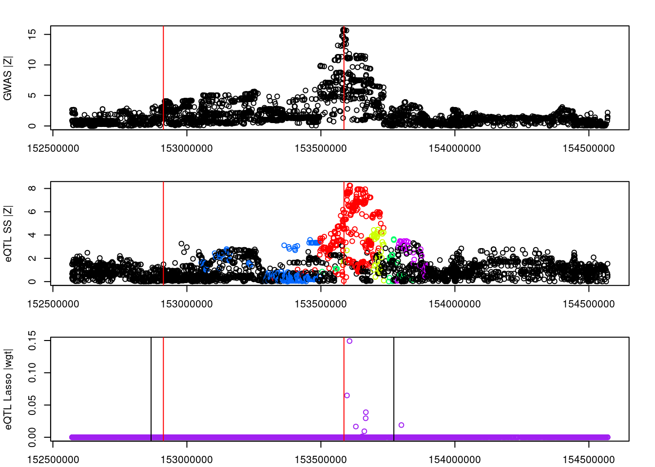

Past versions of unnamed-chunk-4-1.png

Version	Author	Date
d17186e	wesleycrouse	2023-06-08
7f6fbc8	wesleycrouse	2023-05-15
3e493c9	wesleycrouse	2023-05-15

####################

# #load LD matrix for SNPs in all clumps
# snplist_all <- unlist(clumps)
# 
# ld_R_idx <- unique(ld_R_info$index[match(snplist_all, ld_R_info$id)])
# 
# R_snp <- lapply(ld_R_files[ld_R_idx], readRDS)
# 
# R_snp_info <- lapply(ld_R_info_files[ld_R_idx], fread)
# R_snp_info <- lapply(R_snp_info, as.data.frame)
# 
# R_snp_index <- lapply(R_snp_info, function(x){x$id %in% snplist_all})
# rm(snplist_all)
# 
# for (j in 1:length(R_snp)){
#   R_snp[[j]] <- R_snp[[j]][R_snp_index[[j]],R_snp_index[[j]]]
#   R_snp_info[[j]] <- R_snp_info[[j]][R_snp_index[[j]],,drop=F]
# }
# 
# R_snp_info <- as.data.frame(do.call(rbind, R_snp_info))
# R_snp <- as.matrix(Matrix::bdiag(R_snp))
# 
# colnames(R_snp) <- R_snp_info$id
# rownames(R_snp) <- R_snp_info$id
# 
# 
# 
# R_snp_bkup <- R_snp

####################
#load genotypes and compute LD matrix for SNPs in all clumps
snplist_all <- unlist(clumps)

ld_pvarf <- ld_pvarfs[chr]
ldref_file <- ldref_files[chr]

R_snp_info <- read_pvar(ld_pvarf)
ld_pgen <- prep_pgen(pgenf = ldref_file, ld_pvarf)

sidx <- match(snplist_all, R_snp_info$id)
X.g <- read_pgen(ld_pgen, variantidx = sidx)

R_snp <- Rfast::cora(X.g)
colnames(R_snp) <- snplist_all
rownames(R_snp) <- snplist_all

rm(snplist_all, X.g)

####################

#prepare data object
data <- list(sum_stat=list(),
             ld_mat=list())

for (j in 1:length(clumps)){
  snplist <- clumps[[j]]

  R_snp_current <- R_snp[snplist,snplist,drop=F]
  dimnames(R_snp_current) <- NULL

  R_snp_info_current <- R_snp_info[match(snplist, R_snp_info$id),c("id", "ref", "alt")]

  sumstats_current <- data.frame(id=snplist,
                                 ref=R_snp_info_current$ref,
                                 eff=R_snp_info_current$alt,
                                 beta_hat_eqtl=eqtl_current$slope[match(snplist, eqtl_current$SNP)],
                                 beta_hat_gwas=gwas$Estimate[match(snplist, gwas$id)],
                                 se_eqtl=eqtl_current$slope_se[match(snplist, eqtl_current$SNP)],
                                 se_gwas=gwas$Std.Error[match(snplist, gwas$id)])
  sumstats_current$abs_z <- abs(sumstats_current$beta_hat_eqtl/sumstats_current$se_eqtl)

  data$sum_stat[[j]] <- sumstats_current
  data$ld_mat[[j]] <- R_snp_current
}

par(mfrow=c(1,1))

#collapse high correlation SNP keeping most extreme z score (most significant)
data <- collapseHighCorSNPs(data$sum_stat,
                            data$ld_mat,
                            score="abs_z",
                            plot=F)

pre:  391,53,25,236,42

post: 60,17,12,16,15

data <- flipAllelesAndGather(data$sum_stat,
                             data$ld_mat,
                             snp_id="id",
                             ref="ref",
                             a="eqtl",
                             sep="_",
                             b="gwas",
                             eff="eff",
                             beta="beta_hat",
                             se="se",
                             a2_plink="ref_eqtl",
                             alleles_same=T)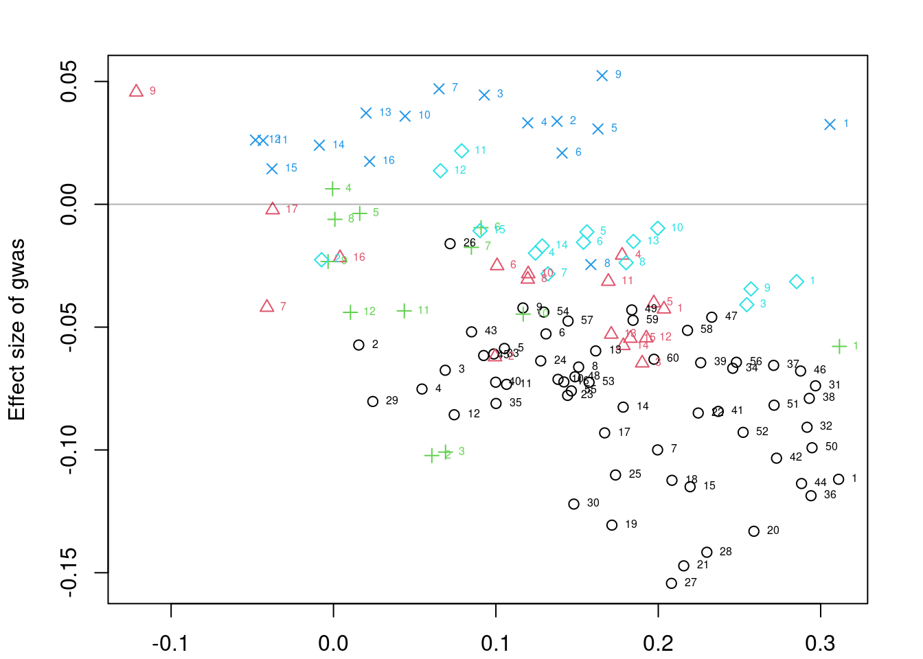

Past versions of unnamed-chunk-4-2.png

Version	Author	Date
d17186e	wesleycrouse	2023-06-08
7f6fbc8	wesleycrouse	2023-05-15
3e493c9	wesleycrouse	2023-05-15

#colocalization
coloc_fit <- list()
nclust <- length(data$beta_hat_a)

options(mc.cores=4)
for (j in 1:nclust) {
  if (length(data$beta_hat_a[[j]])>1){
    coloc_fit[[j]] <- with(data,
                           fitBetaColoc(
                             beta_hat_a = beta_hat_a[[j]],
                             beta_hat_b = beta_hat_b[[j]],
                             se_a = se_a[[j]],
                             se_b = se_b[[j]],
                             Sigma_a = Sigma[[j]],
                             Sigma_b = Sigma[[j]]
                           ))
  } else {
    coloc_fit[[j]] <- list(beta_hat_a=data$beta_hat_a[[j]],
                           beta_hat_b=data$beta_hat_b[[j]])
  }
}

Warning: There were 1837 divergent transitions after warmup. See
https://mc-stan.org/misc/warnings.html#divergent-transitions-after-warmup
to find out why this is a problem and how to eliminate them.

Warning: There were 1329 transitions after warmup that exceeded the maximum treedepth. Increase max_treedepth above 10. See
https://mc-stan.org/misc/warnings.html#maximum-treedepth-exceeded

Warning: There were 3 chains where the estimated Bayesian Fraction of Missing Information was low. See
https://mc-stan.org/misc/warnings.html#bfmi-low

Warning: Examine the pairs() plot to diagnose sampling problems

Warning: The largest R-hat is 1.68, indicating chains have not mixed.
Running the chains for more iterations may help. See
https://mc-stan.org/misc/warnings.html#r-hat

Warning: Bulk Effective Samples Size (ESS) is too low, indicating posterior means and medians may be unreliable.
Running the chains for more iterations may help. See
https://mc-stan.org/misc/warnings.html#bulk-ess

Warning: Tail Effective Samples Size (ESS) is too low, indicating posterior variances and tail quantiles may be unreliable.
Running the chains for more iterations may help. See
https://mc-stan.org/misc/warnings.html#tail-ess

Warning: There were 370 divergent transitions after warmup. See
https://mc-stan.org/misc/warnings.html#divergent-transitions-after-warmup
to find out why this is a problem and how to eliminate them.

Warning: There were 2 transitions after warmup that exceeded the maximum treedepth. Increase max_treedepth above 10. See
https://mc-stan.org/misc/warnings.html#maximum-treedepth-exceeded

Warning: Examine the pairs() plot to diagnose sampling problems

Warning: Bulk Effective Samples Size (ESS) is too low, indicating posterior means and medians may be unreliable.
Running the chains for more iterations may help. See
https://mc-stan.org/misc/warnings.html#bulk-ess

Warning: Tail Effective Samples Size (ESS) is too low, indicating posterior variances and tail quantiles may be unreliable.
Running the chains for more iterations may help. See
https://mc-stan.org/misc/warnings.html#tail-ess

Warning: There were 1106 divergent transitions after warmup. See
https://mc-stan.org/misc/warnings.html#divergent-transitions-after-warmup
to find out why this is a problem and how to eliminate them.

Warning: Examine the pairs() plot to diagnose sampling problems

Warning: The largest R-hat is 1.29, indicating chains have not mixed.
Running the chains for more iterations may help. See
https://mc-stan.org/misc/warnings.html#r-hat

Warning: Bulk Effective Samples Size (ESS) is too low, indicating posterior means and medians may be unreliable.
Running the chains for more iterations may help. See
https://mc-stan.org/misc/warnings.html#bulk-ess

Warning: Tail Effective Samples Size (ESS) is too low, indicating posterior variances and tail quantiles may be unreliable.
Running the chains for more iterations may help. See
https://mc-stan.org/misc/warnings.html#tail-ess

Warning: There were 556 divergent transitions after warmup. See
https://mc-stan.org/misc/warnings.html#divergent-transitions-after-warmup
to find out why this is a problem and how to eliminate them.

Warning: There were 999 transitions after warmup that exceeded the maximum treedepth. Increase max_treedepth above 10. See
https://mc-stan.org/misc/warnings.html#maximum-treedepth-exceeded

Warning: Examine the pairs() plot to diagnose sampling problems

Warning: The largest R-hat is 1.07, indicating chains have not mixed.
Running the chains for more iterations may help. See
https://mc-stan.org/misc/warnings.html#r-hat

Warning: Bulk Effective Samples Size (ESS) is too low, indicating posterior means and medians may be unreliable.
Running the chains for more iterations may help. See
https://mc-stan.org/misc/warnings.html#bulk-ess

Warning: Tail Effective Samples Size (ESS) is too low, indicating posterior variances and tail quantiles may be unreliable.
Running the chains for more iterations may help. See
https://mc-stan.org/misc/warnings.html#tail-ess

Warning: There were 796 divergent transitions after warmup. See
https://mc-stan.org/misc/warnings.html#divergent-transitions-after-warmup
to find out why this is a problem and how to eliminate them.

Warning: Examine the pairs() plot to diagnose sampling problems

Warning: Bulk Effective Samples Size (ESS) is too low, indicating posterior means and medians may be unreliable.
Running the chains for more iterations may help. See
https://mc-stan.org/misc/warnings.html#bulk-ess

Warning: Tail Effective Samples Size (ESS) is too low, indicating posterior variances and tail quantiles may be unreliable.
Running the chains for more iterations may help. See
https://mc-stan.org/misc/warnings.html#tail-ess

res <- list(beta_hat_a = lapply(coloc_fit, `[[`, "beta_hat_a"),
            beta_hat_b = lapply(coloc_fit, `[[`, "beta_hat_b"),
            sd_a = data$se_a,
            sd_b = data$se_b,
            alleles = data$alleles)

res <- extractForSlope(res)

Past versions of unnamed-chunk-4-3.png

Version	Author	Date
d17186e	wesleycrouse	2023-06-08
7f6fbc8	wesleycrouse	2023-05-15
3e493c9	wesleycrouse	2023-05-15

res

$beta_hat_a
[1] 0.17282472 0.09660027 0.07579629 0.26026197 0.08630545

$beta_hat_b
[1] -0.015097863 -0.029275199  0.001431053  0.019172375 -0.008445798

$sd_a
[1] 0.0376575 0.0708576 0.0853399 0.0853019 0.0818514

$sd_b
[1] 0.009967241 0.015663260 0.021558256 0.021714154 0.018479744

$alleles
             id ref eff
44   rs17553077   C   T
63    rs7737824   A   G
78   rs11746823   G   T
90     rs816007   G   A
106 rs113811083   C   T

#sort clusters by significance
res$abs_z <- abs(res$beta_hat_a/res$sd_a)
res_sig_order <- order(-res$abs_z)

res$beta_hat_a <- res$beta_hat_a[res_sig_order]
res$beta_hat_b <- res$beta_hat_b[res_sig_order]
res$sd_a <- res$sd_a[res_sig_order]
res$sd_b <- res$sd_b[res_sig_order]
res$alleles <- res$alleles[res_sig_order,,drop=F]
res$abs_z <- NULL

####################

res_bkup <- res

####################

#trim clusters if (absolute) correlation greater than 0.05
if (length(res$alleles$id)>1){
  trim_index <- trimClusters(r2=abs(R_snp[res$alleles$id,res$alleles$id,drop=F]),
                             r2_threshold=0.05)

  if (length(trim_index)>0){
    res$beta_hat_a <- res$beta_hat_a[-trim_index]
    res$beta_hat_b <- res$beta_hat_b[-trim_index]
    res$sd_a <- res$sd_a[-trim_index]
    res$sd_b <- res$sd_b[-trim_index]
    res$alleles <- res$alleles[-trim_index,,drop=F]
  }
}

####################
#visual input data

par(mfrow=c(3,1))

logging::loginfo(gene)

2023-06-12 15:24:36 INFO::ENSG00000164574

par(mar=c(2.1, 4.1, 2.1, 2.1))

plot(df_locus$pos, abs(df_locus$z_gwas), xlab="", ylab="GWAS |Z|")
abline(v=df_locus$pos[df_locus$causal], col="red")

plot(df_locus$pos, abs(df_locus$z_eqtl), xlab="", ylab="eQTL SS |Z|",
     col=colors[df_locus$clump+1])
abline(v=df_locus$pos[df_locus$causal], col="red")

plot(df_locus$pos, abs(df_locus$weight), col="purple", xlab="", ylab="eQTL Lasso |wgt|")
abline(v=df_locus$pos[df_locus$causal], col="red")

breakpoints <- ld_R_info[ld_R_info$index!=c(ld_R_info$index[-1],max(ld_R_info$index)),]
breakpoints <- breakpoints[breakpoints$chrom==chr,]
breakpoints <- breakpoints[breakpoints$pos>min(df_locus$pos) & breakpoints$pos<max(df_locus$pos),]

abline(v=breakpoints$pos)

Past versions of unnamed-chunk-4-4.png

Version	Author	Date
d17186e	wesleycrouse	2023-06-08
7f6fbc8	wesleycrouse	2023-05-15
3e493c9	wesleycrouse	2023-05-15

df_locus$trim <- F
df_locus$trim[match(res_bkup$alleles$id[trim_index], df_locus$id)] <- T
df_locus$color <- colors[df_locus$clump+1]
df_locus[match(res_bkup$alleles$id, df_locus$id),]

                 id    z_eqtl chrom       pos     z_gwas causal weight clump
4549809  rs17553077  7.653907     5 153665854 -11.405619  FALSE      0     1
4549223    rs816007  3.584141     5 153459514   1.496219  FALSE      0     4
4549544   rs7737824  2.682846     5 153596813  -4.126465  FALSE      0     2
4550146 rs113811083 -3.484155     5 153794979   1.703955  FALSE      0     5
4550092  rs11746823  3.651199     5 153771825  -2.683634  FALSE      0     3
         trim   color
4549809 FALSE #FF0000
4549223 FALSE #0066FF
4549544  TRUE #CCFF00
4550146  TRUE #CC00FF
4550092  TRUE #00FF66

par(mfrow=c(1,1))

scales::show_col(colors[c(1, res_sig_order+1)])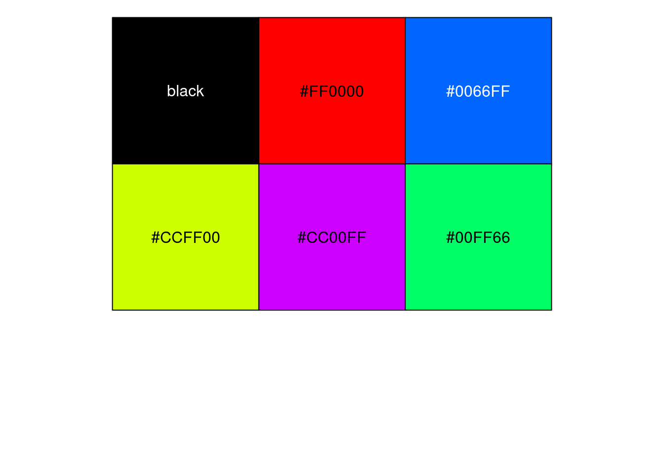

Past versions of unnamed-chunk-4-5.png

Version	Author	Date
d17186e	wesleycrouse	2023-06-08

####################

if (length(res$beta_hat_a)==1){
  #parametric sample from MRLocus code
  m <- 1e+05
  post_samples <- list(alpha=rnorm(m, res$beta_hat_b, res$sd_b)/rnorm(m, res$beta_hat_a, res$sd_a))
} else {
  #fit MRLocus slope model
  res <- fitSlope(res, iter=10000)
  post_samples <- rstan::extract(res$stanfit)
}

Warning: There were 1146 divergent transitions after warmup. See
https://mc-stan.org/misc/warnings.html#divergent-transitions-after-warmup
to find out why this is a problem and how to eliminate them.

Warning: Examine the pairs() plot to diagnose sampling problems

par(mfrow=c(1,1))

#display results
print(res$stanfit, pars=c("alpha","sigma"), probs=c(.1,.9), digits=3)

Inference for Stan model: slope.
4 chains, each with iter=10000; warmup=5000; thin=1; 
post-warmup draws per chain=5000, total post-warmup draws=20000.

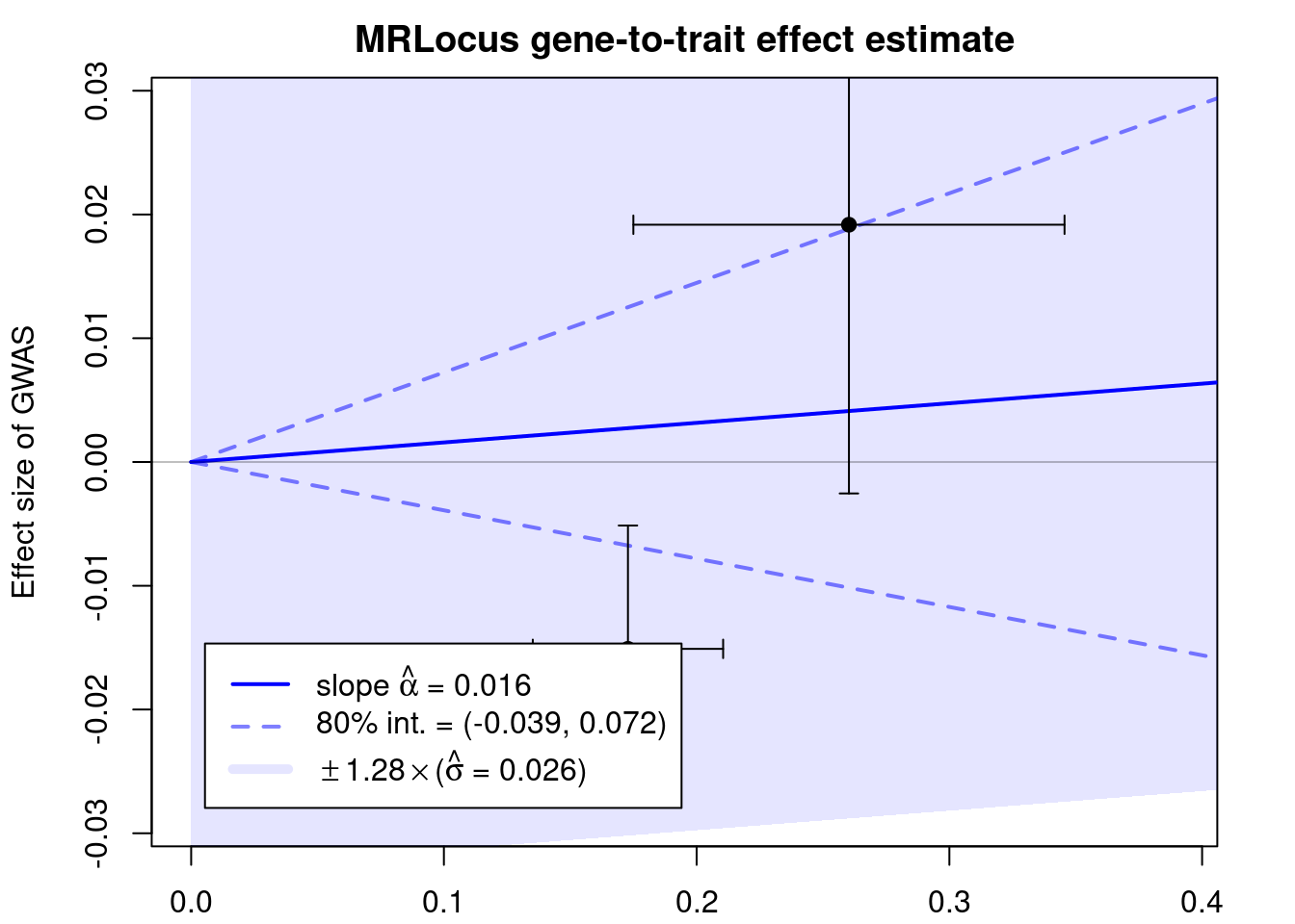
       mean se_mean    sd    10%   90% n_eff  Rhat
alpha 0.016       0 0.043 -0.039 0.072  7699 1.000
sigma 0.026       0 0.019  0.006 0.052  6145 1.001

Samples were drawn using NUTS(diag_e) at Mon Jun 12 15:24:38 2023.
For each parameter, n_eff is a crude measure of effective sample size,
and Rhat is the potential scale reduction factor on split chains (at 
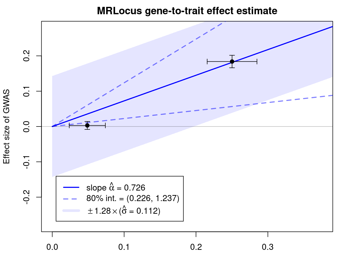
convergence, Rhat=1).

if (!is.null(res$stanfit)){
  plotMrlocus(res, main="MRLocus gene-to-trait effect estimate")
} else {
  logging::loginfo("<2 clumps for analysis")
}

Past versions of unnamed-chunk-4-6.png

Version	Author	Date
d17186e	wesleycrouse	2023-06-08

True positives

ENSG00000072364

load("/home/wcrouse/scratch-midway2/mrlocus_image.RData")

####################
#run MR-Locus 

gene <- "ENSG00000072364"

chr <- as.numeric(gtf_df$seqnames[gtf_df$gene_id==gene])

#prepare files for plink
plink_exclude_file <- paste0(temp_dir, "ukb_chr", chr, "_s80.45.2.exclude")

if (!file.exists(plink_exclude_file)){
  #store list of SNPs in .bed file using plink
  system_cmd <- paste0("plink --bfile ",
                       ld_bedfs$file[chr],
                       " --write-snplist --out ",
                       temp_dir, "ukb_chr", chr, "_s80.45.2")
  system(system_cmd)

  #store list of duplicate SNPs in .bed file to exclude
  system_cmd <- paste0("sort ",
                       temp_dir,
                       "ukb_chr", chr, "_s80.45.2.snplist|uniq -d > ",
                       temp_dir,
                       "ukb_chr", chr, "_s80.45.2.exclude")

  system(system_cmd)
}

#clumping using plink
eqtl_current <- eqtl[eqtl$gene_id==gene,]
eqtl_current <- dplyr::rename(eqtl_current, SNP="id", P="pval_nominal")

eqtl_current_file <- paste0(temp_dir, outname_base, ".eqtl_sumstats.", gene, ".temp")
write.table(eqtl_current, file=eqtl_current_file, sep="\t", col.names=T, row.names=F, quote=F)

eqtl_clump_file <- paste0(temp_dir, outname_base, ".eqtl_clumps.", gene, ".temp")
system_cmd <- paste0("plink --bfile ",
                     ld_bedfs$file[chr],
                     " --clump ",
                     eqtl_current_file,
                     " --clump-p1 0.001 --clump-p2 1 --clump-r2 0.1 --clump-kb 500 --out ",
                     eqtl_clump_file,
                     " --exclude ",
                     plink_exclude_file)

#system(system_cmd)
print(system_cmd)

[1] "plink --bfile /home/wcrouse/causalTWAS/simulations/simulation_ctwas_rss_20210416_compare/ukb_chr5_s80.45.2.FUSION5 --clump /home/wcrouse/causalTWAS/simulations/simulation_ctwas_rss_20210416_compare/temp_mrlocus/mrlocus_report_temp.eqtl_sumstats.ENSG00000072364.temp --clump-p1 0.001 --clump-p2 1 --clump-r2 0.1 --clump-kb 500 --out /home/wcrouse/causalTWAS/simulations/simulation_ctwas_rss_20210416_compare/temp_mrlocus/mrlocus_report_temp.eqtl_clumps.ENSG00000072364.temp --exclude /home/wcrouse/causalTWAS/simulations/simulation_ctwas_rss_20210416_compare/temp_mrlocus/ukb_chr5_s80.45.2.exclude"

eqtl_clump_file <- paste0(eqtl_clump_file, ".clumped")

clumps <- read.table(eqtl_clump_file, header=T)
clumps$SP2 <- sapply(1:nrow(clumps), function(x){paste0(clumps$SNP[x], "(1),", clumps$SP2[x])})
clumps <- lapply(clumps$SP2, function(y){unname(sapply(unlist(strsplit(y, ",")), function(x){unlist(strsplit(x, "[(]"))[1]}))})
clumps <- lapply(clumps, function(x){x[x!="NONE"]})

####################

df_locus <- data.frame(id=eqtl_current$SNP, z_eqtl=eqtl_current$slope/eqtl_current$slope_se)
df_locus <- cbind(df_locus, ld_R_info[match(df_locus$id, ld_R_info$id),c("chrom","pos")])
df_locus$z_gwas <- (gwas$Estimate/gwas$Std.Error)[match(df_locus$id, gwas$id)]
df_locus$causal <- df_locus$id %in% names(true_snp_effects) 

weightf_dir <- "/project2/mstephens/causalTWAS/fusion_weights/Adipose_Subcutaneous/"
weightf_gene <- list.files(weightf_dir)
weightf_gene <- paste0(weightf_dir, weightf_gene[grep(gene, weightf_gene)])
load(weightf_gene)

df_locus$weight <- wgt.matrix[match(df_locus$id, rownames(wgt.matrix)),"lasso"]
df_locus$weight[is.na(df_locus$weight)] <- 0

df_locus$clump <- 0

for (j in 1:length(clumps)){
  df_locus$clump[df_locus$id %in% clumps[[j]]] <- j
}

#visualize input data
colors <- c("black", rainbow(length(clumps)))

par(mfrow=c(3,1))

logging::loginfo(gene)

2023-06-12 15:25:24 INFO::ENSG00000072364

par(mar=c(2.1, 4.1, 2.1, 2.1))

plot(df_locus$pos, abs(df_locus$z_gwas), xlab="", ylab="GWAS |Z|")
abline(v=df_locus$pos[df_locus$causal], col="red")

plot(df_locus$pos, abs(df_locus$z_eqtl), xlab="", ylab="eQTL SS |Z|",
     col=colors[df_locus$clump+1])
abline(v=df_locus$pos[df_locus$causal], col="red")

plot(df_locus$pos, abs(df_locus$weight), col="purple", xlab="", ylab="eQTL Lasso |wgt|")
abline(v=df_locus$pos[df_locus$causal], col="red")

breakpoints <- ld_R_info[ld_R_info$index!=c(ld_R_info$index[-1],max(ld_R_info$index)),]
breakpoints <- breakpoints[breakpoints$chrom==chr,]
breakpoints <- breakpoints[breakpoints$pos>min(df_locus$pos) & breakpoints$pos<max(df_locus$pos),]

abline(v=breakpoints$pos)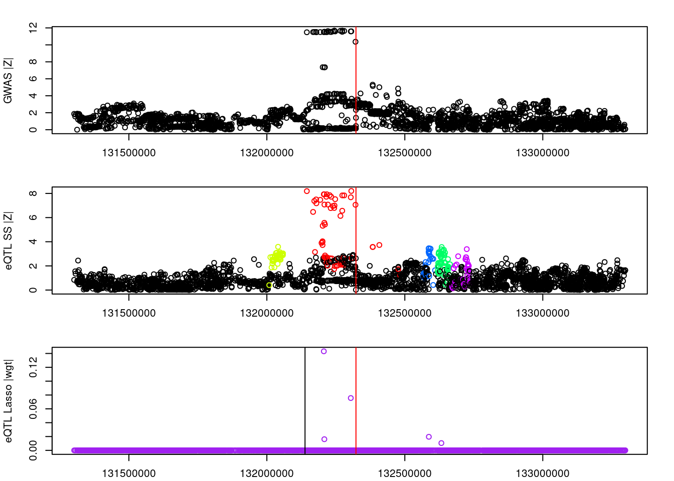

Past versions of unnamed-chunk-5-1.png

Version	Author	Date
d17186e	wesleycrouse	2023-06-08
7f6fbc8	wesleycrouse	2023-05-15
3e493c9	wesleycrouse	2023-05-15

####################

# #load LD matrix for SNPs in all clumps
# snplist_all <- unlist(clumps)
# 
# ld_R_idx <- unique(ld_R_info$index[match(snplist_all, ld_R_info$id)])
# 
# R_snp <- lapply(ld_R_files[ld_R_idx], readRDS)
# 
# R_snp_info <- lapply(ld_R_info_files[ld_R_idx], fread)
# R_snp_info <- lapply(R_snp_info, as.data.frame)
# 
# R_snp_index <- lapply(R_snp_info, function(x){x$id %in% snplist_all})
# rm(snplist_all)
# 
# for (j in 1:length(R_snp)){
#   R_snp[[j]] <- R_snp[[j]][R_snp_index[[j]],R_snp_index[[j]]]
#   R_snp_info[[j]] <- R_snp_info[[j]][R_snp_index[[j]],,drop=F]
# }
# 
# R_snp_info <- as.data.frame(do.call(rbind, R_snp_info))
# R_snp <- as.matrix(Matrix::bdiag(R_snp))
# 
# colnames(R_snp) <- R_snp_info$id
# rownames(R_snp) <- R_snp_info$id
# 
# 
# 
# R_snp_bkup <- R_snp

####################
#load genotypes and compute LD matrix for SNPs in all clumps
snplist_all <- unlist(clumps)

ld_pvarf <- ld_pvarfs[chr]
ldref_file <- ldref_files[chr]

R_snp_info <- read_pvar(ld_pvarf)
ld_pgen <- prep_pgen(pgenf = ldref_file, ld_pvarf)

sidx <- match(snplist_all, R_snp_info$id)
X.g <- read_pgen(ld_pgen, variantidx = sidx)

R_snp <- Rfast::cora(X.g)
colnames(R_snp) <- snplist_all
rownames(R_snp) <- snplist_all

rm(snplist_all, X.g)

####################

#prepare data object
data <- list(sum_stat=list(),
             ld_mat=list())

for (j in 1:length(clumps)){
  snplist <- clumps[[j]]

  R_snp_current <- R_snp[snplist,snplist,drop=F]
  dimnames(R_snp_current) <- NULL

  R_snp_info_current <- R_snp_info[match(snplist, R_snp_info$id),c("id", "ref", "alt")]

  sumstats_current <- data.frame(id=snplist,
                                 ref=R_snp_info_current$ref,
                                 eff=R_snp_info_current$alt,
                                 beta_hat_eqtl=eqtl_current$slope[match(snplist, eqtl_current$SNP)],
                                 beta_hat_gwas=gwas$Estimate[match(snplist, gwas$id)],
                                 se_eqtl=eqtl_current$slope_se[match(snplist, eqtl_current$SNP)],
                                 se_gwas=gwas$Std.Error[match(snplist, gwas$id)])
  sumstats_current$abs_z <- abs(sumstats_current$beta_hat_eqtl/sumstats_current$se_eqtl)

  data$sum_stat[[j]] <- sumstats_current
  data$ld_mat[[j]] <- R_snp_current
}

par(mfrow=c(1,1))

#collapse high correlation SNP keeping most extreme z score (most significant)
data <- collapseHighCorSNPs(data$sum_stat,
                            data$ld_mat,
                            score="abs_z",
                            plot=F)

pre:  63,44,62,27,42

post: 10,06,27,17,22

data <- flipAllelesAndGather(data$sum_stat,
                             data$ld_mat,
                             snp_id="id",
                             ref="ref",
                             a="eqtl",
                             sep="_",
                             b="gwas",
                             eff="eff",
                             beta="beta_hat",
                             se="se",
                             a2_plink="ref_eqtl",
                             alleles_same=T)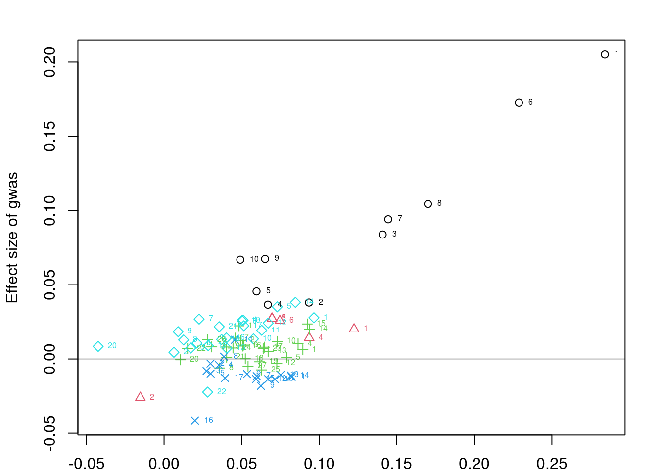

Past versions of unnamed-chunk-5-2.png

Version	Author	Date
d17186e	wesleycrouse	2023-06-08
7f6fbc8	wesleycrouse	2023-05-15
3e493c9	wesleycrouse	2023-05-15

#colocalization
coloc_fit <- list()
nclust <- length(data$beta_hat_a)

options(mc.cores=4)
for (j in 1:nclust) {
  if (length(data$beta_hat_a[[j]])>1){
    coloc_fit[[j]] <- with(data,
                           fitBetaColoc(
                             beta_hat_a = beta_hat_a[[j]],
                             beta_hat_b = beta_hat_b[[j]],
                             se_a = se_a[[j]],
                             se_b = se_b[[j]],
                             Sigma_a = Sigma[[j]],
                             Sigma_b = Sigma[[j]]
                           ))
  } else {
    coloc_fit[[j]] <- list(beta_hat_a=data$beta_hat_a[[j]],
                           beta_hat_b=data$beta_hat_b[[j]])
  }
}

Warning: There were 785 divergent transitions after warmup. See
https://mc-stan.org/misc/warnings.html#divergent-transitions-after-warmup
to find out why this is a problem and how to eliminate them.

Warning: Examine the pairs() plot to diagnose sampling problems

Warning: The largest R-hat is 1.24, indicating chains have not mixed.
Running the chains for more iterations may help. See
https://mc-stan.org/misc/warnings.html#r-hat

Warning: Bulk Effective Samples Size (ESS) is too low, indicating posterior means and medians may be unreliable.
Running the chains for more iterations may help. See
https://mc-stan.org/misc/warnings.html#bulk-ess

Warning: Tail Effective Samples Size (ESS) is too low, indicating posterior variances and tail quantiles may be unreliable.
Running the chains for more iterations may help. See
https://mc-stan.org/misc/warnings.html#tail-ess

Warning: There were 890 divergent transitions after warmup. See
https://mc-stan.org/misc/warnings.html#divergent-transitions-after-warmup
to find out why this is a problem and how to eliminate them.

Warning: Examine the pairs() plot to diagnose sampling problems

Warning: The largest R-hat is 1.32, indicating chains have not mixed.
Running the chains for more iterations may help. See
https://mc-stan.org/misc/warnings.html#r-hat

Warning: Bulk Effective Samples Size (ESS) is too low, indicating posterior means and medians may be unreliable.
Running the chains for more iterations may help. See
https://mc-stan.org/misc/warnings.html#bulk-ess

Warning: Tail Effective Samples Size (ESS) is too low, indicating posterior variances and tail quantiles may be unreliable.
Running the chains for more iterations may help. See
https://mc-stan.org/misc/warnings.html#tail-ess

Warning: There were 1652 divergent transitions after warmup. See
https://mc-stan.org/misc/warnings.html#divergent-transitions-after-warmup
to find out why this is a problem and how to eliminate them.

Warning: There were 579 transitions after warmup that exceeded the maximum treedepth. Increase max_treedepth above 10. See
https://mc-stan.org/misc/warnings.html#maximum-treedepth-exceeded

Warning: There were 3 chains where the estimated Bayesian Fraction of Missing Information was low. See
https://mc-stan.org/misc/warnings.html#bfmi-low

Warning: Examine the pairs() plot to diagnose sampling problems

Warning: The largest R-hat is 1.61, indicating chains have not mixed.
Running the chains for more iterations may help. See
https://mc-stan.org/misc/warnings.html#r-hat

Warning: Bulk Effective Samples Size (ESS) is too low, indicating posterior means and medians may be unreliable.
Running the chains for more iterations may help. See
https://mc-stan.org/misc/warnings.html#bulk-ess

Warning: Tail Effective Samples Size (ESS) is too low, indicating posterior variances and tail quantiles may be unreliable.
Running the chains for more iterations may help. See
https://mc-stan.org/misc/warnings.html#tail-ess

Warning: There were 701 divergent transitions after warmup. See
https://mc-stan.org/misc/warnings.html#divergent-transitions-after-warmup
to find out why this is a problem and how to eliminate them.

Warning: There were 45 transitions after warmup that exceeded the maximum treedepth. Increase max_treedepth above 10. See
https://mc-stan.org/misc/warnings.html#maximum-treedepth-exceeded

Warning: There were 1 chains where the estimated Bayesian Fraction of Missing Information was low. See
https://mc-stan.org/misc/warnings.html#bfmi-low

Warning: Examine the pairs() plot to diagnose sampling problems

Warning: The largest R-hat is 1.05, indicating chains have not mixed.
Running the chains for more iterations may help. See
https://mc-stan.org/misc/warnings.html#r-hat

Warning: Bulk Effective Samples Size (ESS) is too low, indicating posterior means and medians may be unreliable.
Running the chains for more iterations may help. See
https://mc-stan.org/misc/warnings.html#bulk-ess

Warning: Tail Effective Samples Size (ESS) is too low, indicating posterior variances and tail quantiles may be unreliable.
Running the chains for more iterations may help. See
https://mc-stan.org/misc/warnings.html#tail-ess

Warning: There were 856 divergent transitions after warmup. See
https://mc-stan.org/misc/warnings.html#divergent-transitions-after-warmup
to find out why this is a problem and how to eliminate them.

Warning: There were 144 transitions after warmup that exceeded the maximum treedepth. Increase max_treedepth above 10. See
https://mc-stan.org/misc/warnings.html#maximum-treedepth-exceeded

Warning: There were 3 chains where the estimated Bayesian Fraction of Missing Information was low. See
https://mc-stan.org/misc/warnings.html#bfmi-low

Warning: Examine the pairs() plot to diagnose sampling problems

Warning: The largest R-hat is 1.08, indicating chains have not mixed.
Running the chains for more iterations may help. See
https://mc-stan.org/misc/warnings.html#r-hat

Warning: Bulk Effective Samples Size (ESS) is too low, indicating posterior means and medians may be unreliable.
Running the chains for more iterations may help. See
https://mc-stan.org/misc/warnings.html#bulk-ess

Warning: Tail Effective Samples Size (ESS) is too low, indicating posterior variances and tail quantiles may be unreliable.
Running the chains for more iterations may help. See
https://mc-stan.org/misc/warnings.html#tail-ess

res <- list(beta_hat_a = lapply(coloc_fit, `[[`, "beta_hat_a"),
            beta_hat_b = lapply(coloc_fit, `[[`, "beta_hat_b"),
            sd_a = data$se_a,
            sd_b = data$se_b,
            alleles = data$alleles)

res <- extractForSlope(res)

Past versions of unnamed-chunk-5-3.png

Version	Author	Date
d17186e	wesleycrouse	2023-06-08
7f6fbc8	wesleycrouse	2023-05-15
3e493c9	wesleycrouse	2023-05-15

res

$beta_hat_a
[1] 0.25018837 0.05824561 0.04875937 0.01657236 0.02099882

$beta_hat_b
[1]  0.183939946  0.002743535  0.002980109 -0.001716928  0.011542343

$sd_a
[1] 0.0346275 0.0342004 0.0251199 0.0239703 0.0344152

$sd_b
[1] 0.01768557 0.01568073 0.01124450 0.01034667 0.01403960

$alleles
           id ref eff
1  rs11951542   A   G
11 rs10069772   G   A
17  rs6893561   C   T
57  rs1560086   G   A
74 rs11738464   C   T

#sort clusters by significance
res$abs_z <- abs(res$beta_hat_a/res$sd_a)
res_sig_order <- order(-res$abs_z)

res$beta_hat_a <- res$beta_hat_a[res_sig_order]
res$beta_hat_b <- res$beta_hat_b[res_sig_order]
res$sd_a <- res$sd_a[res_sig_order]
res$sd_b <- res$sd_b[res_sig_order]
res$alleles <- res$alleles[res_sig_order,,drop=F]
res$abs_z <- NULL

####################

res_bkup <- res

####################

#trim clusters if (absolute) correlation greater than 0.05
if (length(res$alleles$id)>1){
  trim_index <- trimClusters(r2=abs(R_snp[res$alleles$id,res$alleles$id,drop=F]),
                             r2_threshold=0.05)

  if (length(trim_index)>0){
    res$beta_hat_a <- res$beta_hat_a[-trim_index]
    res$beta_hat_b <- res$beta_hat_b[-trim_index]
    res$sd_a <- res$sd_a[-trim_index]
    res$sd_b <- res$sd_b[-trim_index]
    res$alleles <- res$alleles[-trim_index,,drop=F]
  }
}

####################
#visual input data

par(mfrow=c(3,1))

logging::loginfo(gene)

2023-06-12 15:26:33 INFO::ENSG00000072364

par(mar=c(2.1, 4.1, 2.1, 2.1))

plot(df_locus$pos, abs(df_locus$z_gwas), xlab="", ylab="GWAS |Z|")
abline(v=df_locus$pos[df_locus$causal], col="red")

plot(df_locus$pos, abs(df_locus$z_eqtl), xlab="", ylab="eQTL SS |Z|",
     col=colors[df_locus$clump+1])
abline(v=df_locus$pos[df_locus$causal], col="red")

plot(df_locus$pos, abs(df_locus$weight), col="purple", xlab="", ylab="eQTL Lasso |wgt|")
abline(v=df_locus$pos[df_locus$causal], col="red")

breakpoints <- ld_R_info[ld_R_info$index!=c(ld_R_info$index[-1],max(ld_R_info$index)),]
breakpoints <- breakpoints[breakpoints$chrom==chr,]
breakpoints <- breakpoints[breakpoints$pos>min(df_locus$pos) & breakpoints$pos<max(df_locus$pos),]

abline(v=breakpoints$pos)

Past versions of unnamed-chunk-5-4.png

Version	Author	Date
d17186e	wesleycrouse	2023-06-08
7f6fbc8	wesleycrouse	2023-05-15
3e493c9	wesleycrouse	2023-05-15

df_locus$trim <- F
df_locus$trim[match(res_bkup$alleles$id[trim_index], df_locus$id)] <- T
df_locus$color <- colors[df_locus$clump+1]
df_locus[match(res_bkup$alleles$id, df_locus$id),]

                id    z_eqtl chrom       pos      z_gwas causal weight clump
4499187 rs11951542 -8.205588     5 132306035 -11.5950440  FALSE      0     1
4499879  rs6893561  3.562638     5 132633568   0.5539217  FALSE      0     3
4498713 rs10069772  3.581654     5 132040688   1.2824300  FALSE      0     2
4499818  rs1560086  3.415952     5 132593410  -1.0714512  FALSE      0     4
4500078 rs11738464  2.460846     5 132725193   2.7154882  FALSE      0     5
         trim   color
4499187 FALSE #FF0000
4499879 FALSE #00FF66
4498713  TRUE #CCFF00
4499818  TRUE #0066FF
4500078  TRUE #CC00FF

par(mfrow=c(1,1))

scales::show_col(colors[c(1, res_sig_order+1)])

Past versions of unnamed-chunk-5-5.png

Version	Author	Date
d17186e	wesleycrouse	2023-06-08

####################

if (length(res$beta_hat_a)==1){
  #parametric sample from MRLocus code
  m <- 1e+05
  post_samples <- list(alpha=rnorm(m, res$beta_hat_b, res$sd_b)/rnorm(m, res$beta_hat_a, res$sd_a))
} else {
  #fit MRLocus slope model
  res <- fitSlope(res, iter=10000)
  post_samples <- rstan::extract(res$stanfit)
}

Warning: There were 2241 divergent transitions after warmup. See
https://mc-stan.org/misc/warnings.html#divergent-transitions-after-warmup
to find out why this is a problem and how to eliminate them.

Warning: Examine the pairs() plot to diagnose sampling problems

par(mfrow=c(1,1))

#display results
print(res$stanfit, pars=c("alpha","sigma"), probs=c(.1,.9), digits=3)

Inference for Stan model: slope.
4 chains, each with iter=10000; warmup=5000; thin=1; 
post-warmup draws per chain=5000, total post-warmup draws=20000.

       mean se_mean   sd   10%   90% n_eff Rhat
alpha 0.726   0.005 0.49 0.226 1.237  8293    1
sigma 0.112   0.002 0.10 0.022 0.246  4074    1

Samples were drawn using NUTS(diag_e) at Mon Jun 12 15:26:34 2023.
For each parameter, n_eff is a crude measure of effective sample size,
and Rhat is the potential scale reduction factor on split chains (at 
convergence, Rhat=1).

if (!is.null(res$stanfit)){
  plotMrlocus(res, main="MRLocus gene-to-trait effect estimate")
} else {
  logging::loginfo("<2 clumps for analysis")
}

Past versions of unnamed-chunk-5-6.png

Version	Author	Date
d17186e	wesleycrouse	2023-06-08

ENSG00000272568

load("/home/wcrouse/scratch-midway2/mrlocus_image.RData")

####################
#run MR-Locus 

gene <- "ENSG00000272568"

chr <- as.numeric(gtf_df$seqnames[gtf_df$gene_id==gene])

#prepare files for plink
plink_exclude_file <- paste0(temp_dir, "ukb_chr", chr, "_s80.45.2.exclude")

if (!file.exists(plink_exclude_file)){
  #store list of SNPs in .bed file using plink
  system_cmd <- paste0("plink --bfile ",
                       ld_bedfs$file[chr],
                       " --write-snplist --out ",
                       temp_dir, "ukb_chr", chr, "_s80.45.2")
  system(system_cmd)

  #store list of duplicate SNPs in .bed file to exclude
  system_cmd <- paste0("sort ",
                       temp_dir,
                       "ukb_chr", chr, "_s80.45.2.snplist|uniq -d > ",
                       temp_dir,
                       "ukb_chr", chr, "_s80.45.2.exclude")

  system(system_cmd)
}

#clumping using plink
eqtl_current <- eqtl[eqtl$gene_id==gene,]
eqtl_current <- dplyr::rename(eqtl_current, SNP="id", P="pval_nominal")

eqtl_current_file <- paste0(temp_dir, outname_base, ".eqtl_sumstats.", gene, ".temp")
write.table(eqtl_current, file=eqtl_current_file, sep="\t", col.names=T, row.names=F, quote=F)

eqtl_clump_file <- paste0(temp_dir, outname_base, ".eqtl_clumps.", gene, ".temp")
system_cmd <- paste0("plink --bfile ",
                     ld_bedfs$file[chr],
                     " --clump ",
                     eqtl_current_file,
                     " --clump-p1 0.001 --clump-p2 1 --clump-r2 0.1 --clump-kb 500 --out ",
                     eqtl_clump_file,
                     " --exclude ",
                     plink_exclude_file)

#system(system_cmd)
print(system_cmd)

[1] "plink --bfile /home/wcrouse/causalTWAS/simulations/simulation_ctwas_rss_20210416_compare/ukb_chr7_s80.45.2.FUSION7 --clump /home/wcrouse/causalTWAS/simulations/simulation_ctwas_rss_20210416_compare/temp_mrlocus/mrlocus_report_temp.eqtl_sumstats.ENSG00000272568.temp --clump-p1 0.001 --clump-p2 1 --clump-r2 0.1 --clump-kb 500 --out /home/wcrouse/causalTWAS/simulations/simulation_ctwas_rss_20210416_compare/temp_mrlocus/mrlocus_report_temp.eqtl_clumps.ENSG00000272568.temp --exclude /home/wcrouse/causalTWAS/simulations/simulation_ctwas_rss_20210416_compare/temp_mrlocus/ukb_chr7_s80.45.2.exclude"

eqtl_clump_file <- paste0(eqtl_clump_file, ".clumped")

clumps <- read.table(eqtl_clump_file, header=T)
clumps$SP2 <- sapply(1:nrow(clumps), function(x){paste0(clumps$SNP[x], "(1),", clumps$SP2[x])})
clumps <- lapply(clumps$SP2, function(y){unname(sapply(unlist(strsplit(y, ",")), function(x){unlist(strsplit(x, "[(]"))[1]}))})
clumps <- lapply(clumps, function(x){x[x!="NONE"]})

####################

df_locus <- data.frame(id=eqtl_current$SNP, z_eqtl=eqtl_current$slope/eqtl_current$slope_se)
df_locus <- cbind(df_locus, ld_R_info[match(df_locus$id, ld_R_info$id),c("chrom","pos")])
df_locus$z_gwas <- (gwas$Estimate/gwas$Std.Error)[match(df_locus$id, gwas$id)]
df_locus$causal <- df_locus$id %in% names(true_snp_effects) 

weightf_dir <- "/project2/mstephens/causalTWAS/fusion_weights/Adipose_Subcutaneous/"
weightf_gene <- list.files(weightf_dir)
weightf_gene <- paste0(weightf_dir, weightf_gene[grep(gene, weightf_gene)])
load(weightf_gene)

df_locus$weight <- wgt.matrix[match(df_locus$id, rownames(wgt.matrix)),"lasso"]
df_locus$weight[is.na(df_locus$weight)] <- 0

df_locus$clump <- 0

for (j in 1:length(clumps)){
  df_locus$clump[df_locus$id %in% clumps[[j]]] <- j
}

#visualize input data
colors <- c("black", rainbow(length(clumps)))

par(mfrow=c(3,1))

logging::loginfo(gene)

2023-06-12 15:27:16 INFO::ENSG00000272568

par(mar=c(2.1, 4.1, 2.1, 2.1))

plot(df_locus$pos, abs(df_locus$z_gwas), xlab="", ylab="GWAS |Z|")
abline(v=df_locus$pos[df_locus$causal], col="red")

plot(df_locus$pos, abs(df_locus$z_eqtl), xlab="", ylab="eQTL SS |Z|",
     col=colors[df_locus$clump+1])
abline(v=df_locus$pos[df_locus$causal], col="red")

plot(df_locus$pos, abs(df_locus$weight), col="purple", xlab="", ylab="eQTL Lasso |wgt|")
abline(v=df_locus$pos[df_locus$causal], col="red")

breakpoints <- ld_R_info[ld_R_info$index!=c(ld_R_info$index[-1],max(ld_R_info$index)),]
breakpoints <- breakpoints[breakpoints$chrom==chr,]
breakpoints <- breakpoints[breakpoints$pos>min(df_locus$pos) & breakpoints$pos<max(df_locus$pos),]

abline(v=breakpoints$pos)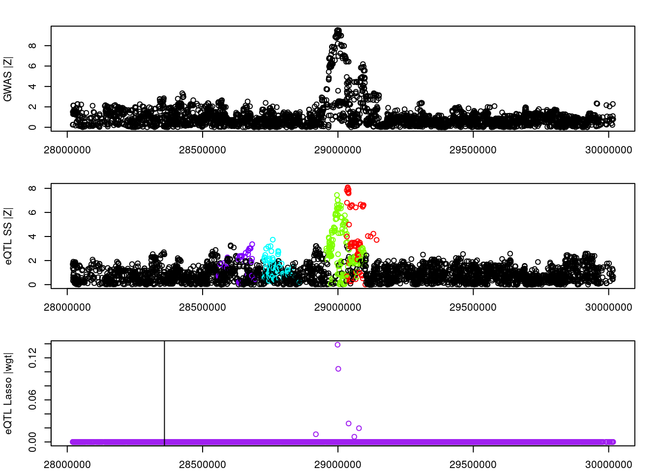

Past versions of unnamed-chunk-6-1.png

Version	Author	Date
d17186e	wesleycrouse	2023-06-08
7f6fbc8	wesleycrouse	2023-05-15
3e493c9	wesleycrouse	2023-05-15

####################

# #load LD matrix for SNPs in all clumps
# snplist_all <- unlist(clumps)
# 
# ld_R_idx <- unique(ld_R_info$index[match(snplist_all, ld_R_info$id)])
# 
# R_snp <- lapply(ld_R_files[ld_R_idx], readRDS)
# 
# R_snp_info <- lapply(ld_R_info_files[ld_R_idx], fread)
# R_snp_info <- lapply(R_snp_info, as.data.frame)
# 
# R_snp_index <- lapply(R_snp_info, function(x){x$id %in% snplist_all})
# rm(snplist_all)
# 
# for (j in 1:length(R_snp)){
#   R_snp[[j]] <- R_snp[[j]][R_snp_index[[j]],R_snp_index[[j]]]
#   R_snp_info[[j]] <- R_snp_info[[j]][R_snp_index[[j]],,drop=F]
# }
# 
# R_snp_info <- as.data.frame(do.call(rbind, R_snp_info))
# R_snp <- as.matrix(Matrix::bdiag(R_snp))
# 
# colnames(R_snp) <- R_snp_info$id
# rownames(R_snp) <- R_snp_info$id
# 
# 
# 
# R_snp_bkup <- R_snp

####################
#load genotypes and compute LD matrix for SNPs in all clumps
snplist_all <- unlist(clumps)

ld_pvarf <- ld_pvarfs[chr]
ldref_file <- ldref_files[chr]

R_snp_info <- read_pvar(ld_pvarf)
ld_pgen <- prep_pgen(pgenf = ldref_file, ld_pvarf)

sidx <- match(snplist_all, R_snp_info$id)
X.g <- read_pgen(ld_pgen, variantidx = sidx)

R_snp <- Rfast::cora(X.g)
colnames(R_snp) <- snplist_all
rownames(R_snp) <- snplist_all

rm(snplist_all, X.g)

####################

#prepare data object
data <- list(sum_stat=list(),
             ld_mat=list())

for (j in 1:length(clumps)){
  snplist <- clumps[[j]]

  R_snp_current <- R_snp[snplist,snplist,drop=F]
  dimnames(R_snp_current) <- NULL

  R_snp_info_current <- R_snp_info[match(snplist, R_snp_info$id),c("id", "ref", "alt")]

  sumstats_current <- data.frame(id=snplist,
                                 ref=R_snp_info_current$ref,
                                 eff=R_snp_info_current$alt,
                                 beta_hat_eqtl=eqtl_current$slope[match(snplist, eqtl_current$SNP)],
                                 beta_hat_gwas=gwas$Estimate[match(snplist, gwas$id)],
                                 se_eqtl=eqtl_current$slope_se[match(snplist, eqtl_current$SNP)],
                                 se_gwas=gwas$Std.Error[match(snplist, gwas$id)])
  sumstats_current$abs_z <- abs(sumstats_current$beta_hat_eqtl/sumstats_current$se_eqtl)

  data$sum_stat[[j]] <- sumstats_current
  data$ld_mat[[j]] <- R_snp_current
}

par(mfrow=c(1,1))

#collapse high correlation SNP keeping most extreme z score (most significant)
data <- collapseHighCorSNPs(data$sum_stat,
                            data$ld_mat,
                            score="abs_z",
                            plot=F)

pre:  71,211,90,48

post: 21,50,48,19

data <- flipAllelesAndGather(data$sum_stat,
                             data$ld_mat,
                             snp_id="id",
                             ref="ref",
                             a="eqtl",
                             sep="_",
                             b="gwas",
                             eff="eff",
                             beta="beta_hat",
                             se="se",
                             a2_plink="ref_eqtl",
                             alleles_same=T)

Past versions of unnamed-chunk-6-2.png

Version	Author	Date
d17186e	wesleycrouse	2023-06-08
7f6fbc8	wesleycrouse	2023-05-15
3e493c9	wesleycrouse	2023-05-15

#colocalization
coloc_fit <- list()
nclust <- length(data$beta_hat_a)

options(mc.cores=4)
for (j in 1:nclust) {
  if (length(data$beta_hat_a[[j]])>1){
    coloc_fit[[j]] <- with(data,
                           fitBetaColoc(
                             beta_hat_a = beta_hat_a[[j]],
                             beta_hat_b = beta_hat_b[[j]],
                             se_a = se_a[[j]],
                             se_b = se_b[[j]],
                             Sigma_a = Sigma[[j]],
                             Sigma_b = Sigma[[j]]
                           ))
  } else {
    coloc_fit[[j]] <- list(beta_hat_a=data$beta_hat_a[[j]],
                           beta_hat_b=data$beta_hat_b[[j]])
  }
}

Warning: There were 538 divergent transitions after warmup. See
https://mc-stan.org/misc/warnings.html#divergent-transitions-after-warmup
to find out why this is a problem and how to eliminate them.

Warning: There were 21 transitions after warmup that exceeded the maximum treedepth. Increase max_treedepth above 10. See
https://mc-stan.org/misc/warnings.html#maximum-treedepth-exceeded

Warning: Examine the pairs() plot to diagnose sampling problems

Warning: Bulk Effective Samples Size (ESS) is too low, indicating posterior means and medians may be unreliable.
Running the chains for more iterations may help. See
https://mc-stan.org/misc/warnings.html#bulk-ess

Warning: Tail Effective Samples Size (ESS) is too low, indicating posterior variances and tail quantiles may be unreliable.
Running the chains for more iterations may help. See
https://mc-stan.org/misc/warnings.html#tail-ess

Warning: There were 518 divergent transitions after warmup. See
https://mc-stan.org/misc/warnings.html#divergent-transitions-after-warmup
to find out why this is a problem and how to eliminate them.

Warning: There were 2805 transitions after warmup that exceeded the maximum treedepth. Increase max_treedepth above 10. See
https://mc-stan.org/misc/warnings.html#maximum-treedepth-exceeded

Warning: There were 4 chains where the estimated Bayesian Fraction of Missing Information was low. See
https://mc-stan.org/misc/warnings.html#bfmi-low

Warning: Examine the pairs() plot to diagnose sampling problems

Warning: The largest R-hat is 1.08, indicating chains have not mixed.
Running the chains for more iterations may help. See
https://mc-stan.org/misc/warnings.html#r-hat

Warning: Bulk Effective Samples Size (ESS) is too low, indicating posterior means and medians may be unreliable.
Running the chains for more iterations may help. See
https://mc-stan.org/misc/warnings.html#bulk-ess

Warning: Tail Effective Samples Size (ESS) is too low, indicating posterior variances and tail quantiles may be unreliable.
Running the chains for more iterations may help. See
https://mc-stan.org/misc/warnings.html#tail-ess

Warning: There were 862 divergent transitions after warmup. See
https://mc-stan.org/misc/warnings.html#divergent-transitions-after-warmup
to find out why this is a problem and how to eliminate them.

Warning: There were 2474 transitions after warmup that exceeded the maximum treedepth. Increase max_treedepth above 10. See
https://mc-stan.org/misc/warnings.html#maximum-treedepth-exceeded

Warning: There were 4 chains where the estimated Bayesian Fraction of Missing Information was low. See
https://mc-stan.org/misc/warnings.html#bfmi-low

Warning: Examine the pairs() plot to diagnose sampling problems

Warning: The largest R-hat is 1.09, indicating chains have not mixed.
Running the chains for more iterations may help. See
https://mc-stan.org/misc/warnings.html#r-hat

Warning: Bulk Effective Samples Size (ESS) is too low, indicating posterior means and medians may be unreliable.
Running the chains for more iterations may help. See
https://mc-stan.org/misc/warnings.html#bulk-ess

Warning: Tail Effective Samples Size (ESS) is too low, indicating posterior variances and tail quantiles may be unreliable.
Running the chains for more iterations may help. See
https://mc-stan.org/misc/warnings.html#tail-ess

Warning: There were 656 divergent transitions after warmup. See
https://mc-stan.org/misc/warnings.html#divergent-transitions-after-warmup
to find out why this is a problem and how to eliminate them.

Warning: There were 634 transitions after warmup that exceeded the maximum treedepth. Increase max_treedepth above 10. See
https://mc-stan.org/misc/warnings.html#maximum-treedepth-exceeded

Warning: There were 3 chains where the estimated Bayesian Fraction of Missing Information was low. See
https://mc-stan.org/misc/warnings.html#bfmi-low

Warning: Examine the pairs() plot to diagnose sampling problems

Warning: The largest R-hat is 1.07, indicating chains have not mixed.
Running the chains for more iterations may help. See
https://mc-stan.org/misc/warnings.html#r-hat

Warning: Bulk Effective Samples Size (ESS) is too low, indicating posterior means and medians may be unreliable.
Running the chains for more iterations may help. See
https://mc-stan.org/misc/warnings.html#bulk-ess

Warning: Tail Effective Samples Size (ESS) is too low, indicating posterior variances and tail quantiles may be unreliable.
Running the chains for more iterations may help. See
https://mc-stan.org/misc/warnings.html#tail-ess

res <- list(beta_hat_a = lapply(coloc_fit, `[[`, "beta_hat_a"),
            beta_hat_b = lapply(coloc_fit, `[[`, "beta_hat_b"),
            sd_a = data$se_a,
            sd_b = data$se_b,
            alleles = data$alleles)

res <- extractForSlope(res)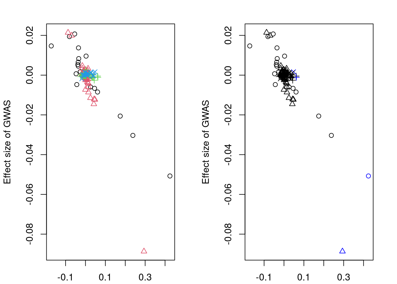

Past versions of unnamed-chunk-6-3.png

Version	Author	Date
d17186e	wesleycrouse	2023-06-08
7f6fbc8	wesleycrouse	2023-05-15
3e493c9	wesleycrouse	2023-05-15

res

$beta_hat_a
[1] 0.42455854 0.29397084 0.06234380 0.04789981

$beta_hat_b
[1] -0.050738650 -0.088684800 -0.001114566  0.001667316

$sd_a
[1] 0.0787349 0.0476176 0.0609834 0.0808790

$sd_b
[1] 0.01665773 0.01042285 0.01254851 0.01625646

$alleles
            id ref eff
1   rs11978975   C   T
22   rs1006521   G   A
90  rs12533079   T   G
130 rs73081813   T   C

#sort clusters by significance
res$abs_z <- abs(res$beta_hat_a/res$sd_a)
res_sig_order <- order(-res$abs_z)

res$beta_hat_a <- res$beta_hat_a[res_sig_order]
res$beta_hat_b <- res$beta_hat_b[res_sig_order]
res$sd_a <- res$sd_a[res_sig_order]
res$sd_b <- res$sd_b[res_sig_order]
res$alleles <- res$alleles[res_sig_order,,drop=F]
res$abs_z <- NULL

####################

res_bkup <- res

####################

#trim clusters if (absolute) correlation greater than 0.05
if (length(res$alleles$id)>1){
  trim_index <- trimClusters(r2=abs(R_snp[res$alleles$id,res$alleles$id,drop=F]),
                             r2_threshold=0.05)

  if (length(trim_index)>0){
    res$beta_hat_a <- res$beta_hat_a[-trim_index]
    res$beta_hat_b <- res$beta_hat_b[-trim_index]
    res$sd_a <- res$sd_a[-trim_index]
    res$sd_b <- res$sd_b[-trim_index]
    res$alleles <- res$alleles[-trim_index,,drop=F]
  }
}

####################
#visual input data

par(mfrow=c(3,1))

logging::loginfo(gene)

2023-06-12 15:30:15 INFO::ENSG00000272568

par(mar=c(2.1, 4.1, 2.1, 2.1))

plot(df_locus$pos, abs(df_locus$z_gwas), xlab="", ylab="GWAS |Z|")
abline(v=df_locus$pos[df_locus$causal], col="red")

plot(df_locus$pos, abs(df_locus$z_eqtl), xlab="", ylab="eQTL SS |Z|",
     col=colors[df_locus$clump+1])
abline(v=df_locus$pos[df_locus$causal], col="red")

plot(df_locus$pos, abs(df_locus$weight), col="purple", xlab="", ylab="eQTL Lasso |wgt|")
abline(v=df_locus$pos[df_locus$causal], col="red")

breakpoints <- ld_R_info[ld_R_info$index!=c(ld_R_info$index[-1],max(ld_R_info$index)),]
breakpoints <- breakpoints[breakpoints$chrom==chr,]
breakpoints <- breakpoints[breakpoints$pos>min(df_locus$pos) & breakpoints$pos<max(df_locus$pos),]

abline(v=breakpoints$pos)

Past versions of unnamed-chunk-6-4.png

Version	Author	Date
d17186e	wesleycrouse	2023-06-08

df_locus$trim <- F
df_locus$trim[match(res_bkup$alleles$id[trim_index], df_locus$id)] <- T
df_locus$color <- colors[df_locus$clump+1]
df_locus[match(res_bkup$alleles$id, df_locus$id),]

                id    z_eqtl chrom      pos     z_gwas causal weight clump
5438240  rs1006521 -7.447246     7 28996220  9.4682753  FALSE      0     2
5438362 rs11978975 -8.080584     7 29036108  4.4252724  FALSE      0     1
5437670 rs12533079 -3.201658     7 28751137  0.9224921  FALSE      0     3
5437448 rs73081813 -2.636321     7 28659030 -0.7916247  FALSE      0     4
         trim   color
5438240 FALSE #80FF00
5438362  TRUE #FF0000
5437670  TRUE #00FFFF
5437448 FALSE #8000FF

par(mfrow=c(1,1))

scales::show_col(colors[c(1, res_sig_order+1)])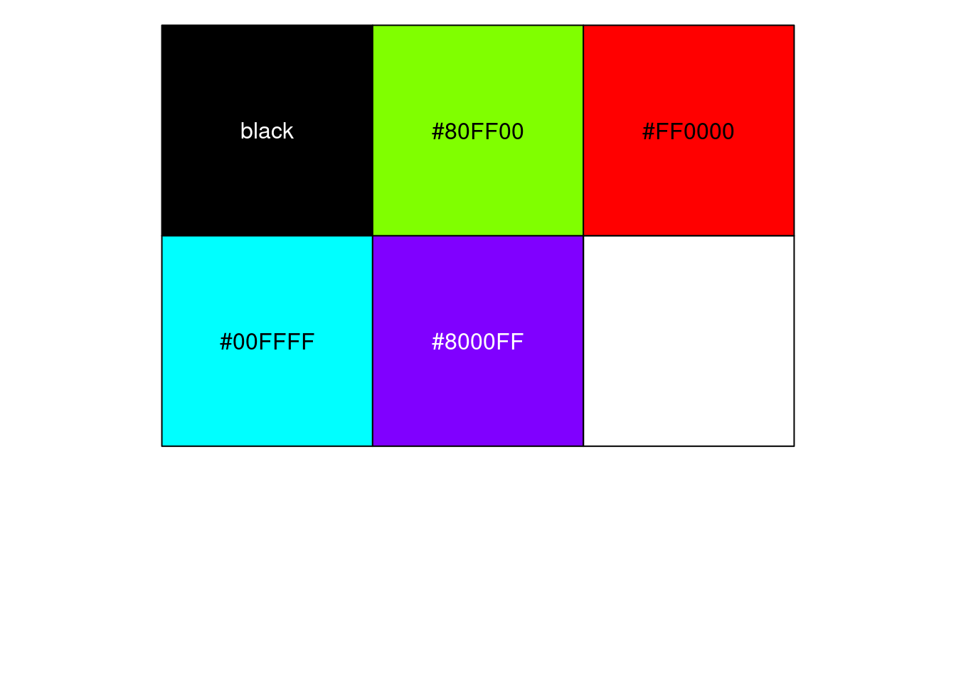

Past versions of unnamed-chunk-6-5.png

Version	Author	Date
d17186e	wesleycrouse	2023-06-08

####################

if (length(res$beta_hat_a)==1){
  #parametric sample from MRLocus code
  m <- 1e+05
  post_samples <- list(alpha=rnorm(m, res$beta_hat_b, res$sd_b)/rnorm(m, res$beta_hat_a, res$sd_a))
} else {
  #fit MRLocus slope model
  res <- fitSlope(res, iter=10000)
  post_samples <- rstan::extract(res$stanfit)
}

Warning: There were 2317 divergent transitions after warmup. See
https://mc-stan.org/misc/warnings.html#divergent-transitions-after-warmup
to find out why this is a problem and how to eliminate them.

Warning: Examine the pairs() plot to diagnose sampling problems

Warning: Bulk Effective Samples Size (ESS) is too low, indicating posterior means and medians may be unreliable.
Running the chains for more iterations may help. See
https://mc-stan.org/misc/warnings.html#bulk-ess

Warning: Tail Effective Samples Size (ESS) is too low, indicating posterior variances and tail quantiles may be unreliable.
Running the chains for more iterations may help. See
https://mc-stan.org/misc/warnings.html#tail-ess

par(mfrow=c(1,1))

#display results
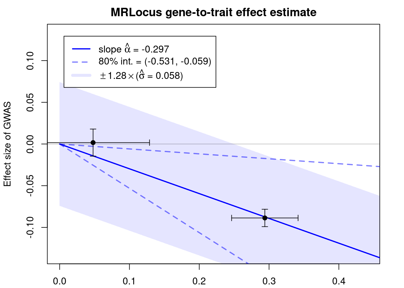
print(res$stanfit, pars=c("alpha","sigma"), probs=c(.1,.9), digits=3)

Inference for Stan model: slope.
4 chains, each with iter=10000; warmup=5000; thin=1; 
post-warmup draws per chain=5000, total post-warmup draws=20000.

        mean se_mean    sd    10%    90% n_eff  Rhat
alpha -0.297   0.003 0.221 -0.531 -0.059  7275 1.000
sigma  0.058   0.001 0.052  0.009  0.130  1309 1.005

Samples were drawn using NUTS(diag_e) at Mon Jun 12 15:30:17 2023.
For each parameter, n_eff is a crude measure of effective sample size,
and Rhat is the potential scale reduction factor on split chains (at 
convergence, Rhat=1).

if (!is.null(res$stanfit)){
  plotMrlocus(res, main="MRLocus gene-to-trait effect estimate")
} else {
  logging::loginfo("<2 clumps for analysis")
}

Past versions of unnamed-chunk-6-6.png

Version	Author	Date
d17186e	wesleycrouse	2023-06-08

False positives

ENSG00000243335

set.seed(4099)

load("/home/wcrouse/scratch-midway2/mrlocus_image.RData")

####################
#run MR-Locus 

gene <- "ENSG00000243335"

chr <- as.numeric(gtf_df$seqnames[gtf_df$gene_id==gene])

#prepare files for plink
plink_exclude_file <- paste0(temp_dir, "ukb_chr", chr, "_s80.45.2.exclude")

if (!file.exists(plink_exclude_file)){
  #store list of SNPs in .bed file using plink
  system_cmd <- paste0("plink --bfile ",
                       ld_bedfs$file[chr],
                       " --write-snplist --out ",
                       temp_dir, "ukb_chr", chr, "_s80.45.2")
  system(system_cmd)

  #store list of duplicate SNPs in .bed file to exclude
  system_cmd <- paste0("sort ",
                       temp_dir,
                       "ukb_chr", chr, "_s80.45.2.snplist|uniq -d > ",
                       temp_dir,
                       "ukb_chr", chr, "_s80.45.2.exclude")

  system(system_cmd)
}

#clumping using plink
eqtl_current <- eqtl[eqtl$gene_id==gene,]
eqtl_current <- dplyr::rename(eqtl_current, SNP="id", P="pval_nominal")

eqtl_current_file <- paste0(temp_dir, outname_base, ".eqtl_sumstats.", gene, ".temp")
write.table(eqtl_current, file=eqtl_current_file, sep="\t", col.names=T, row.names=F, quote=F)

eqtl_clump_file <- paste0(temp_dir, outname_base, ".eqtl_clumps.", gene, ".temp")
system_cmd <- paste0("plink --bfile ",
                     ld_bedfs$file[chr],
                     " --clump ",
                     eqtl_current_file,
                     " --clump-p1 0.001 --clump-p2 1 --clump-r2 0.1 --clump-kb 500 --out ",
                     eqtl_clump_file,
                     " --exclude ",
                     plink_exclude_file)

#system(system_cmd)
print(system_cmd)

[1] "plink --bfile /home/wcrouse/causalTWAS/simulations/simulation_ctwas_rss_20210416_compare/ukb_chr7_s80.45.2.FUSION7 --clump /home/wcrouse/causalTWAS/simulations/simulation_ctwas_rss_20210416_compare/temp_mrlocus/mrlocus_report_temp.eqtl_sumstats.ENSG00000243335.temp --clump-p1 0.001 --clump-p2 1 --clump-r2 0.1 --clump-kb 500 --out /home/wcrouse/causalTWAS/simulations/simulation_ctwas_rss_20210416_compare/temp_mrlocus/mrlocus_report_temp.eqtl_clumps.ENSG00000243335.temp --exclude /home/wcrouse/causalTWAS/simulations/simulation_ctwas_rss_20210416_compare/temp_mrlocus/ukb_chr7_s80.45.2.exclude"

eqtl_clump_file <- paste0(eqtl_clump_file, ".clumped")

clumps <- read.table(eqtl_clump_file, header=T)
clumps$SP2 <- sapply(1:nrow(clumps), function(x){paste0(clumps$SNP[x], "(1),", clumps$SP2[x])})
clumps <- lapply(clumps$SP2, function(y){unname(sapply(unlist(strsplit(y, ",")), function(x){unlist(strsplit(x, "[(]"))[1]}))})
clumps <- lapply(clumps, function(x){x[x!="NONE"]})

####################

df_locus <- data.frame(id=eqtl_current$SNP, z_eqtl=eqtl_current$slope/eqtl_current$slope_se)
df_locus <- cbind(df_locus, ld_R_info[match(df_locus$id, ld_R_info$id),c("chrom","pos")])
df_locus$z_gwas <- (gwas$Estimate/gwas$Std.Error)[match(df_locus$id, gwas$id)]
df_locus$causal <- df_locus$id %in% names(true_snp_effects) 

weightf_dir <- "/project2/mstephens/causalTWAS/fusion_weights/Adipose_Subcutaneous/"
weightf_gene <- list.files(weightf_dir)
weightf_gene <- paste0(weightf_dir, weightf_gene[grep(gene, weightf_gene)])
load(weightf_gene)

df_locus$weight <- wgt.matrix[match(df_locus$id, rownames(wgt.matrix)),"lasso"]
df_locus$weight[is.na(df_locus$weight)] <- 0

df_locus$clump <- 0

for (j in 1:length(clumps)){
  df_locus$clump[df_locus$id %in% clumps[[j]]] <- j
}

#visualize input data
colors <- c("black", rainbow(length(clumps)))

par(mfrow=c(3,1))

logging::loginfo(gene)

2023-06-12 15:30:59 INFO::ENSG00000243335

par(mar=c(2.1, 4.1, 2.1, 2.1))

plot(df_locus$pos, abs(df_locus$z_gwas), xlab="", ylab="GWAS |Z|")
abline(v=df_locus$pos[df_locus$causal], col="red")

plot(df_locus$pos, abs(df_locus$z_eqtl), xlab="", ylab="eQTL SS |Z|",
     col=colors[df_locus$clump+1])
abline(v=df_locus$pos[df_locus$causal], col="red")

plot(df_locus$pos, abs(df_locus$weight), col="purple", xlab="", ylab="eQTL Lasso |wgt|")
abline(v=df_locus$pos[df_locus$causal], col="red")

breakpoints <- ld_R_info[ld_R_info$index!=c(ld_R_info$index[-1],max(ld_R_info$index)),]
breakpoints <- breakpoints[breakpoints$chrom==chr,]
breakpoints <- breakpoints[breakpoints$pos>min(df_locus$pos) & breakpoints$pos<max(df_locus$pos),]

abline(v=breakpoints$pos)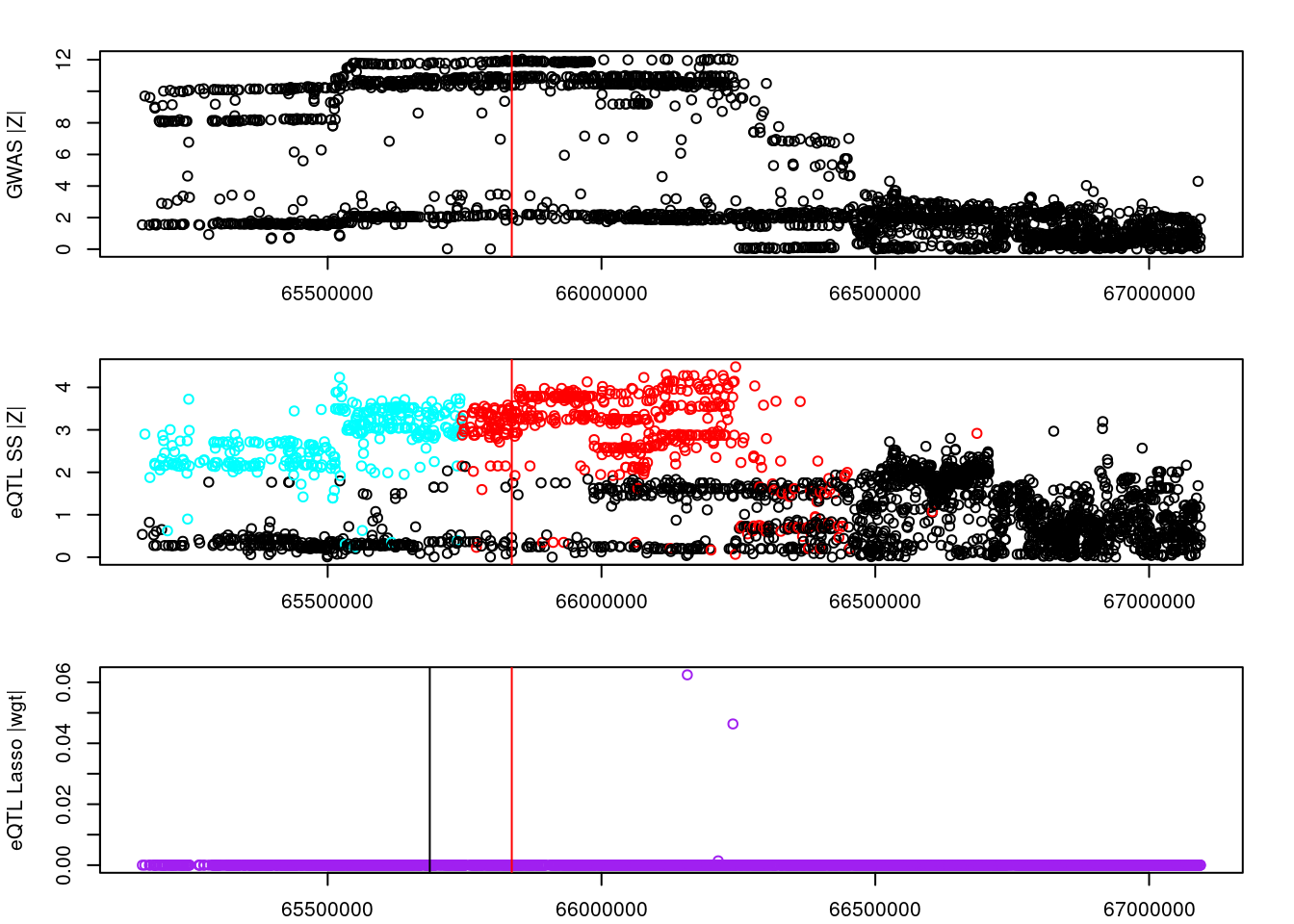

Past versions of unnamed-chunk-7-1.png

Version	Author	Date
d17186e	wesleycrouse	2023-06-08
3e493c9	wesleycrouse	2023-05-15

####################

# #load LD matrix for SNPs in all clumps
# snplist_all <- unlist(clumps)
# 
# ld_R_idx <- unique(ld_R_info$index[match(snplist_all, ld_R_info$id)])
# 
# R_snp <- lapply(ld_R_files[ld_R_idx], readRDS)
# 
# R_snp_info <- lapply(ld_R_info_files[ld_R_idx], fread)
# R_snp_info <- lapply(R_snp_info, as.data.frame)
# 
# R_snp_index <- lapply(R_snp_info, function(x){x$id %in% snplist_all})
# rm(snplist_all)
# 
# for (j in 1:length(R_snp)){
#   R_snp[[j]] <- R_snp[[j]][R_snp_index[[j]],R_snp_index[[j]]]
#   R_snp_info[[j]] <- R_snp_info[[j]][R_snp_index[[j]],,drop=F]
# }
# 
# R_snp_info <- as.data.frame(do.call(rbind, R_snp_info))
# R_snp <- as.matrix(Matrix::bdiag(R_snp))
# 
# colnames(R_snp) <- R_snp_info$id
# rownames(R_snp) <- R_snp_info$id
# 
# 
# 
# R_snp_bkup <- R_snp

####################
#load genotypes and compute LD matrix for SNPs in all clumps
snplist_all <- unlist(clumps)

ld_pvarf <- ld_pvarfs[chr]
ldref_file <- ldref_files[chr]

R_snp_info <- read_pvar(ld_pvarf)
ld_pgen <- prep_pgen(pgenf = ldref_file, ld_pvarf)

sidx <- match(snplist_all, R_snp_info$id)
X.g <- read_pgen(ld_pgen, variantidx = sidx)

R_snp <- Rfast::cora(X.g)
colnames(R_snp) <- snplist_all
rownames(R_snp) <- snplist_all

rm(snplist_all, X.g)

####################

#prepare data object
data <- list(sum_stat=list(),
             ld_mat=list())

for (j in 1:length(clumps)){
  snplist <- clumps[[j]]

  R_snp_current <- R_snp[snplist,snplist,drop=F]
  dimnames(R_snp_current) <- NULL

  R_snp_info_current <- R_snp_info[match(snplist, R_snp_info$id),c("id", "ref", "alt")]

  sumstats_current <- data.frame(id=snplist,
                                 ref=R_snp_info_current$ref,
                                 eff=R_snp_info_current$alt,
                                 beta_hat_eqtl=eqtl_current$slope[match(snplist, eqtl_current$SNP)],
                                 beta_hat_gwas=gwas$Estimate[match(snplist, gwas$id)],
                                 se_eqtl=eqtl_current$slope_se[match(snplist, eqtl_current$SNP)],
                                 se_gwas=gwas$Std.Error[match(snplist, gwas$id)])
  sumstats_current$abs_z <- abs(sumstats_current$beta_hat_eqtl/sumstats_current$se_eqtl)

  data$sum_stat[[j]] <- sumstats_current
  data$ld_mat[[j]] <- R_snp_current
}

par(mfrow=c(1,1))

#collapse high correlation SNP keeping most extreme z score (most significant)
data <- collapseHighCorSNPs(data$sum_stat,
                            data$ld_mat,
                            score="abs_z",
                            plot=F)

pre:  541,338

post: 37,28

data <- flipAllelesAndGather(data$sum_stat,
                             data$ld_mat,
                             snp_id="id",
                             ref="ref",
                             a="eqtl",
                             sep="_",
                             b="gwas",
                             eff="eff",
                             beta="beta_hat",
                             se="se",
                             a2_plink="ref_eqtl",
                             alleles_same=T)

Past versions of unnamed-chunk-7-2.png

Version	Author	Date
d17186e	wesleycrouse	2023-06-08
7f6fbc8	wesleycrouse	2023-05-15
3e493c9	wesleycrouse	2023-05-15

#colocalization
coloc_fit <- list()
nclust <- length(data$beta_hat_a)

options(mc.cores=4)
for (j in 1:nclust) {
  if (length(data$beta_hat_a[[j]])>1){
    coloc_fit[[j]] <- with(data,
                           fitBetaColoc(
                             beta_hat_a = beta_hat_a[[j]],
                             beta_hat_b = beta_hat_b[[j]],
                             se_a = se_a[[j]],
                             se_b = se_b[[j]],
                             Sigma_a = Sigma[[j]],
                             Sigma_b = Sigma[[j]]
                           ))
  } else {
    coloc_fit[[j]] <- list(beta_hat_a=data$beta_hat_a[[j]],
                           beta_hat_b=data$beta_hat_b[[j]])
  }
}

Warning: There were 775 divergent transitions after warmup. See
https://mc-stan.org/misc/warnings.html#divergent-transitions-after-warmup
to find out why this is a problem and how to eliminate them.

Warning: There were 1209 transitions after warmup that exceeded the maximum treedepth. Increase max_treedepth above 10. See
https://mc-stan.org/misc/warnings.html#maximum-treedepth-exceeded

Warning: There were 3 chains where the estimated Bayesian Fraction of Missing Information was low. See
https://mc-stan.org/misc/warnings.html#bfmi-low

Warning: Examine the pairs() plot to diagnose sampling problems

Warning: The largest R-hat is 1.06, indicating chains have not mixed.
Running the chains for more iterations may help. See
https://mc-stan.org/misc/warnings.html#r-hat

Warning: Bulk Effective Samples Size (ESS) is too low, indicating posterior means and medians may be unreliable.
Running the chains for more iterations may help. See
https://mc-stan.org/misc/warnings.html#bulk-ess

Warning: Tail Effective Samples Size (ESS) is too low, indicating posterior variances and tail quantiles may be unreliable.
Running the chains for more iterations may help. See
https://mc-stan.org/misc/warnings.html#tail-ess

Warning: There were 1760 divergent transitions after warmup. See
https://mc-stan.org/misc/warnings.html#divergent-transitions-after-warmup
to find out why this is a problem and how to eliminate them.

Warning: There were 49 transitions after warmup that exceeded the maximum treedepth. Increase max_treedepth above 10. See
https://mc-stan.org/misc/warnings.html#maximum-treedepth-exceeded

Warning: There were 2 chains where the estimated Bayesian Fraction of Missing Information was low. See
https://mc-stan.org/misc/warnings.html#bfmi-low

Warning: Examine the pairs() plot to diagnose sampling problems

Warning: The largest R-hat is 1.6, indicating chains have not mixed.
Running the chains for more iterations may help. See
https://mc-stan.org/misc/warnings.html#r-hat

Warning: Bulk Effective Samples Size (ESS) is too low, indicating posterior means and medians may be unreliable.
Running the chains for more iterations may help. See
https://mc-stan.org/misc/warnings.html#bulk-ess

Warning: Tail Effective Samples Size (ESS) is too low, indicating posterior variances and tail quantiles may be unreliable.
Running the chains for more iterations may help. See
https://mc-stan.org/misc/warnings.html#tail-ess

res <- list(beta_hat_a = lapply(coloc_fit, `[[`, "beta_hat_a"),
            beta_hat_b = lapply(coloc_fit, `[[`, "beta_hat_b"),
            sd_a = data$se_a,
            sd_b = data$se_b,
            alleles = data$alleles)

res <- extractForSlope(res)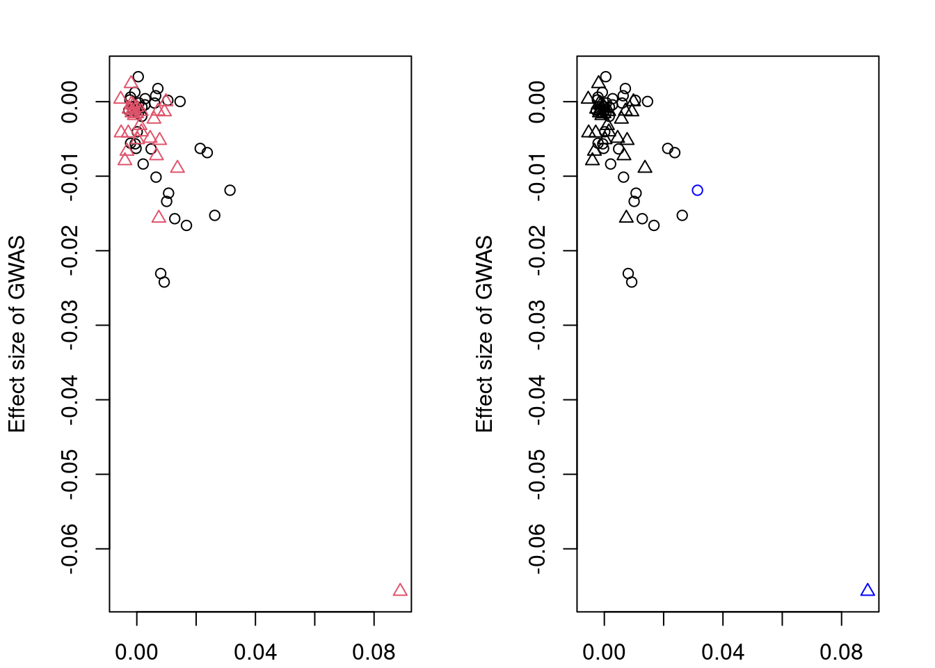

Past versions of unnamed-chunk-7-3.png

Version	Author	Date
d17186e	wesleycrouse	2023-06-08
7f6fbc8	wesleycrouse	2023-05-15
3e493c9	wesleycrouse	2023-05-15

res

$beta_hat_a
[1] 0.03141847 0.08881357

$beta_hat_b
[1] -0.01188617 -0.06570110

$sd_a
[1] 0.0582605 0.0303630

$sd_b
[1] 0.01968043 0.01070247

$alleles
            id ref eff
2  rs116950228   G   A
60    rs313829   G   A

#sort clusters by significance
res$abs_z <- abs(res$beta_hat_a/res$sd_a)
res_sig_order <- order(-res$abs_z)

res$beta_hat_a <- res$beta_hat_a[res_sig_order]
res$beta_hat_b <- res$beta_hat_b[res_sig_order]
res$sd_a <- res$sd_a[res_sig_order]
res$sd_b <- res$sd_b[res_sig_order]
res$alleles <- res$alleles[res_sig_order,,drop=F]
res$abs_z <- NULL

####################

res_bkup <- res

####################

#trim clusters if (absolute) correlation greater than 0.05
if (length(res$alleles$id)>1){
  trim_index <- trimClusters(r2=abs(R_snp[res$alleles$id,res$alleles$id,drop=F]),
                             r2_threshold=0.05)

  if (length(trim_index)>0){
    res$beta_hat_a <- res$beta_hat_a[-trim_index]
    res$beta_hat_b <- res$beta_hat_b[-trim_index]
    res$sd_a <- res$sd_a[-trim_index]
    res$sd_b <- res$sd_b[-trim_index]
    res$alleles <- res$alleles[-trim_index,,drop=F]
  }
}

####################
#visual input data

par(mfrow=c(3,1))

logging::loginfo(gene)

2023-06-12 15:32:10 INFO::ENSG00000243335

par(mar=c(2.1, 4.1, 2.1, 2.1))

plot(df_locus$pos, abs(df_locus$z_gwas), xlab="", ylab="GWAS |Z|")
abline(v=df_locus$pos[df_locus$causal], col="red")

plot(df_locus$pos, abs(df_locus$z_eqtl), xlab="", ylab="eQTL SS |Z|",
     col=colors[df_locus$clump+1])
abline(v=df_locus$pos[df_locus$causal], col="red")

plot(df_locus$pos, abs(df_locus$weight), col="purple", xlab="", ylab="eQTL Lasso |wgt|")
abline(v=df_locus$pos[df_locus$causal], col="red")

breakpoints <- ld_R_info[ld_R_info$index!=c(ld_R_info$index[-1],max(ld_R_info$index)),]
breakpoints <- breakpoints[breakpoints$chrom==chr,]
breakpoints <- breakpoints[breakpoints$pos>min(df_locus$pos) & breakpoints$pos<max(df_locus$pos),]

abline(v=breakpoints$pos)

Past versions of unnamed-chunk-7-4.png

Version	Author	Date
d17186e	wesleycrouse	2023-06-08
7f6fbc8	wesleycrouse	2023-05-15

df_locus$trim <- F
df_locus$trim[match(res_bkup$alleles$id[trim_index], df_locus$id)] <- T
df_locus$color <- colors[df_locus$clump+1]
df_locus[match(res_bkup$alleles$id, df_locus$id),]

                 id    z_eqtl chrom      pos     z_gwas causal weight clump
5526879    rs313829  3.604848     7 65552497 -11.236654  FALSE      0     2
5528331 rs116950228 -2.264399     7 66327084   3.590381  FALSE      0     1
         trim   color
5526879 FALSE #00FFFF
5528331  TRUE #FF0000

par(mfrow=c(1,1))

scales::show_col(colors[c(1, res_sig_order+1)])

Past versions of unnamed-chunk-7-5.png

Version	Author	Date
d17186e	wesleycrouse	2023-06-08

####################

if (length(res$beta_hat_a)==1){
  #parametric sample from MRLocus code
  m <- 1e+05
  post_samples <- list(alpha=rnorm(m, res$beta_hat_b, res$sd_b)/rnorm(m, res$beta_hat_a, res$sd_a))
} else {
  #fit MRLocus slope model
  res <- fitSlope(res, iter=10000)
  post_samples <- rstan::extract(res$stanfit)
}

par(mfrow=c(1,1))

#display results
print(res$stanfit, pars=c("alpha","sigma"), probs=c(.1,.9), digits=3)

NULL

if (!is.null(res$stanfit)){
  plotMrlocus(res, main="MRLocus gene-to-trait effect estimate")
} else {
  logging::loginfo("<2 clumps for analysis")
}

2023-06-12 15:32:11 INFO::<2 clumps for analysis

####################
#investigate LD between confounding variants and eSNPs for clumps

#confounding causal SNPs
df_locus[df_locus$causal,]

              id    z_eqtl chrom      pos   z_gwas causal weight clump  trim
5527360 rs778685 -3.392917     7 65836176 11.90402   TRUE      0     1 FALSE
          color
5527360 #FF0000

#eSNPs in the analysis
df_locus[match(res$alleles$id, df_locus$id),]

              id   z_eqtl chrom      pos    z_gwas causal weight clump  trim
5526879 rs313829 3.604848     7 65552497 -11.23665  FALSE      0     2 FALSE
          color
5526879 #00FFFF

#LD between confounding SNPs and eSNPs
snplist_all <- c(df_locus$id[df_locus$causal], res$alleles$id)

ld_R_idx <- unique(ld_R_info$index[match(snplist_all, ld_R_info$id)])

R_snp <- lapply(ld_R_files[ld_R_idx], readRDS)

R_snp_info <- lapply(ld_R_info_files[ld_R_idx], fread)
R_snp_info <- lapply(R_snp_info, as.data.frame)

R_snp_index <- lapply(R_snp_info, function(x){x$id %in% snplist_all})

for (j in 1:length(R_snp)){
  R_snp[[j]] <- R_snp[[j]][R_snp_index[[j]],R_snp_index[[j]]]
  R_snp_info[[j]] <- R_snp_info[[j]][R_snp_index[[j]],,drop=F]
}

R_snp_info <- as.data.frame(do.call(rbind, R_snp_info))
R_snp <- as.matrix(Matrix::bdiag(R_snp))

colnames(R_snp) <- R_snp_info$id
rownames(R_snp) <- R_snp_info$id

#number of LD regions
length(ld_R_idx)

[1] 2

#LD between variants
R_snp[snplist_all, snplist_all]

         rs778685 rs313829
rs778685        1        0
rs313829        0        1

False negatives

ENSG00000215022

set.seed(45102)

load("/home/wcrouse/scratch-midway2/mrlocus_image.RData")

####################
#run MR-Locus 

gene <- "ENSG00000215022"

chr <- as.numeric(gtf_df$seqnames[gtf_df$gene_id==gene])

#prepare files for plink
plink_exclude_file <- paste0(temp_dir, "ukb_chr", chr, "_s80.45.2.exclude")

if (!file.exists(plink_exclude_file)){
  #store list of SNPs in .bed file using plink
  system_cmd <- paste0("plink --bfile ",
                       ld_bedfs$file[chr],
                       " --write-snplist --out ",
                       temp_dir, "ukb_chr", chr, "_s80.45.2")
  system(system_cmd)

  #store list of duplicate SNPs in .bed file to exclude
  system_cmd <- paste0("sort ",
                       temp_dir,
                       "ukb_chr", chr, "_s80.45.2.snplist|uniq -d > ",
                       temp_dir,
                       "ukb_chr", chr, "_s80.45.2.exclude")

  system(system_cmd)
}

#clumping using plink
eqtl_current <- eqtl[eqtl$gene_id==gene,]
eqtl_current <- dplyr::rename(eqtl_current, SNP="id", P="pval_nominal")

eqtl_current_file <- paste0(temp_dir, outname_base, ".eqtl_sumstats.", gene, ".temp")
write.table(eqtl_current, file=eqtl_current_file, sep="\t", col.names=T, row.names=F, quote=F)

eqtl_clump_file <- paste0(temp_dir, outname_base, ".eqtl_clumps.", gene, ".temp")
system_cmd <- paste0("plink --bfile ",
                     ld_bedfs$file[chr],
                     " --clump ",
                     eqtl_current_file,
                     " --clump-p1 0.001 --clump-p2 1 --clump-r2 0.1 --clump-kb 500 --out ",
                     eqtl_clump_file,
                     " --exclude ",
                     plink_exclude_file)

#system(system_cmd)
print(system_cmd)

[1] "plink --bfile /home/wcrouse/causalTWAS/simulations/simulation_ctwas_rss_20210416_compare/ukb_chr6_s80.45.2.FUSION6 --clump /home/wcrouse/causalTWAS/simulations/simulation_ctwas_rss_20210416_compare/temp_mrlocus/mrlocus_report_temp.eqtl_sumstats.ENSG00000215022.temp --clump-p1 0.001 --clump-p2 1 --clump-r2 0.1 --clump-kb 500 --out /home/wcrouse/causalTWAS/simulations/simulation_ctwas_rss_20210416_compare/temp_mrlocus/mrlocus_report_temp.eqtl_clumps.ENSG00000215022.temp --exclude /home/wcrouse/causalTWAS/simulations/simulation_ctwas_rss_20210416_compare/temp_mrlocus/ukb_chr6_s80.45.2.exclude"

eqtl_clump_file <- paste0(eqtl_clump_file, ".clumped")

clumps <- read.table(eqtl_clump_file, header=T)
clumps$SP2 <- sapply(1:nrow(clumps), function(x){paste0(clumps$SNP[x], "(1),", clumps$SP2[x])})
clumps <- lapply(clumps$SP2, function(y){unname(sapply(unlist(strsplit(y, ",")), function(x){unlist(strsplit(x, "[(]"))[1]}))})
clumps <- lapply(clumps, function(x){x[x!="NONE"]})

####################

df_locus <- data.frame(id=eqtl_current$SNP, z_eqtl=eqtl_current$slope/eqtl_current$slope_se)
df_locus <- cbind(df_locus, ld_R_info[match(df_locus$id, ld_R_info$id),c("chrom","pos")])
df_locus$z_gwas <- (gwas$Estimate/gwas$Std.Error)[match(df_locus$id, gwas$id)]
df_locus$causal <- df_locus$id %in% names(true_snp_effects) 

weightf_dir <- "/project2/mstephens/causalTWAS/fusion_weights/Adipose_Subcutaneous/"
weightf_gene <- list.files(weightf_dir)
weightf_gene <- paste0(weightf_dir, weightf_gene[grep(gene, weightf_gene)])
load(weightf_gene)

df_locus$weight <- wgt.matrix[match(df_locus$id, rownames(wgt.matrix)),"lasso"]
df_locus$weight[is.na(df_locus$weight)] <- 0

df_locus$clump <- 0

for (j in 1:length(clumps)){
  df_locus$clump[df_locus$id %in% clumps[[j]]] <- j
}

#visualize input data
colors <- c("black", rainbow(length(clumps)))

par(mfrow=c(3,1))

logging::loginfo(gene)

2023-06-12 15:32:58 INFO::ENSG00000215022

par(mar=c(2.1, 4.1, 2.1, 2.1))

plot(df_locus$pos, abs(df_locus$z_gwas), xlab="", ylab="GWAS |Z|")
abline(v=df_locus$pos[df_locus$causal], col="red")

plot(df_locus$pos, abs(df_locus$z_eqtl), xlab="", ylab="eQTL SS |Z|",
     col=colors[df_locus$clump+1])
abline(v=df_locus$pos[df_locus$causal], col="red")

plot(df_locus$pos, abs(df_locus$weight), col="purple", xlab="", ylab="eQTL Lasso |wgt|")
abline(v=df_locus$pos[df_locus$causal], col="red")

breakpoints <- ld_R_info[ld_R_info$index!=c(ld_R_info$index[-1],max(ld_R_info$index)),]
breakpoints <- breakpoints[breakpoints$chrom==chr,]
breakpoints <- breakpoints[breakpoints$pos>min(df_locus$pos) & breakpoints$pos<max(df_locus$pos),]

abline(v=breakpoints$pos)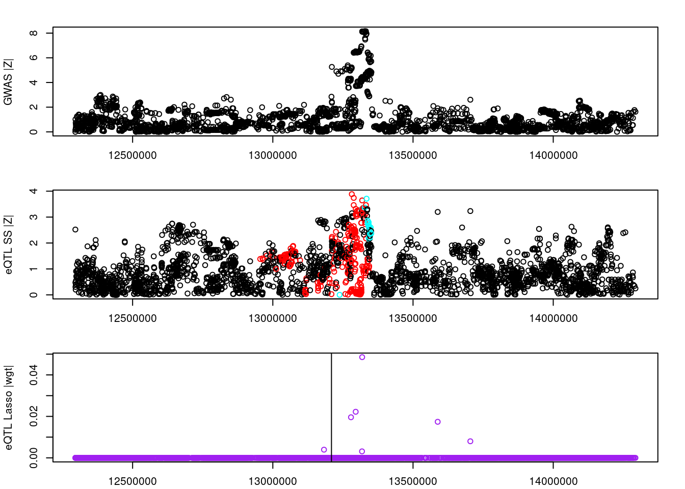

Past versions of unnamed-chunk-8-1.png

Version	Author	Date
d17186e	wesleycrouse	2023-06-08
3e493c9	wesleycrouse	2023-05-15

####################

# #load LD matrix for SNPs in all clumps
# snplist_all <- unlist(clumps)
# 
# ld_R_idx <- unique(ld_R_info$index[match(snplist_all, ld_R_info$id)])
# 
# R_snp <- lapply(ld_R_files[ld_R_idx], readRDS)
# 
# R_snp_info <- lapply(ld_R_info_files[ld_R_idx], fread)
# R_snp_info <- lapply(R_snp_info, as.data.frame)
# 
# R_snp_index <- lapply(R_snp_info, function(x){x$id %in% snplist_all})
# rm(snplist_all)
# 
# for (j in 1:length(R_snp)){
#   R_snp[[j]] <- R_snp[[j]][R_snp_index[[j]],R_snp_index[[j]]]
#   R_snp_info[[j]] <- R_snp_info[[j]][R_snp_index[[j]],,drop=F]
# }
# 
# R_snp_info <- as.data.frame(do.call(rbind, R_snp_info))
# R_snp <- as.matrix(Matrix::bdiag(R_snp))
# 
# colnames(R_snp) <- R_snp_info$id
# rownames(R_snp) <- R_snp_info$id
# 
# 
# 
# R_snp_bkup <- R_snp

####################
#load genotypes and compute LD matrix for SNPs in all clumps
snplist_all <- unlist(clumps)

ld_pvarf <- ld_pvarfs[chr]
ldref_file <- ldref_files[chr]

R_snp_info <- read_pvar(ld_pvarf)
ld_pgen <- prep_pgen(pgenf = ldref_file, ld_pvarf)

sidx <- match(snplist_all, R_snp_info$id)
X.g <- read_pgen(ld_pgen, variantidx = sidx)

R_snp <- Rfast::cora(X.g)
colnames(R_snp) <- snplist_all
rownames(R_snp) <- snplist_all

rm(snplist_all, X.g)

####################

#prepare data object
data <- list(sum_stat=list(),
             ld_mat=list())

for (j in 1:length(clumps)){
  snplist <- clumps[[j]]

  R_snp_current <- R_snp[snplist,snplist,drop=F]
  dimnames(R_snp_current) <- NULL

  R_snp_info_current <- R_snp_info[match(snplist, R_snp_info$id),c("id", "ref", "alt")]

  sumstats_current <- data.frame(id=snplist,
                                 ref=R_snp_info_current$ref,
                                 eff=R_snp_info_current$alt,
                                 beta_hat_eqtl=eqtl_current$slope[match(snplist, eqtl_current$SNP)],
                                 beta_hat_gwas=gwas$Estimate[match(snplist, gwas$id)],
                                 se_eqtl=eqtl_current$slope_se[match(snplist, eqtl_current$SNP)],
                                 se_gwas=gwas$Std.Error[match(snplist, gwas$id)])
  sumstats_current$abs_z <- abs(sumstats_current$beta_hat_eqtl/sumstats_current$se_eqtl)

  data$sum_stat[[j]] <- sumstats_current
  data$ld_mat[[j]] <- R_snp_current
}

par(mfrow=c(1,1))

#collapse high correlation SNP keeping most extreme z score (most significant)
data <- collapseHighCorSNPs(data$sum_stat,
                            data$ld_mat,
                            score="abs_z",
                            plot=F)

pre:  312,21

post: 45,04

data <- flipAllelesAndGather(data$sum_stat,
                             data$ld_mat,
                             snp_id="id",
                             ref="ref",
                             a="eqtl",
                             sep="_",
                             b="gwas",
                             eff="eff",
                             beta="beta_hat",
                             se="se",
                             a2_plink="ref_eqtl",
                             alleles_same=T)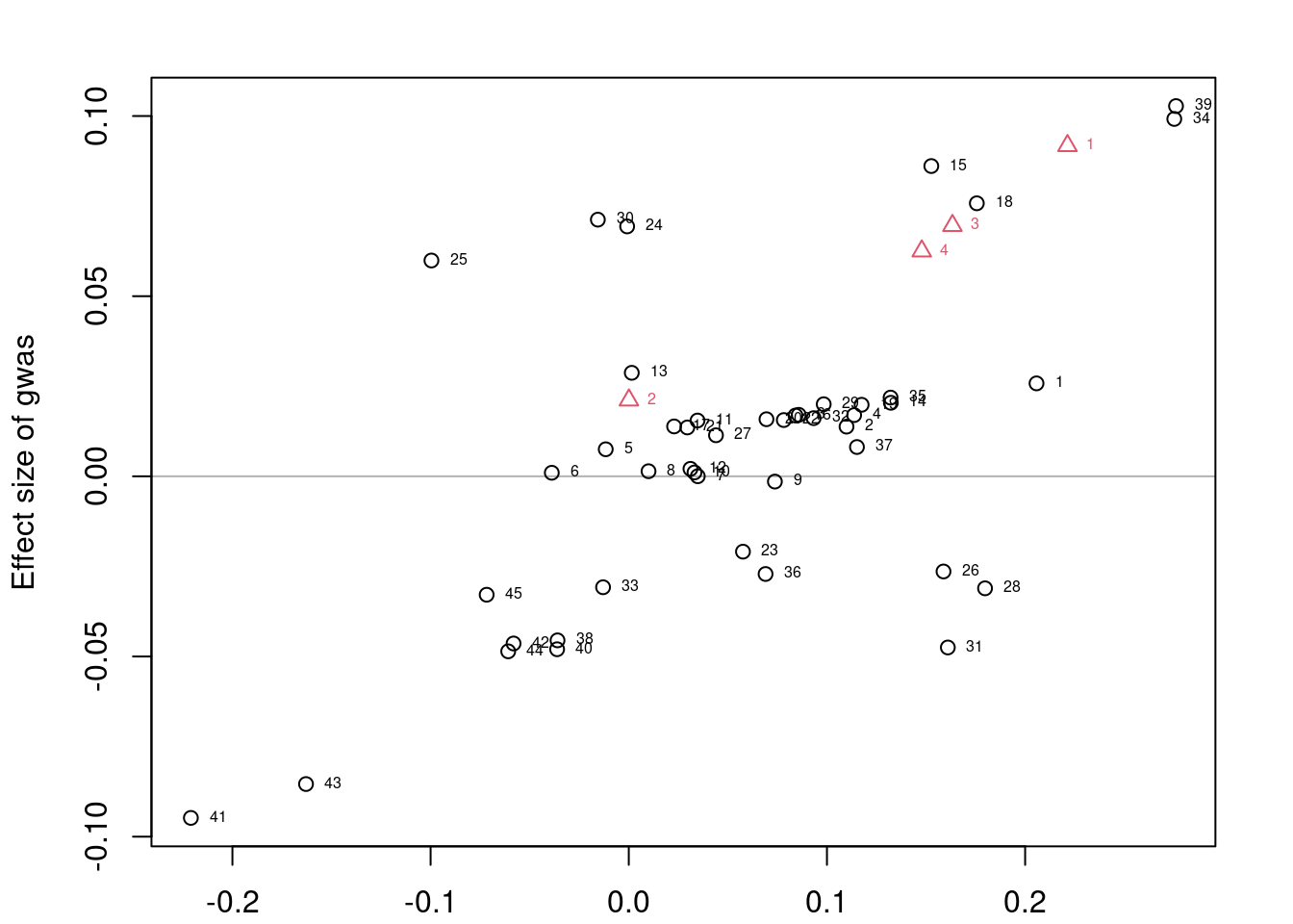

Past versions of unnamed-chunk-8-2.png

Version	Author	Date
d17186e	wesleycrouse	2023-06-08
7f6fbc8	wesleycrouse	2023-05-15
3e493c9	wesleycrouse	2023-05-15

#colocalization
coloc_fit <- list()
nclust <- length(data$beta_hat_a)

options(mc.cores=4)
for (j in 1:nclust) {
  if (length(data$beta_hat_a[[j]])>1){
    coloc_fit[[j]] <- with(data,
                           fitBetaColoc(
                             beta_hat_a = beta_hat_a[[j]],
                             beta_hat_b = beta_hat_b[[j]],
                             se_a = se_a[[j]],
                             se_b = se_b[[j]],
                             Sigma_a = Sigma[[j]],
                             Sigma_b = Sigma[[j]]
                           ))
  } else {
    coloc_fit[[j]] <- list(beta_hat_a=data$beta_hat_a[[j]],
                           beta_hat_b=data$beta_hat_b[[j]])
  }
}

Warning: There were 1355 divergent transitions after warmup. See
https://mc-stan.org/misc/warnings.html#divergent-transitions-after-warmup
to find out why this is a problem and how to eliminate them.

Warning: There were 1086 transitions after warmup that exceeded the maximum treedepth. Increase max_treedepth above 10. See
https://mc-stan.org/misc/warnings.html#maximum-treedepth-exceeded

Warning: There were 2 chains where the estimated Bayesian Fraction of Missing Information was low. See
https://mc-stan.org/misc/warnings.html#bfmi-low

Warning: Examine the pairs() plot to diagnose sampling problems

Warning: The largest R-hat is 1.28, indicating chains have not mixed.
Running the chains for more iterations may help. See
https://mc-stan.org/misc/warnings.html#r-hat

Warning: Bulk Effective Samples Size (ESS) is too low, indicating posterior means and medians may be unreliable.
Running the chains for more iterations may help. See
https://mc-stan.org/misc/warnings.html#bulk-ess

Warning: Tail Effective Samples Size (ESS) is too low, indicating posterior variances and tail quantiles may be unreliable.
Running the chains for more iterations may help. See
https://mc-stan.org/misc/warnings.html#tail-ess

Warning: There were 348 divergent transitions after warmup. See
https://mc-stan.org/misc/warnings.html#divergent-transitions-after-warmup
to find out why this is a problem and how to eliminate them.

Warning: Examine the pairs() plot to diagnose sampling problems

Warning: The largest R-hat is 1.1, indicating chains have not mixed.
Running the chains for more iterations may help. See
https://mc-stan.org/misc/warnings.html#r-hat

Warning: Bulk Effective Samples Size (ESS) is too low, indicating posterior means and medians may be unreliable.
Running the chains for more iterations may help. See
https://mc-stan.org/misc/warnings.html#bulk-ess

Warning: Tail Effective Samples Size (ESS) is too low, indicating posterior variances and tail quantiles may be unreliable.
Running the chains for more iterations may help. See
https://mc-stan.org/misc/warnings.html#tail-ess

res <- list(beta_hat_a = lapply(coloc_fit, `[[`, "beta_hat_a"),
            beta_hat_b = lapply(coloc_fit, `[[`, "beta_hat_b"),
            sd_a = data$se_a,
            sd_b = data$se_b,
            alleles = data$alleles)

res <- extractForSlope(res)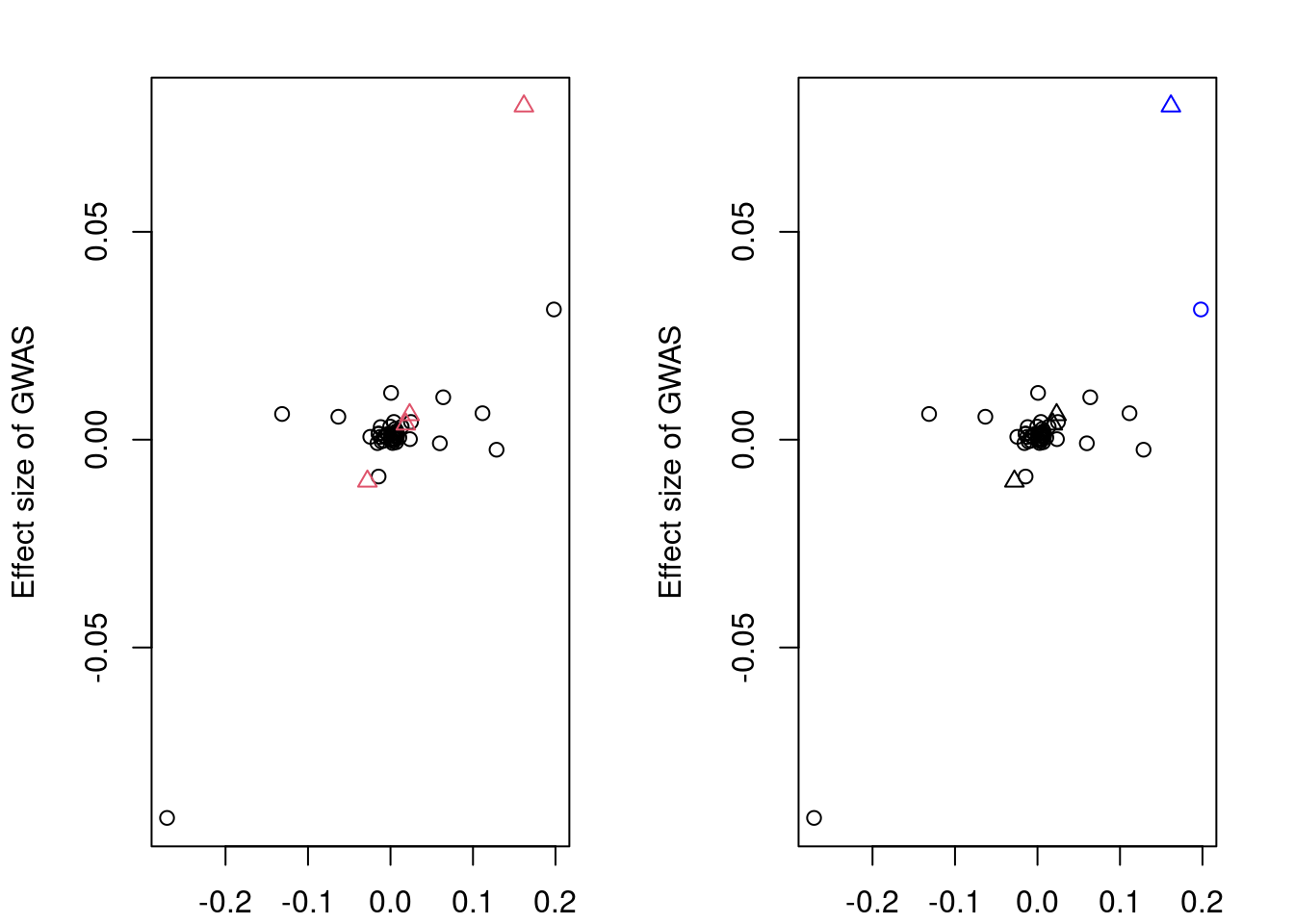

Past versions of unnamed-chunk-8-3.png

Version	Author	Date
d17186e	wesleycrouse	2023-06-08
7f6fbc8	wesleycrouse	2023-05-15
3e493c9	wesleycrouse	2023-05-15

res

$beta_hat_a
[1] 0.1980562 0.1617230

$beta_hat_b
[1] 0.03131939 0.08024581

$sd_a
[1] 0.0846188 0.0596666

$sd_b
[1] 0.01583697 0.01153973

$alleles
          id ref eff
39 rs3800484   T   C
46 rs2439556   A   G

#sort clusters by significance
res$abs_z <- abs(res$beta_hat_a/res$sd_a)
res_sig_order <- order(-res$abs_z)

res$beta_hat_a <- res$beta_hat_a[res_sig_order]
res$beta_hat_b <- res$beta_hat_b[res_sig_order]
res$sd_a <- res$sd_a[res_sig_order]
res$sd_b <- res$sd_b[res_sig_order]
res$alleles <- res$alleles[res_sig_order,,drop=F]
res$abs_z <- NULL

####################

res_bkup <- res

####################

#trim clusters if (absolute) correlation greater than 0.05
if (length(res$alleles$id)>1){
  trim_index <- trimClusters(r2=abs(R_snp[res$alleles$id,res$alleles$id,drop=F]),
                             r2_threshold=0.05)

  if (length(trim_index)>0){
    res$beta_hat_a <- res$beta_hat_a[-trim_index]
    res$beta_hat_b <- res$beta_hat_b[-trim_index]
    res$sd_a <- res$sd_a[-trim_index]
    res$sd_b <- res$sd_b[-trim_index]
    res$alleles <- res$alleles[-trim_index,,drop=F]
  }
}

####################
#visual input data

par(mfrow=c(3,1))

logging::loginfo(gene)

2023-06-12 15:34:01 INFO::ENSG00000215022

par(mar=c(2.1, 4.1, 2.1, 2.1))

plot(df_locus$pos, abs(df_locus$z_gwas), xlab="", ylab="GWAS |Z|")
abline(v=df_locus$pos[df_locus$causal], col="red")

plot(df_locus$pos, abs(df_locus$z_eqtl), xlab="", ylab="eQTL SS |Z|",
     col=colors[df_locus$clump+1])
abline(v=df_locus$pos[df_locus$causal], col="red")

plot(df_locus$pos, abs(df_locus$weight), col="purple", xlab="", ylab="eQTL Lasso |wgt|")
abline(v=df_locus$pos[df_locus$causal], col="red")

breakpoints <- ld_R_info[ld_R_info$index!=c(ld_R_info$index[-1],max(ld_R_info$index)),]
breakpoints <- breakpoints[breakpoints$chrom==chr,]
breakpoints <- breakpoints[breakpoints$pos>min(df_locus$pos) & breakpoints$pos<max(df_locus$pos),]

abline(v=breakpoints$pos)

Past versions of unnamed-chunk-8-4.png

Version	Author	Date
d17186e	wesleycrouse	2023-06-08
7f6fbc8	wesleycrouse	2023-05-15
3e493c9	wesleycrouse	2023-05-15

df_locus$trim <- F
df_locus$trim[match(res_bkup$alleles$id[trim_index], df_locus$id)] <- T
df_locus$color <- colors[df_locus$clump+1]
df_locus[match(res_bkup$alleles$id, df_locus$id),]

               id    z_eqtl chrom      pos    z_gwas causal weight clump  trim
4897517 rs2439556 -3.709932     6 13334307 -7.952074  FALSE      0     2 FALSE
4897409 rs3800484  3.263211     6 13307046  6.488619  FALSE      0     1  TRUE
          color
4897517 #00FFFF
4897409 #FF0000

par(mfrow=c(1,1))

scales::show_col(colors[c(1, res_sig_order+1)])

Past versions of unnamed-chunk-8-5.png

Version	Author	Date
d17186e	wesleycrouse	2023-06-08

####################

if (length(res$beta_hat_a)==1){
  #parametric sample from MRLocus code
  m <- 1e+05
  post_samples <- list(alpha=rnorm(m, res$beta_hat_b, res$sd_b)/rnorm(m, res$beta_hat_a, res$sd_a))
} else {
  #fit MRLocus slope model
  res <- fitSlope(res, iter=10000)
  post_samples <- rstan::extract(res$stanfit)
}

par(mfrow=c(1,1))

#display results
print(res$stanfit, pars=c("alpha","sigma"), probs=c(.1,.9), digits=3)

NULL

if (!is.null(res$stanfit)){
  plotMrlocus(res, main="MRLocus gene-to-trait effect estimate")
} else {
  logging::loginfo("<2 clumps for analysis")
}

2023-06-12 15:34:02 INFO::<2 clumps for analysis

####################
#investigate LD between variants with largest weights and eSNPs for clumps

#variants with largest weight
df_locus <- df_locus[order(-abs(df_locus$weight)),]
df_locus[df_locus$weight!=0,]

               id    z_eqtl chrom      pos    z_gwas causal       weight clump
4897476  rs555100 -3.643406     6 13318609 -8.138288  FALSE  4.85653e-02     1
4897349 rs1550526 -3.317257     6 13295515 -6.491346  FALSE -2.22233e-02     1
4897261 rs9395602  2.626244     6 13278753 -2.367597  FALSE -1.95757e-02     1
4897980 rs2841512 -3.198471     6 13587980 -1.908055  FALSE -1.73881e-02     0
4898103  rs204221 -3.232695     6 13704341 -2.604934  FALSE -7.99743e-03     0
4868316 rs1150609 -2.721145     6 13182501 -1.841752  FALSE  3.94201e-03     0
4897473 rs3823441  3.256555     6 13318030  4.418932  FALSE -3.13081e-03     0
4897262 rs9381884  2.626244     6 13278788 -2.361500  FALSE -5.09785e-05     1
         trim   color
4897476 FALSE #FF0000
4897349 FALSE #FF0000
4897261 FALSE #FF0000
4897980 FALSE   black
4898103 FALSE   black
4868316 FALSE   black
4897473 FALSE   black
4897262 FALSE #FF0000

#eSNPs in the analysis
df_locus[match(res$alleles$id, df_locus$id),]

               id    z_eqtl chrom      pos    z_gwas causal weight clump  trim
4897517 rs2439556 -3.709932     6 13334307 -7.952074  FALSE      0     2 FALSE
          color
4897517 #00FFFF

#LD between confounding SNPs and eSNPs
snplist_all <- c(df_locus$id[df_locus$weight!=0], res$alleles$id)

ld_R_idx <- unique(ld_R_info$index[match(snplist_all, ld_R_info$id)])

R_snp <- lapply(ld_R_files[ld_R_idx], readRDS)

R_snp_info <- lapply(ld_R_info_files[ld_R_idx], fread)
R_snp_info <- lapply(R_snp_info, as.data.frame)

R_snp_index <- lapply(R_snp_info, function(x){x$id %in% snplist_all})

for (j in 1:length(R_snp)){
  R_snp[[j]] <- R_snp[[j]][R_snp_index[[j]],R_snp_index[[j]]]
  R_snp_info[[j]] <- R_snp_info[[j]][R_snp_index[[j]],,drop=F]
}

R_snp_info <- as.data.frame(do.call(rbind, R_snp_info))
R_snp <- as.matrix(Matrix::bdiag(R_snp))

colnames(R_snp) <- R_snp_info$id
rownames(R_snp) <- R_snp_info$id

#number of LD regions
length(ld_R_idx)

[1] 2

#LD between variants
R_snp[snplist_all, snplist_all]

             rs555100   rs1550526    rs9395602    rs2841512    rs204221
rs555100   1.00000000  0.18517096  0.505815561  0.023015009  0.04337648
rs1550526  0.18517096  1.00000000  0.168641522 -0.026414426  0.02045739
rs9395602  0.50581556  0.16864152  1.000000000 -0.008500891 -0.02706590
rs2841512  0.02301501 -0.02641443 -0.008500891  1.000000000  0.77255548
rs204221   0.04337648  0.02045739 -0.027065899  0.772555478  1.00000000
rs1150609  0.00000000  0.00000000  0.000000000  0.000000000  0.00000000
rs3823441 -0.18818972 -0.47797099 -0.029256809  0.049136194  0.01666876
rs9381884  0.50581556  0.16864152  1.000000000 -0.008500891 -0.02706590
rs2439556  0.98146958  0.18700369  0.496965223  0.029135961  0.04911024
          rs1150609   rs3823441    rs9381884   rs2439556
rs555100          0 -0.18818972  0.505815561  0.98146958
rs1550526         0 -0.47797099  0.168641522  0.18700369
rs9395602         0 -0.02925681  1.000000000  0.49696522
rs2841512         0  0.04913619 -0.008500891  0.02913596
rs204221          0  0.01666876 -0.027065899  0.04911024
rs1150609         1  0.00000000  0.000000000  0.00000000
rs3823441         0  1.00000000 -0.029256809 -0.18683534
rs9381884         0 -0.02925681  1.000000000  0.49696522
rs2439556         0 -0.18683534  0.496965223  1.00000000

ENSG00000184898

load("/home/wcrouse/scratch-midway2/mrlocus_image.RData")

####################
#run MR-Locus 

gene <- "ENSG00000184898"

chr <- as.numeric(gtf_df$seqnames[gtf_df$gene_id==gene])

#prepare files for plink
plink_exclude_file <- paste0(temp_dir, "ukb_chr", chr, "_s80.45.2.exclude")

if (!file.exists(plink_exclude_file)){
  #store list of SNPs in .bed file using plink
  system_cmd <- paste0("plink --bfile ",
                       ld_bedfs$file[chr],
                       " --write-snplist --out ",
                       temp_dir, "ukb_chr", chr, "_s80.45.2")
  system(system_cmd)

  #store list of duplicate SNPs in .bed file to exclude
  system_cmd <- paste0("sort ",
                       temp_dir,
                       "ukb_chr", chr, "_s80.45.2.snplist|uniq -d > ",
                       temp_dir,
                       "ukb_chr", chr, "_s80.45.2.exclude")

  system(system_cmd)
}

#clumping using plink
eqtl_current <- eqtl[eqtl$gene_id==gene,]
eqtl_current <- dplyr::rename(eqtl_current, SNP="id", P="pval_nominal")

eqtl_current_file <- paste0(temp_dir, outname_base, ".eqtl_sumstats.", gene, ".temp")
write.table(eqtl_current, file=eqtl_current_file, sep="\t", col.names=T, row.names=F, quote=F)

eqtl_clump_file <- paste0(temp_dir, outname_base, ".eqtl_clumps.", gene, ".temp")
system_cmd <- paste0("plink --bfile ",
                     ld_bedfs$file[chr],
                     " --clump ",
                     eqtl_current_file,
                     " --clump-p1 0.001 --clump-p2 1 --clump-r2 0.1 --clump-kb 500 --out ",
                     eqtl_clump_file,
                     " --exclude ",
                     plink_exclude_file)

#system(system_cmd)
print(system_cmd)

[1] "plink --bfile /home/wcrouse/causalTWAS/simulations/simulation_ctwas_rss_20210416_compare/ukb_chr2_s80.45.2.FUSION2 --clump /home/wcrouse/causalTWAS/simulations/simulation_ctwas_rss_20210416_compare/temp_mrlocus/mrlocus_report_temp.eqtl_sumstats.ENSG00000184898.temp --clump-p1 0.001 --clump-p2 1 --clump-r2 0.1 --clump-kb 500 --out /home/wcrouse/causalTWAS/simulations/simulation_ctwas_rss_20210416_compare/temp_mrlocus/mrlocus_report_temp.eqtl_clumps.ENSG00000184898.temp --exclude /home/wcrouse/causalTWAS/simulations/simulation_ctwas_rss_20210416_compare/temp_mrlocus/ukb_chr2_s80.45.2.exclude"

eqtl_clump_file <- paste0(eqtl_clump_file, ".clumped")

clumps <- read.table(eqtl_clump_file, header=T)
clumps$SP2 <- sapply(1:nrow(clumps), function(x){paste0(clumps$SNP[x], "(1),", clumps$SP2[x])})
clumps <- lapply(clumps$SP2, function(y){unname(sapply(unlist(strsplit(y, ",")), function(x){unlist(strsplit(x, "[(]"))[1]}))})
clumps <- lapply(clumps, function(x){x[x!="NONE"]})

####################

df_locus <- data.frame(id=eqtl_current$SNP, z_eqtl=eqtl_current$slope/eqtl_current$slope_se)
df_locus <- cbind(df_locus, ld_R_info[match(df_locus$id, ld_R_info$id),c("chrom","pos")])
df_locus$z_gwas <- (gwas$Estimate/gwas$Std.Error)[match(df_locus$id, gwas$id)]
df_locus$causal <- df_locus$id %in% names(true_snp_effects) 

weightf_dir <- "/project2/mstephens/causalTWAS/fusion_weights/Adipose_Subcutaneous/"
weightf_gene <- list.files(weightf_dir)
weightf_gene <- paste0(weightf_dir, weightf_gene[grep(gene, weightf_gene)])
load(weightf_gene)

df_locus$weight <- wgt.matrix[match(df_locus$id, rownames(wgt.matrix)),"lasso"]
df_locus$weight[is.na(df_locus$weight)] <- 0

df_locus$clump <- 0

for (j in 1:length(clumps)){
  df_locus$clump[df_locus$id %in% clumps[[j]]] <- j
}

#visualize input data
colors <- c("black", rainbow(length(clumps)))

par(mfrow=c(3,1))

logging::loginfo(gene)

2023-06-12 15:34:44 INFO::ENSG00000184898

par(mar=c(2.1, 4.1, 2.1, 2.1))

plot(df_locus$pos, abs(df_locus$z_gwas), xlab="", ylab="GWAS |Z|")
abline(v=df_locus$pos[df_locus$causal], col="red")

plot(df_locus$pos, abs(df_locus$z_eqtl), xlab="", ylab="eQTL SS |Z|",
     col=colors[df_locus$clump+1])
abline(v=df_locus$pos[df_locus$causal], col="red")

plot(df_locus$pos, abs(df_locus$weight), col="purple", xlab="", ylab="eQTL Lasso |wgt|")
abline(v=df_locus$pos[df_locus$causal], col="red")

breakpoints <- ld_R_info[ld_R_info$index!=c(ld_R_info$index[-1],max(ld_R_info$index)),]
breakpoints <- breakpoints[breakpoints$chrom==chr,]
breakpoints <- breakpoints[breakpoints$pos>min(df_locus$pos) & breakpoints$pos<max(df_locus$pos),]

abline(v=breakpoints$pos)

Past versions of unnamed-chunk-9-1.png

Version	Author	Date
d17186e	wesleycrouse	2023-06-08
7f6fbc8	wesleycrouse	2023-05-15
3e493c9	wesleycrouse	2023-05-15

####################

# #load LD matrix for SNPs in all clumps
# snplist_all <- unlist(clumps)
# 
# ld_R_idx <- unique(ld_R_info$index[match(snplist_all, ld_R_info$id)])
# 
# R_snp <- lapply(ld_R_files[ld_R_idx], readRDS)
# 
# R_snp_info <- lapply(ld_R_info_files[ld_R_idx], fread)
# R_snp_info <- lapply(R_snp_info, as.data.frame)
# 
# R_snp_index <- lapply(R_snp_info, function(x){x$id %in% snplist_all})
# rm(snplist_all)
# 
# for (j in 1:length(R_snp)){
#   R_snp[[j]] <- R_snp[[j]][R_snp_index[[j]],R_snp_index[[j]]]
#   R_snp_info[[j]] <- R_snp_info[[j]][R_snp_index[[j]],,drop=F]
# }
# 
# R_snp_info <- as.data.frame(do.call(rbind, R_snp_info))
# R_snp <- as.matrix(Matrix::bdiag(R_snp))
# 
# colnames(R_snp) <- R_snp_info$id
# rownames(R_snp) <- R_snp_info$id
# 
# 
# 
# R_snp_bkup <- R_snp

####################
#load genotypes and compute LD matrix for SNPs in all clumps
snplist_all <- unlist(clumps)

ld_pvarf <- ld_pvarfs[chr]
ldref_file <- ldref_files[chr]

R_snp_info <- read_pvar(ld_pvarf)
ld_pgen <- prep_pgen(pgenf = ldref_file, ld_pvarf)

sidx <- match(snplist_all, R_snp_info$id)
X.g <- read_pgen(ld_pgen, variantidx = sidx)

R_snp <- Rfast::cora(X.g)
colnames(R_snp) <- snplist_all
rownames(R_snp) <- snplist_all

rm(snplist_all, X.g)

####################

#prepare data object
data <- list(sum_stat=list(),
             ld_mat=list())

for (j in 1:length(clumps)){
  snplist <- clumps[[j]]

  R_snp_current <- R_snp[snplist,snplist,drop=F]
  dimnames(R_snp_current) <- NULL

  R_snp_info_current <- R_snp_info[match(snplist, R_snp_info$id),c("id", "ref", "alt")]

  sumstats_current <- data.frame(id=snplist,
                                 ref=R_snp_info_current$ref,
                                 eff=R_snp_info_current$alt,
                                 beta_hat_eqtl=eqtl_current$slope[match(snplist, eqtl_current$SNP)],
                                 beta_hat_gwas=gwas$Estimate[match(snplist, gwas$id)],
                                 se_eqtl=eqtl_current$slope_se[match(snplist, eqtl_current$SNP)],
                                 se_gwas=gwas$Std.Error[match(snplist, gwas$id)])
  sumstats_current$abs_z <- abs(sumstats_current$beta_hat_eqtl/sumstats_current$se_eqtl)

  data$sum_stat[[j]] <- sumstats_current
  data$ld_mat[[j]] <- R_snp_current
}

par(mfrow=c(1,1))

#collapse high correlation SNP keeping most extreme z score (most significant)
data <- collapseHighCorSNPs(data$sum_stat,
                            data$ld_mat,
                            score="abs_z",
                            plot=F)

pre:  396,164

post: 59,19

data <- flipAllelesAndGather(data$sum_stat,
                             data$ld_mat,
                             snp_id="id",
                             ref="ref",
                             a="eqtl",
                             sep="_",
                             b="gwas",
                             eff="eff",
                             beta="beta_hat",
                             se="se",
                             a2_plink="ref_eqtl",
                             alleles_same=T)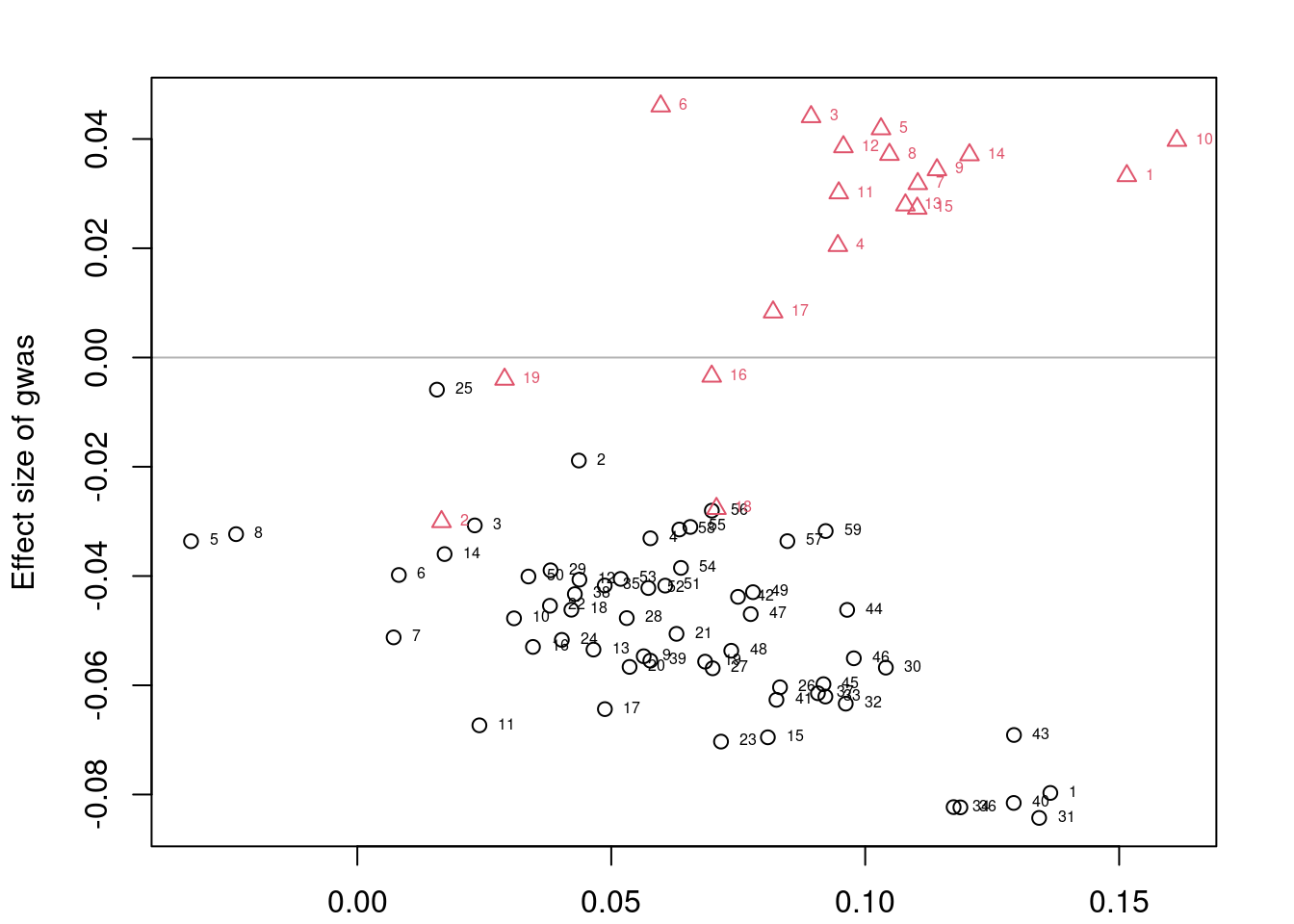

Past versions of unnamed-chunk-9-2.png

Version	Author	Date
d17186e	wesleycrouse	2023-06-08
7f6fbc8	wesleycrouse	2023-05-15
3e493c9	wesleycrouse	2023-05-15

#colocalization
coloc_fit <- list()
nclust <- length(data$beta_hat_a)

options(mc.cores=4)
for (j in 1:nclust) {
  if (length(data$beta_hat_a[[j]])>1){
    coloc_fit[[j]] <- with(data,
                           fitBetaColoc(
                             beta_hat_a = beta_hat_a[[j]],
                             beta_hat_b = beta_hat_b[[j]],
                             se_a = se_a[[j]],
                             se_b = se_b[[j]],
                             Sigma_a = Sigma[[j]],
                             Sigma_b = Sigma[[j]]
                           ))
  } else {
    coloc_fit[[j]] <- list(beta_hat_a=data$beta_hat_a[[j]],
                           beta_hat_b=data$beta_hat_b[[j]])
  }
}

Warning: There were 1013 divergent transitions after warmup. See
https://mc-stan.org/misc/warnings.html#divergent-transitions-after-warmup
to find out why this is a problem and how to eliminate them.

Warning: There were 2307 transitions after warmup that exceeded the maximum treedepth. Increase max_treedepth above 10. See
https://mc-stan.org/misc/warnings.html#maximum-treedepth-exceeded

Warning: There were 4 chains where the estimated Bayesian Fraction of Missing Information was low. See
https://mc-stan.org/misc/warnings.html#bfmi-low

Warning: Examine the pairs() plot to diagnose sampling problems

Warning: The largest R-hat is 1.23, indicating chains have not mixed.
Running the chains for more iterations may help. See
https://mc-stan.org/misc/warnings.html#r-hat

Warning: Bulk Effective Samples Size (ESS) is too low, indicating posterior means and medians may be unreliable.
Running the chains for more iterations may help. See
https://mc-stan.org/misc/warnings.html#bulk-ess

Warning: Tail Effective Samples Size (ESS) is too low, indicating posterior variances and tail quantiles may be unreliable.
Running the chains for more iterations may help. See
https://mc-stan.org/misc/warnings.html#tail-ess

Warning: There were 1254 divergent transitions after warmup. See
https://mc-stan.org/misc/warnings.html#divergent-transitions-after-warmup
to find out why this is a problem and how to eliminate them.

Warning: There were 95 transitions after warmup that exceeded the maximum treedepth. Increase max_treedepth above 10. See
https://mc-stan.org/misc/warnings.html#maximum-treedepth-exceeded

Warning: There were 2 chains where the estimated Bayesian Fraction of Missing Information was low. See
https://mc-stan.org/misc/warnings.html#bfmi-low

Warning: Examine the pairs() plot to diagnose sampling problems

Warning: The largest R-hat is 1.36, indicating chains have not mixed.
Running the chains for more iterations may help. See
https://mc-stan.org/misc/warnings.html#r-hat

Warning: Bulk Effective Samples Size (ESS) is too low, indicating posterior means and medians may be unreliable.
Running the chains for more iterations may help. See
https://mc-stan.org/misc/warnings.html#bulk-ess

Warning: Tail Effective Samples Size (ESS) is too low, indicating posterior variances and tail quantiles may be unreliable.
Running the chains for more iterations may help. See
https://mc-stan.org/misc/warnings.html#tail-ess

res <- list(beta_hat_a = lapply(coloc_fit, `[[`, "beta_hat_a"),
            beta_hat_b = lapply(coloc_fit, `[[`, "beta_hat_b"),
            sd_a = data$se_a,
            sd_b = data$se_b,
            alleles = data$alleles)

res <- extractForSlope(res)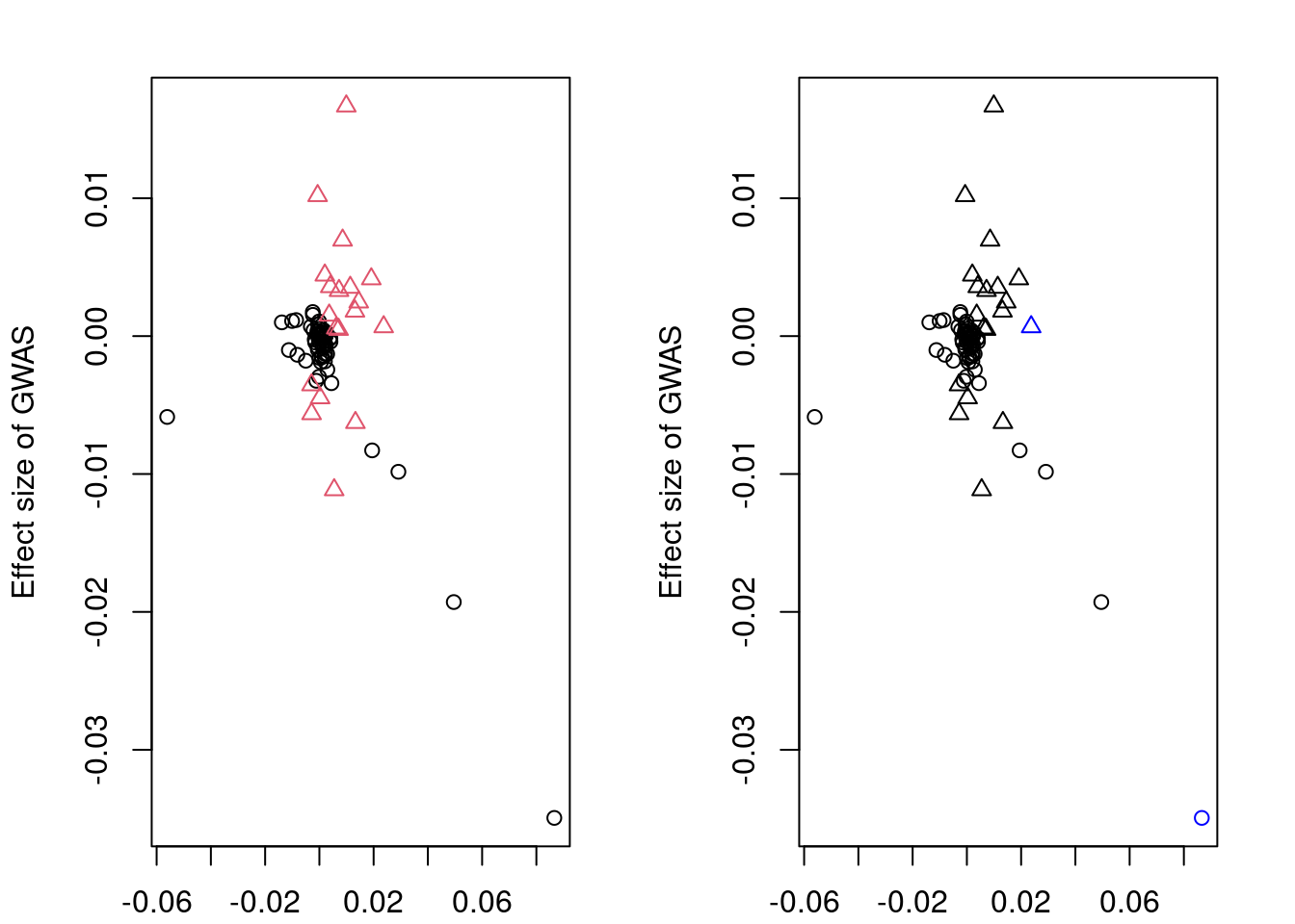

Past versions of unnamed-chunk-9-3.png

Version	Author	Date
d17186e	wesleycrouse	2023-06-08
7f6fbc8	wesleycrouse	2023-05-15
3e493c9	wesleycrouse	2023-05-15

res

$beta_hat_a
[1] 0.08661205 0.02370354

$beta_hat_b
[1] -0.0349405113  0.0006716198

$sd_a
[1] 0.0282915 0.0413816

$sd_b
[1] 0.009899139 0.017600476

$alleles
          id ref eff
31   rs11730   G   A
60 rs9677576   A   G

#sort clusters by significance
res$abs_z <- abs(res$beta_hat_a/res$sd_a)
res_sig_order <- order(-res$abs_z)

res$beta_hat_a <- res$beta_hat_a[res_sig_order]
res$beta_hat_b <- res$beta_hat_b[res_sig_order]
res$sd_a <- res$sd_a[res_sig_order]
res$sd_b <- res$sd_b[res_sig_order]
res$alleles <- res$alleles[res_sig_order,,drop=F]
res$abs_z <- NULL

####################

res_bkup <- res

####################

#trim clusters if (absolute) correlation greater than 0.05
if (length(res$alleles$id)>1){
  trim_index <- trimClusters(r2=abs(R_snp[res$alleles$id,res$alleles$id,drop=F]),
                             r2_threshold=0.05)

  if (length(trim_index)>0){
    res$beta_hat_a <- res$beta_hat_a[-trim_index]
    res$beta_hat_b <- res$beta_hat_b[-trim_index]
    res$sd_a <- res$sd_a[-trim_index]
    res$sd_b <- res$sd_b[-trim_index]
    res$alleles <- res$alleles[-trim_index,,drop=F]
  }
}

####################
#visual input data

par(mfrow=c(3,1))

logging::loginfo(gene)

2023-06-12 15:36:29 INFO::ENSG00000184898

par(mar=c(2.1, 4.1, 2.1, 2.1))

plot(df_locus$pos, abs(df_locus$z_gwas), xlab="", ylab="GWAS |Z|")
abline(v=df_locus$pos[df_locus$causal], col="red")

plot(df_locus$pos, abs(df_locus$z_eqtl), xlab="", ylab="eQTL SS |Z|",
     col=colors[df_locus$clump+1])
abline(v=df_locus$pos[df_locus$causal], col="red")

plot(df_locus$pos, abs(df_locus$weight), col="purple", xlab="", ylab="eQTL Lasso |wgt|")
abline(v=df_locus$pos[df_locus$causal], col="red")

breakpoints <- ld_R_info[ld_R_info$index!=c(ld_R_info$index[-1],max(ld_R_info$index)),]
breakpoints <- breakpoints[breakpoints$chrom==chr,]
breakpoints <- breakpoints[breakpoints$pos>min(df_locus$pos) & breakpoints$pos<max(df_locus$pos),]

abline(v=breakpoints$pos)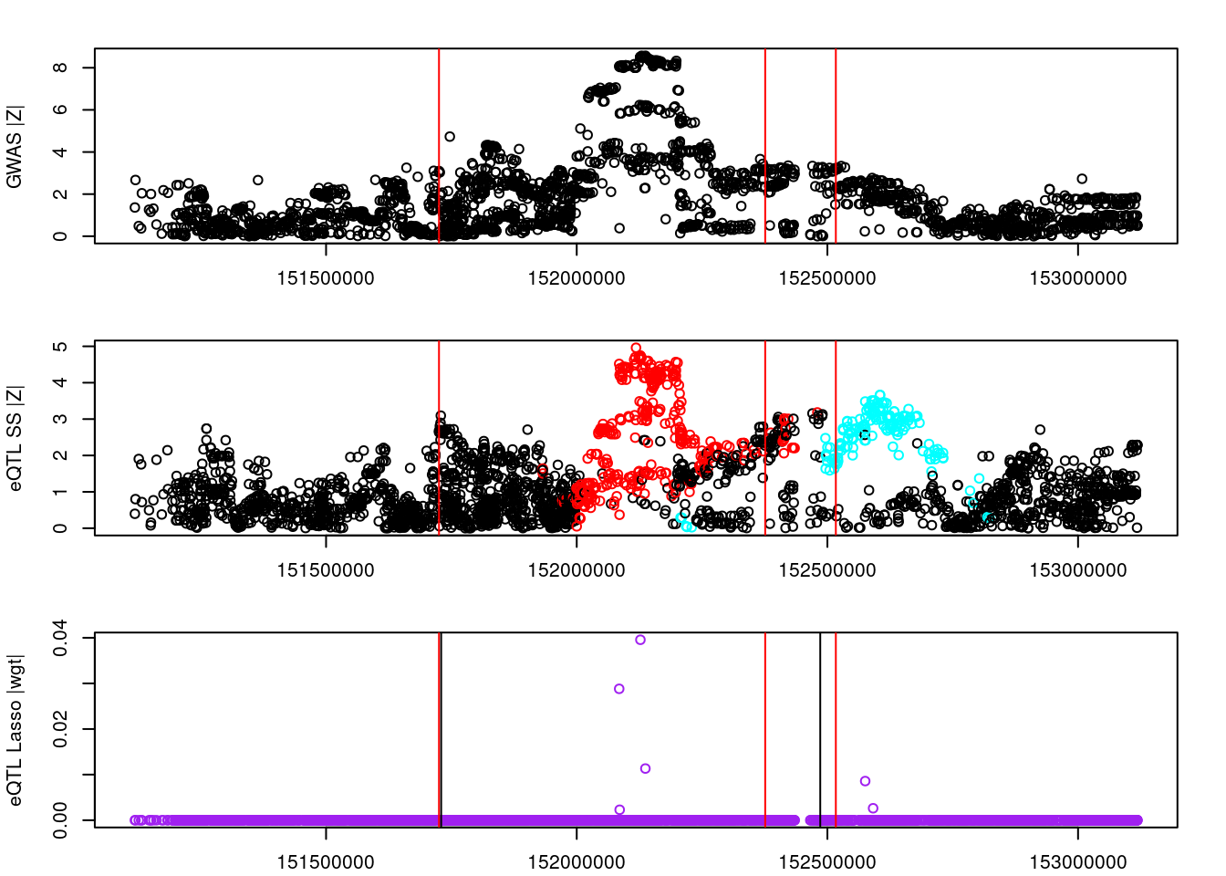

Past versions of unnamed-chunk-9-4.png

Version	Author	Date
d17186e	wesleycrouse	2023-06-08
7f6fbc8	wesleycrouse	2023-05-15
3e493c9	wesleycrouse	2023-05-15

df_locus$trim <- F
df_locus$trim[match(res_bkup$alleles$id[trim_index], df_locus$id)] <- T
df_locus$color <- colors[df_locus$clump+1]
df_locus[match(res_bkup$alleles$id, df_locus$id),]

               id   z_eqtl chrom       pos    z_gwas causal     weight clump
2813724   rs11730 4.745171     2 152127011 -8.513674  FALSE -0.0395602     1
2814517 rs9677576 3.661217     2 152604697  1.890673  FALSE  0.0000000     2
         trim   color
2813724 FALSE #FF0000
2814517  TRUE #00FFFF

par(mfrow=c(1,1))

scales::show_col(colors[c(1, res_sig_order+1)])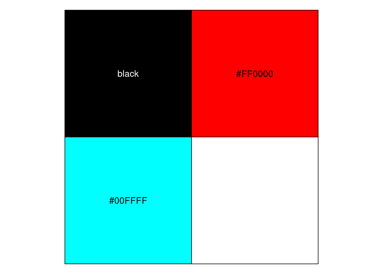

Past versions of unnamed-chunk-9-5.png

Version	Author	Date
d17186e	wesleycrouse	2023-06-08

####################

if (length(res$beta_hat_a)==1){
  #parametric sample from MRLocus code
  m <- 1e+05
  post_samples <- list(alpha=rnorm(m, res$beta_hat_b, res$sd_b)/rnorm(m, res$beta_hat_a, res$sd_a))
} else {
  #fit MRLocus slope model
  res <- fitSlope(res, iter=10000)
  post_samples <- rstan::extract(res$stanfit)
}

par(mfrow=c(1,1))

#display results
print(res$stanfit, pars=c("alpha","sigma"), probs=c(.1,.9), digits=3)

NULL

if (!is.null(res$stanfit)){
  plotMrlocus(res, main="MRLocus gene-to-trait effect estimate")
} else {
  logging::loginfo("<2 clumps for analysis")
}

2023-06-12 15:36:30 INFO::<2 clumps for analysis

####################
#investigate LD between variants with largest weights and eSNPs for clumps

#variants with largest weight
df_locus <- df_locus[order(-abs(df_locus$weight)),]
df_locus[df_locus$weight!=0,]

                id    z_eqtl chrom       pos    z_gwas causal       weight
2813724    rs11730  4.745171     2 152127011 -8.513674  FALSE -3.95602e-02
2813649   rs289903 -4.515707     2 152084705  8.062208  FALSE -2.88088e-02
2813751  rs3856557  4.435029     2 152136961 -8.485281  FALSE -1.13303e-02
2814465  rs4664498  3.482618     2 152575417  1.839083  FALSE  8.57801e-03
2814492 rs11896217  3.508597     2 152591189  2.124467  FALSE  2.62155e-03
2813651   rs289904 -4.224670     2 152085643  8.087215  FALSE -2.29195e-03
2814497  rs4393745  3.508597     2 152594206  2.154522  FALSE  6.82696e-06
        clump  trim   color
2813724     1 FALSE #FF0000
2813649     1 FALSE #FF0000
2813751     1 FALSE #FF0000
2814465     2 FALSE #00FFFF
2814492     2 FALSE #00FFFF
2813651     1 FALSE #FF0000
2814497     2 FALSE #00FFFF

#eSNPs in the analysis
df_locus[match(res$alleles$id, df_locus$id),]

             id   z_eqtl chrom       pos    z_gwas causal     weight clump
2813724 rs11730 4.745171     2 152127011 -8.513674  FALSE -0.0395602     1
         trim   color
2813724 FALSE #FF0000

#LD between confounding SNPs and eSNPs
snplist_all <- c(df_locus$id[df_locus$weight!=0], res$alleles$id)

ld_R_idx <- unique(ld_R_info$index[match(snplist_all, ld_R_info$id)])

R_snp <- lapply(ld_R_files[ld_R_idx], readRDS)

R_snp_info <- lapply(ld_R_info_files[ld_R_idx], fread)
R_snp_info <- lapply(R_snp_info, as.data.frame)

R_snp_index <- lapply(R_snp_info, function(x){x$id %in% snplist_all})

for (j in 1:length(R_snp)){
  R_snp[[j]] <- R_snp[[j]][R_snp_index[[j]],R_snp_index[[j]]]
  R_snp_info[[j]] <- R_snp_info[[j]][R_snp_index[[j]],,drop=F]
}

R_snp_info <- as.data.frame(do.call(rbind, R_snp_info))
R_snp <- as.matrix(Matrix::bdiag(R_snp))

colnames(R_snp) <- R_snp_info$id
rownames(R_snp) <- R_snp_info$id

#number of LD regions
length(ld_R_idx)

[1] 2

#LD between variants
R_snp[snplist_all, snplist_all]

              rs11730   rs289903  rs3856557 rs4664498 rs11896217   rs289904
rs11730     1.0000000 -0.9055700  0.9992733 0.0000000  0.0000000 -0.9050076
rs289903   -0.9055700  1.0000000 -0.9042423 0.0000000  0.0000000  0.9988528
rs3856557   0.9992733 -0.9042423  1.0000000 0.0000000  0.0000000 -0.9036801
rs4664498   0.0000000  0.0000000  0.0000000 1.0000000  0.8924160  0.0000000
rs11896217  0.0000000  0.0000000  0.0000000 0.8924160  1.0000000  0.0000000
rs289904   -0.9050076  0.9988528 -0.9036801 0.0000000  0.0000000  1.0000000
rs4393745   0.0000000  0.0000000  0.0000000 0.8919337  0.9999043  0.0000000
rs11730     1.0000000 -0.9055700  0.9992733 0.0000000  0.0000000 -0.9050076
           rs4393745    rs11730
rs11730    0.0000000  1.0000000
rs289903   0.0000000 -0.9055700
rs3856557  0.0000000  0.9992733
rs4664498  0.8919337  0.0000000
rs11896217 0.9999043  0.0000000
rs289904   0.0000000 -0.9050076
rs4393745  1.0000000  0.0000000
rs11730    0.0000000  1.0000000

False positives

ENSG00000243335

set.seed(13450)

load("/home/wcrouse/scratch-midway2/mrlocus_image.RData")

####################
#run MR-Locus 

gene <- "ENSG00000243335"

chr <- as.numeric(gtf_df$seqnames[gtf_df$gene_id==gene])

#prepare files for plink
plink_exclude_file <- paste0(temp_dir, "ukb_chr", chr, "_s80.45.2.exclude")

if (!file.exists(plink_exclude_file)){
  #store list of SNPs in .bed file using plink
  system_cmd <- paste0("plink --bfile ",
                       ld_bedfs$file[chr],
                       " --write-snplist --out ",
                       temp_dir, "ukb_chr", chr, "_s80.45.2")
  system(system_cmd)

  #store list of duplicate SNPs in .bed file to exclude
  system_cmd <- paste0("sort ",
                       temp_dir,
                       "ukb_chr", chr, "_s80.45.2.snplist|uniq -d > ",
                       temp_dir,
                       "ukb_chr", chr, "_s80.45.2.exclude")

  system(system_cmd)
}

#clumping using plink
eqtl_current <- eqtl[eqtl$gene_id==gene,]
eqtl_current <- dplyr::rename(eqtl_current, SNP="id", P="pval_nominal")

eqtl_current_file <- paste0(temp_dir, outname_base, ".eqtl_sumstats.", gene, ".temp")
write.table(eqtl_current, file=eqtl_current_file, sep="\t", col.names=T, row.names=F, quote=F)

eqtl_clump_file <- paste0(temp_dir, outname_base, ".eqtl_clumps.", gene, ".temp")
system_cmd <- paste0("plink --bfile ",
                     ld_bedfs$file[chr],
                     " --clump ",
                     eqtl_current_file,
                     " --clump-p1 0.001 --clump-p2 1 --clump-r2 0.1 --clump-kb 500 --out ",
                     eqtl_clump_file,
                     " --exclude ",
                     plink_exclude_file)

#system(system_cmd)
print(system_cmd)

[1] "plink --bfile /home/wcrouse/causalTWAS/simulations/simulation_ctwas_rss_20210416_compare/ukb_chr7_s80.45.2.FUSION7 --clump /home/wcrouse/causalTWAS/simulations/simulation_ctwas_rss_20210416_compare/temp_mrlocus/mrlocus_report_temp.eqtl_sumstats.ENSG00000243335.temp --clump-p1 0.001 --clump-p2 1 --clump-r2 0.1 --clump-kb 500 --out /home/wcrouse/causalTWAS/simulations/simulation_ctwas_rss_20210416_compare/temp_mrlocus/mrlocus_report_temp.eqtl_clumps.ENSG00000243335.temp --exclude /home/wcrouse/causalTWAS/simulations/simulation_ctwas_rss_20210416_compare/temp_mrlocus/ukb_chr7_s80.45.2.exclude"

eqtl_clump_file <- paste0(eqtl_clump_file, ".clumped")

clumps <- read.table(eqtl_clump_file, header=T)
clumps$SP2 <- sapply(1:nrow(clumps), function(x){paste0(clumps$SNP[x], "(1),", clumps$SP2[x])})
clumps <- lapply(clumps$SP2, function(y){unname(sapply(unlist(strsplit(y, ",")), function(x){unlist(strsplit(x, "[(]"))[1]}))})
clumps <- lapply(clumps, function(x){x[x!="NONE"]})

####################

df_locus <- data.frame(id=eqtl_current$SNP, z_eqtl=eqtl_current$slope/eqtl_current$slope_se)
df_locus <- cbind(df_locus, ld_R_info[match(df_locus$id, ld_R_info$id),c("chrom","pos")])
df_locus$z_gwas <- (gwas$Estimate/gwas$Std.Error)[match(df_locus$id, gwas$id)]
df_locus$causal <- df_locus$id %in% names(true_snp_effects) 

weightf_dir <- "/project2/mstephens/causalTWAS/fusion_weights/Adipose_Subcutaneous/"
weightf_gene <- list.files(weightf_dir)
weightf_gene <- paste0(weightf_dir, weightf_gene[grep(gene, weightf_gene)])
load(weightf_gene)

df_locus$weight <- wgt.matrix[match(df_locus$id, rownames(wgt.matrix)),"lasso"]
df_locus$weight[is.na(df_locus$weight)] <- 0

df_locus$clump <- 0

for (j in 1:length(clumps)){
  df_locus$clump[df_locus$id %in% clumps[[j]]] <- j
}

#visualize input data
colors <- c("black", rainbow(length(clumps)))

par(mfrow=c(3,1))

logging::loginfo(gene)

2023-06-12 15:37:13 INFO::ENSG00000243335

par(mar=c(2.1, 4.1, 2.1, 2.1))

plot(df_locus$pos, abs(df_locus$z_gwas), xlab="", ylab="GWAS |Z|")
abline(v=df_locus$pos[df_locus$causal], col="red")

plot(df_locus$pos, abs(df_locus$z_eqtl), xlab="", ylab="eQTL SS |Z|",
     col=colors[df_locus$clump+1])
abline(v=df_locus$pos[df_locus$causal], col="red")

plot(df_locus$pos, abs(df_locus$weight), col="purple", xlab="", ylab="eQTL Lasso |wgt|")
abline(v=df_locus$pos[df_locus$causal], col="red")

breakpoints <- ld_R_info[ld_R_info$index!=c(ld_R_info$index[-1],max(ld_R_info$index)),]
breakpoints <- breakpoints[breakpoints$chrom==chr,]
breakpoints <- breakpoints[breakpoints$pos>min(df_locus$pos) & breakpoints$pos<max(df_locus$pos),]

abline(v=breakpoints$pos)

Past versions of unnamed-chunk-10-1.png

Version	Author	Date
d17186e	wesleycrouse	2023-06-08

####################

# #load LD matrix for SNPs in all clumps
# snplist_all <- unlist(clumps)
# 
# ld_R_idx <- unique(ld_R_info$index[match(snplist_all, ld_R_info$id)])
# 
# R_snp <- lapply(ld_R_files[ld_R_idx], readRDS)
# 
# R_snp_info <- lapply(ld_R_info_files[ld_R_idx], fread)
# R_snp_info <- lapply(R_snp_info, as.data.frame)
# 
# R_snp_index <- lapply(R_snp_info, function(x){x$id %in% snplist_all})
# rm(snplist_all)
# 
# for (j in 1:length(R_snp)){
#   R_snp[[j]] <- R_snp[[j]][R_snp_index[[j]],R_snp_index[[j]]]
#   R_snp_info[[j]] <- R_snp_info[[j]][R_snp_index[[j]],,drop=F]
# }
# 
# R_snp_info <- as.data.frame(do.call(rbind, R_snp_info))
# R_snp <- as.matrix(Matrix::bdiag(R_snp))
# 
# colnames(R_snp) <- R_snp_info$id
# rownames(R_snp) <- R_snp_info$id
# 
# 
# 
# R_snp_bkup <- R_snp

####################
#load genotypes and compute LD matrix for SNPs in all clumps
snplist_all <- unlist(clumps)

ld_pvarf <- ld_pvarfs[chr]
ldref_file <- ldref_files[chr]

R_snp_info <- read_pvar(ld_pvarf)
ld_pgen <- prep_pgen(pgenf = ldref_file, ld_pvarf)

sidx <- match(snplist_all, R_snp_info$id)
X.g <- read_pgen(ld_pgen, variantidx = sidx)

R_snp <- Rfast::cora(X.g)
colnames(R_snp) <- snplist_all
rownames(R_snp) <- snplist_all

rm(snplist_all, X.g)

####################

#prepare data object
data <- list(sum_stat=list(),
             ld_mat=list())

for (j in 1:length(clumps)){
  snplist <- clumps[[j]]

  R_snp_current <- R_snp[snplist,snplist,drop=F]
  dimnames(R_snp_current) <- NULL

  R_snp_info_current <- R_snp_info[match(snplist, R_snp_info$id),c("id", "ref", "alt")]

  sumstats_current <- data.frame(id=snplist,
                                 ref=R_snp_info_current$ref,
                                 eff=R_snp_info_current$alt,
                                 beta_hat_eqtl=eqtl_current$slope[match(snplist, eqtl_current$SNP)],
                                 beta_hat_gwas=gwas$Estimate[match(snplist, gwas$id)],
                                 se_eqtl=eqtl_current$slope_se[match(snplist, eqtl_current$SNP)],
                                 se_gwas=gwas$Std.Error[match(snplist, gwas$id)])
  sumstats_current$abs_z <- abs(sumstats_current$beta_hat_eqtl/sumstats_current$se_eqtl)

  data$sum_stat[[j]] <- sumstats_current
  data$ld_mat[[j]] <- R_snp_current
}

par(mfrow=c(1,1))

#collapse high correlation SNP keeping most extreme z score (most significant)
data <- collapseHighCorSNPs(data$sum_stat,
                            data$ld_mat,
                            score="abs_z",
                            plot=F)

pre:  541,338

post: 37,28

data <- flipAllelesAndGather(data$sum_stat,
                             data$ld_mat,
                             snp_id="id",
                             ref="ref",
                             a="eqtl",
                             sep="_",
                             b="gwas",
                             eff="eff",
                             beta="beta_hat",
                             se="se",
                             a2_plink="ref_eqtl",
                             alleles_same=T)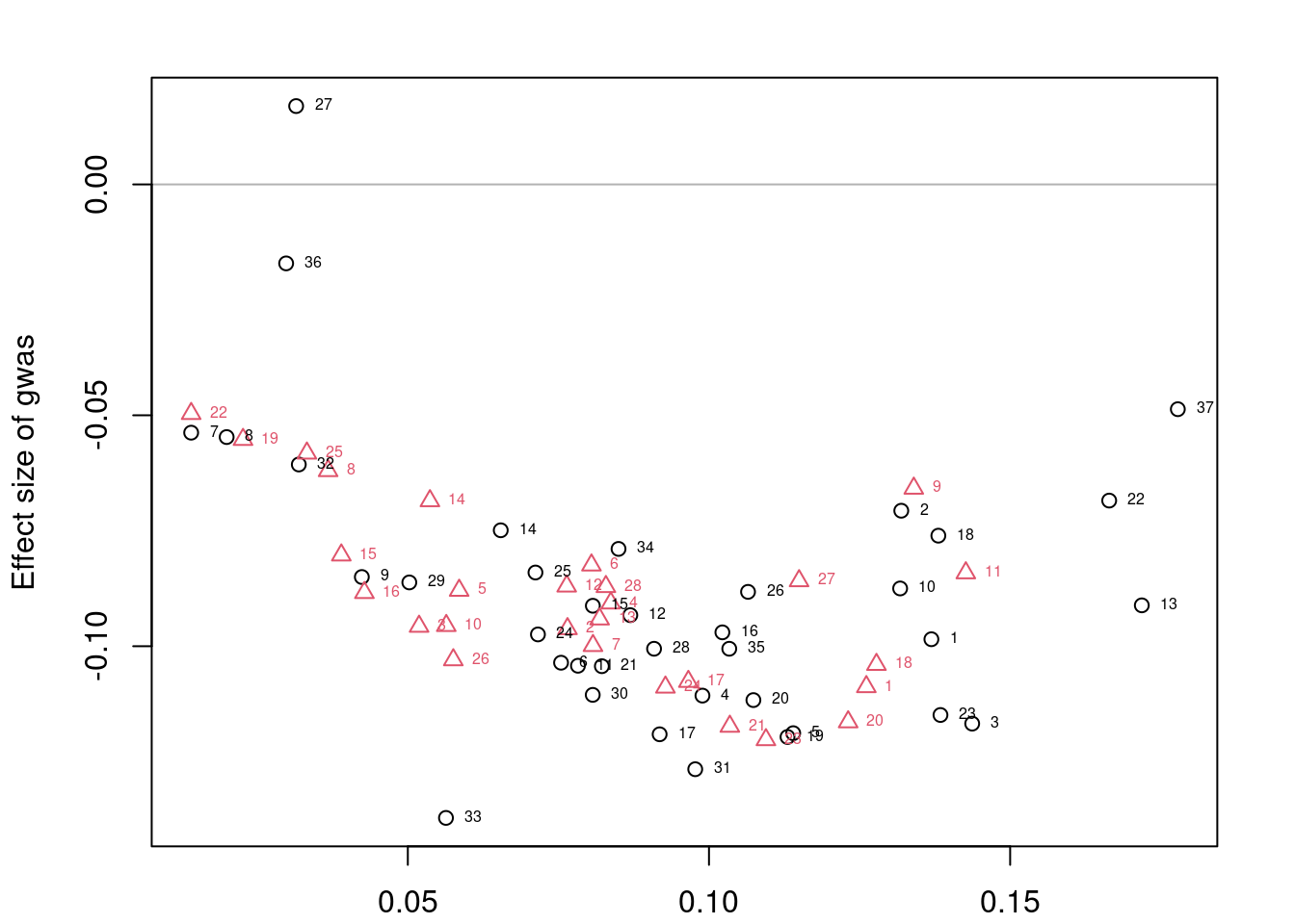

Past versions of unnamed-chunk-10-2.png

Version	Author	Date
d17186e	wesleycrouse	2023-06-08

#colocalization
coloc_fit <- list()
nclust <- length(data$beta_hat_a)

options(mc.cores=4)
for (j in 1:nclust) {
  if (length(data$beta_hat_a[[j]])>1){
    coloc_fit[[j]] <- with(data,
                           fitBetaColoc(
                             beta_hat_a = beta_hat_a[[j]],
                             beta_hat_b = beta_hat_b[[j]],
                             se_a = se_a[[j]],
                             se_b = se_b[[j]],
                             Sigma_a = Sigma[[j]],
                             Sigma_b = Sigma[[j]]
                           ))
  } else {
    coloc_fit[[j]] <- list(beta_hat_a=data$beta_hat_a[[j]],
                           beta_hat_b=data$beta_hat_b[[j]])
  }
}

Warning: There were 1153 divergent transitions after warmup. See
https://mc-stan.org/misc/warnings.html#divergent-transitions-after-warmup
to find out why this is a problem and how to eliminate them.

Warning: There were 225 transitions after warmup that exceeded the maximum treedepth. Increase max_treedepth above 10. See
https://mc-stan.org/misc/warnings.html#maximum-treedepth-exceeded

Warning: There were 2 chains where the estimated Bayesian Fraction of Missing Information was low. See
https://mc-stan.org/misc/warnings.html#bfmi-low

Warning: Examine the pairs() plot to diagnose sampling problems

Warning: The largest R-hat is 1.2, indicating chains have not mixed.
Running the chains for more iterations may help. See
https://mc-stan.org/misc/warnings.html#r-hat

Warning: Bulk Effective Samples Size (ESS) is too low, indicating posterior means and medians may be unreliable.
Running the chains for more iterations may help. See
https://mc-stan.org/misc/warnings.html#bulk-ess

Warning: Tail Effective Samples Size (ESS) is too low, indicating posterior variances and tail quantiles may be unreliable.
Running the chains for more iterations may help. See
https://mc-stan.org/misc/warnings.html#tail-ess

Warning: There were 658 divergent transitions after warmup. See
https://mc-stan.org/misc/warnings.html#divergent-transitions-after-warmup
to find out why this is a problem and how to eliminate them.

Warning: There were 236 transitions after warmup that exceeded the maximum treedepth. Increase max_treedepth above 10. See
https://mc-stan.org/misc/warnings.html#maximum-treedepth-exceeded

Warning: There were 3 chains where the estimated Bayesian Fraction of Missing Information was low. See
https://mc-stan.org/misc/warnings.html#bfmi-low

Warning: Examine the pairs() plot to diagnose sampling problems

Warning: Bulk Effective Samples Size (ESS) is too low, indicating posterior means and medians may be unreliable.
Running the chains for more iterations may help. See
https://mc-stan.org/misc/warnings.html#bulk-ess

Warning: Tail Effective Samples Size (ESS) is too low, indicating posterior variances and tail quantiles may be unreliable.
Running the chains for more iterations may help. See
https://mc-stan.org/misc/warnings.html#tail-ess

res <- list(beta_hat_a = lapply(coloc_fit, `[[`, "beta_hat_a"),
            beta_hat_b = lapply(coloc_fit, `[[`, "beta_hat_b"),
            sd_a = data$se_a,
            sd_b = data$se_b,
            alleles = data$alleles)

res <- extractForSlope(res)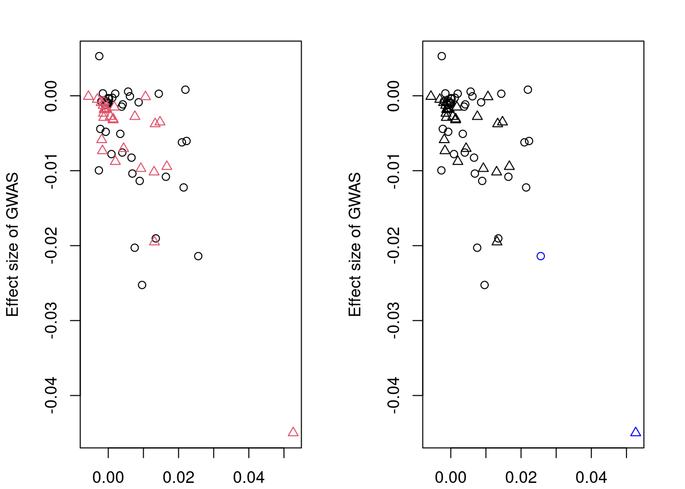

Past versions of unnamed-chunk-10-3.png

Version	Author	Date
d17186e	wesleycrouse	2023-06-08

res

$beta_hat_a
[1] 0.02560447 0.05262674

$beta_hat_b
[1] -0.02139649 -0.04498408

$sd_a
[1] 0.0339436 0.0303630

$sd_b
[1] 0.01124993 0.01070247

$alleles
           id ref eff
3  rs28817617   G   A
60   rs313829   G   A

#sort clusters by significance
res$abs_z <- abs(res$beta_hat_a/res$sd_a)
res_sig_order <- order(-res$abs_z)

res$beta_hat_a <- res$beta_hat_a[res_sig_order]
res$beta_hat_b <- res$beta_hat_b[res_sig_order]
res$sd_a <- res$sd_a[res_sig_order]
res$sd_b <- res$sd_b[res_sig_order]
res$alleles <- res$alleles[res_sig_order,,drop=F]
res$abs_z <- NULL

####################

res_bkup <- res

####################

#trim clusters if (absolute) correlation greater than 0.05
if (length(res$alleles$id)>1){
  trim_index <- trimClusters(r2=abs(R_snp[res$alleles$id,res$alleles$id,drop=F]),
                             r2_threshold=0.05)

  if (length(trim_index)>0){
    res$beta_hat_a <- res$beta_hat_a[-trim_index]
    res$beta_hat_b <- res$beta_hat_b[-trim_index]
    res$sd_a <- res$sd_a[-trim_index]
    res$sd_b <- res$sd_b[-trim_index]
    res$alleles <- res$alleles[-trim_index,,drop=F]
  }
}

####################
#visual input data

par(mfrow=c(3,1))

logging::loginfo(gene)

2023-06-12 15:38:13 INFO::ENSG00000243335

par(mar=c(2.1, 4.1, 2.1, 2.1))

plot(df_locus$pos, abs(df_locus$z_gwas), xlab="", ylab="GWAS |Z|")
abline(v=df_locus$pos[df_locus$causal], col="red")

plot(df_locus$pos, abs(df_locus$z_eqtl), xlab="", ylab="eQTL SS |Z|",
     col=colors[df_locus$clump+1])
abline(v=df_locus$pos[df_locus$causal], col="red")

plot(df_locus$pos, abs(df_locus$weight), col="purple", xlab="", ylab="eQTL Lasso |wgt|")
abline(v=df_locus$pos[df_locus$causal], col="red")

breakpoints <- ld_R_info[ld_R_info$index!=c(ld_R_info$index[-1],max(ld_R_info$index)),]
breakpoints <- breakpoints[breakpoints$chrom==chr,]
breakpoints <- breakpoints[breakpoints$pos>min(df_locus$pos) & breakpoints$pos<max(df_locus$pos),]

abline(v=breakpoints$pos)

Past versions of unnamed-chunk-10-4.png

Version	Author	Date
d17186e	wesleycrouse	2023-06-08

df_locus$trim <- F
df_locus$trim[match(res_bkup$alleles$id[trim_index], df_locus$id)] <- T
df_locus$color <- colors[df_locus$clump+1]
df_locus[match(res_bkup$alleles$id, df_locus$id),]

                id   z_eqtl chrom      pos    z_gwas causal weight clump  trim
5526879   rs313829 3.604848     7 65552497 -11.23665  FALSE      0     2 FALSE
5527815 rs28817617 4.233434     7 66077355 -10.37869  FALSE      0     1  TRUE
          color
5526879 #00FFFF
5527815 #FF0000

par(mfrow=c(1,1))

scales::show_col(colors[c(1, res_sig_order+1)])

Past versions of unnamed-chunk-10-5.png

Version	Author	Date
d17186e	wesleycrouse	2023-06-08

####################

if (length(res$beta_hat_a)==1){
  #parametric sample from MRLocus code
  m <- 1e+05
  post_samples <- list(alpha=rnorm(m, res$beta_hat_b, res$sd_b)/rnorm(m, res$beta_hat_a, res$sd_a))
} else {
  #fit MRLocus slope model
  res <- fitSlope(res, iter=10000)
  post_samples <- rstan::extract(res$stanfit)
}

par(mfrow=c(1,1))

#display results
print(res$stanfit, pars=c("alpha","sigma"), probs=c(.1,.9), digits=3)

NULL

if (!is.null(res$stanfit)){
  plotMrlocus(res, main="MRLocus gene-to-trait effect estimate")
} else {
  logging::loginfo("<2 clumps for analysis")
}

2023-06-12 15:38:14 INFO::<2 clumps for analysis

####################
#investigate LD between confounding variants and eSNPs for clumps

#confounding causal SNPs
df_locus[df_locus$causal,]

              id    z_eqtl chrom      pos   z_gwas causal weight clump  trim
5527360 rs778685 -3.392917     7 65836176 11.90402   TRUE      0     1 FALSE
          color
5527360 #FF0000

#eSNPs in the analysis
df_locus[match(res$alleles$id, df_locus$id),]

              id   z_eqtl chrom      pos    z_gwas causal weight clump  trim
5526879 rs313829 3.604848     7 65552497 -11.23665  FALSE      0     2 FALSE
          color
5526879 #00FFFF

#LD between confounding SNPs and eSNPs
snplist_all <- c(df_locus$id[df_locus$causal], res$alleles$id)

ld_R_idx <- unique(ld_R_info$index[match(snplist_all, ld_R_info$id)])

R_snp <- lapply(ld_R_files[ld_R_idx], readRDS)

R_snp_info <- lapply(ld_R_info_files[ld_R_idx], fread)
R_snp_info <- lapply(R_snp_info, as.data.frame)

R_snp_index <- lapply(R_snp_info, function(x){x$id %in% snplist_all})

for (j in 1:length(R_snp)){
  R_snp[[j]] <- R_snp[[j]][R_snp_index[[j]],R_snp_index[[j]]]
  R_snp_info[[j]] <- R_snp_info[[j]][R_snp_index[[j]],,drop=F]
}

R_snp_info <- as.data.frame(do.call(rbind, R_snp_info))
R_snp <- as.matrix(Matrix::bdiag(R_snp))

colnames(R_snp) <- R_snp_info$id
rownames(R_snp) <- R_snp_info$id

#number of LD regions
length(ld_R_idx)

[1] 2

#LD between variants
R_snp[snplist_all, snplist_all]

         rs778685 rs313829
rs778685        1        0
rs313829        0        1

ENSG00000237310

load("/home/wcrouse/scratch-midway2/mrlocus_image.RData")

####################
#run MR-Locus 

gene <- "ENSG00000237310"

chr <- as.numeric(gtf_df$seqnames[gtf_df$gene_id==gene])

#prepare files for plink
plink_exclude_file <- paste0(temp_dir, "ukb_chr", chr, "_s80.45.2.exclude")

if (!file.exists(plink_exclude_file)){
  #store list of SNPs in .bed file using plink
  system_cmd <- paste0("plink --bfile ",
                       ld_bedfs$file[chr],
                       " --write-snplist --out ",
                       temp_dir, "ukb_chr", chr, "_s80.45.2")
  system(system_cmd)

  #store list of duplicate SNPs in .bed file to exclude
  system_cmd <- paste0("sort ",
                       temp_dir,
                       "ukb_chr", chr, "_s80.45.2.snplist|uniq -d > ",
                       temp_dir,
                       "ukb_chr", chr, "_s80.45.2.exclude")

  system(system_cmd)
}

#clumping using plink
eqtl_current <- eqtl[eqtl$gene_id==gene,]
eqtl_current <- dplyr::rename(eqtl_current, SNP="id", P="pval_nominal")

eqtl_current_file <- paste0(temp_dir, outname_base, ".eqtl_sumstats.", gene, ".temp")
write.table(eqtl_current, file=eqtl_current_file, sep="\t", col.names=T, row.names=F, quote=F)

eqtl_clump_file <- paste0(temp_dir, outname_base, ".eqtl_clumps.", gene, ".temp")
system_cmd <- paste0("plink --bfile ",
                     ld_bedfs$file[chr],
                     " --clump ",
                     eqtl_current_file,
                     " --clump-p1 0.001 --clump-p2 1 --clump-r2 0.1 --clump-kb 500 --out ",
                     eqtl_clump_file,
                     " --exclude ",
                     plink_exclude_file)

#system(system_cmd)
print(system_cmd)

[1] "plink --bfile /home/wcrouse/causalTWAS/simulations/simulation_ctwas_rss_20210416_compare/ukb_chr7_s80.45.2.FUSION7 --clump /home/wcrouse/causalTWAS/simulations/simulation_ctwas_rss_20210416_compare/temp_mrlocus/mrlocus_report_temp.eqtl_sumstats.ENSG00000237310.temp --clump-p1 0.001 --clump-p2 1 --clump-r2 0.1 --clump-kb 500 --out /home/wcrouse/causalTWAS/simulations/simulation_ctwas_rss_20210416_compare/temp_mrlocus/mrlocus_report_temp.eqtl_clumps.ENSG00000237310.temp --exclude /home/wcrouse/causalTWAS/simulations/simulation_ctwas_rss_20210416_compare/temp_mrlocus/ukb_chr7_s80.45.2.exclude"

eqtl_clump_file <- paste0(eqtl_clump_file, ".clumped")

clumps <- read.table(eqtl_clump_file, header=T)
clumps$SP2 <- sapply(1:nrow(clumps), function(x){paste0(clumps$SNP[x], "(1),", clumps$SP2[x])})
clumps <- lapply(clumps$SP2, function(y){unname(sapply(unlist(strsplit(y, ",")), function(x){unlist(strsplit(x, "[(]"))[1]}))})
clumps <- lapply(clumps, function(x){x[x!="NONE"]})

####################

df_locus <- data.frame(id=eqtl_current$SNP, z_eqtl=eqtl_current$slope/eqtl_current$slope_se)
df_locus <- cbind(df_locus, ld_R_info[match(df_locus$id, ld_R_info$id),c("chrom","pos")])
df_locus$z_gwas <- (gwas$Estimate/gwas$Std.Error)[match(df_locus$id, gwas$id)]
df_locus$causal <- df_locus$id %in% names(true_snp_effects) 

weightf_dir <- "/project2/mstephens/causalTWAS/fusion_weights/Adipose_Subcutaneous/"
weightf_gene <- list.files(weightf_dir)
weightf_gene <- paste0(weightf_dir, weightf_gene[grep(gene, weightf_gene)])
load(weightf_gene)

df_locus$weight <- wgt.matrix[match(df_locus$id, rownames(wgt.matrix)),"lasso"]
df_locus$weight[is.na(df_locus$weight)] <- 0

df_locus$clump <- 0

for (j in 1:length(clumps)){
  df_locus$clump[df_locus$id %in% clumps[[j]]] <- j
}

#visualize input data
colors <- c("black", rainbow(length(clumps)))

par(mfrow=c(3,1))

logging::loginfo(gene)

2023-06-12 15:39:02 INFO::ENSG00000237310

par(mar=c(2.1, 4.1, 2.1, 2.1))

plot(df_locus$pos, abs(df_locus$z_gwas), xlab="", ylab="GWAS |Z|")
abline(v=df_locus$pos[df_locus$causal], col="red")

plot(df_locus$pos, abs(df_locus$z_eqtl), xlab="", ylab="eQTL SS |Z|",
     col=colors[df_locus$clump+1])
abline(v=df_locus$pos[df_locus$causal], col="red")

plot(df_locus$pos, abs(df_locus$weight), col="purple", xlab="", ylab="eQTL Lasso |wgt|")
abline(v=df_locus$pos[df_locus$causal], col="red")

breakpoints <- ld_R_info[ld_R_info$index!=c(ld_R_info$index[-1],max(ld_R_info$index)),]
breakpoints <- breakpoints[breakpoints$chrom==chr,]
breakpoints <- breakpoints[breakpoints$pos>min(df_locus$pos) & breakpoints$pos<max(df_locus$pos),]

abline(v=breakpoints$pos)

Past versions of unnamed-chunk-11-1.png

Version	Author	Date
d17186e	wesleycrouse	2023-06-08

####################

# #load LD matrix for SNPs in all clumps
# snplist_all <- unlist(clumps)
# 
# ld_R_idx <- unique(ld_R_info$index[match(snplist_all, ld_R_info$id)])
# 
# R_snp <- lapply(ld_R_files[ld_R_idx], readRDS)
# 
# R_snp_info <- lapply(ld_R_info_files[ld_R_idx], fread)
# R_snp_info <- lapply(R_snp_info, as.data.frame)
# 
# R_snp_index <- lapply(R_snp_info, function(x){x$id %in% snplist_all})
# rm(snplist_all)
# 
# for (j in 1:length(R_snp)){
#   R_snp[[j]] <- R_snp[[j]][R_snp_index[[j]],R_snp_index[[j]]]
#   R_snp_info[[j]] <- R_snp_info[[j]][R_snp_index[[j]],,drop=F]
# }
# 
# R_snp_info <- as.data.frame(do.call(rbind, R_snp_info))
# R_snp <- as.matrix(Matrix::bdiag(R_snp))
# 
# colnames(R_snp) <- R_snp_info$id
# rownames(R_snp) <- R_snp_info$id
# 
# 
# 
# R_snp_bkup <- R_snp

####################
#load genotypes and compute LD matrix for SNPs in all clumps
snplist_all <- unlist(clumps)

ld_pvarf <- ld_pvarfs[chr]
ldref_file <- ldref_files[chr]

R_snp_info <- read_pvar(ld_pvarf)
ld_pgen <- prep_pgen(pgenf = ldref_file, ld_pvarf)

sidx <- match(snplist_all, R_snp_info$id)
X.g <- read_pgen(ld_pgen, variantidx = sidx)

R_snp <- Rfast::cora(X.g)
colnames(R_snp) <- snplist_all
rownames(R_snp) <- snplist_all

rm(snplist_all, X.g)

####################

#prepare data object
data <- list(sum_stat=list(),
             ld_mat=list())

for (j in 1:length(clumps)){
  snplist <- clumps[[j]]

  R_snp_current <- R_snp[snplist,snplist,drop=F]
  dimnames(R_snp_current) <- NULL

  R_snp_info_current <- R_snp_info[match(snplist, R_snp_info$id),c("id", "ref", "alt")]

  sumstats_current <- data.frame(id=snplist,
                                 ref=R_snp_info_current$ref,
                                 eff=R_snp_info_current$alt,
                                 beta_hat_eqtl=eqtl_current$slope[match(snplist, eqtl_current$SNP)],
                                 beta_hat_gwas=gwas$Estimate[match(snplist, gwas$id)],
                                 se_eqtl=eqtl_current$slope_se[match(snplist, eqtl_current$SNP)],
                                 se_gwas=gwas$Std.Error[match(snplist, gwas$id)])
  sumstats_current$abs_z <- abs(sumstats_current$beta_hat_eqtl/sumstats_current$se_eqtl)

  data$sum_stat[[j]] <- sumstats_current
  data$ld_mat[[j]] <- R_snp_current
}

par(mfrow=c(1,1))

#collapse high correlation SNP keeping most extreme z score (most significant)
data <- collapseHighCorSNPs(data$sum_stat,
                            data$ld_mat,
                            score="abs_z",
                            plot=F)

pre:  674,226,968,12,296,268

post: 37,27,74,09,18,56

data <- flipAllelesAndGather(data$sum_stat,
                             data$ld_mat,
                             snp_id="id",
                             ref="ref",
                             a="eqtl",
                             sep="_",
                             b="gwas",
                             eff="eff",
                             beta="beta_hat",
                             se="se",
                             a2_plink="ref_eqtl",
                             alleles_same=T)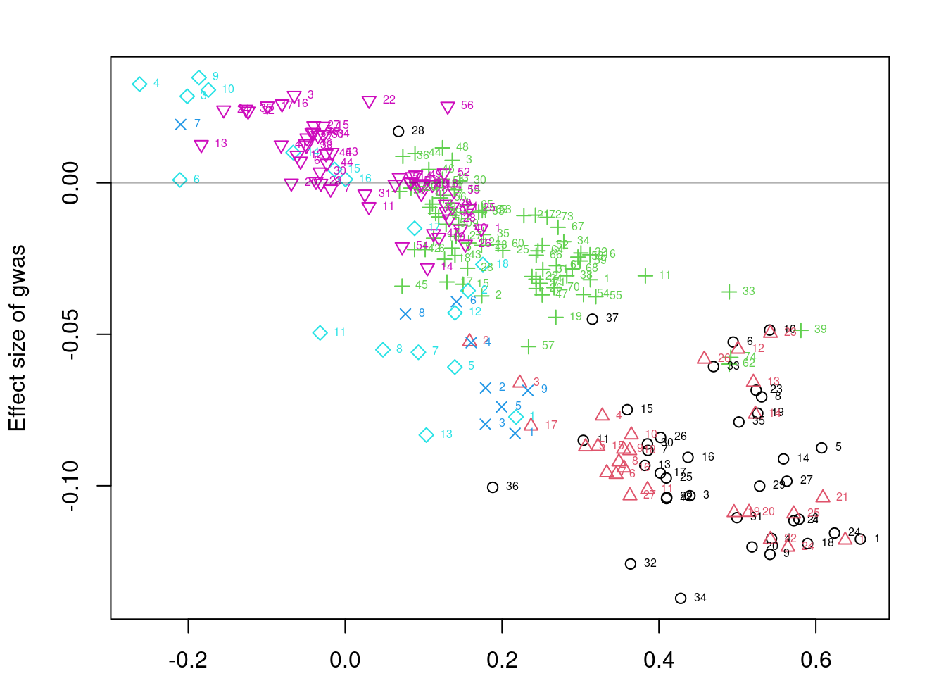

Past versions of unnamed-chunk-11-2.png

Version	Author	Date
d17186e	wesleycrouse	2023-06-08

#colocalization
coloc_fit <- list()
nclust <- length(data$beta_hat_a)

options(mc.cores=4)
for (j in 1:nclust) {
  if (length(data$beta_hat_a[[j]])>1){
    coloc_fit[[j]] <- with(data,
                           fitBetaColoc(
                             beta_hat_a = beta_hat_a[[j]],
                             beta_hat_b = beta_hat_b[[j]],
                             se_a = se_a[[j]],
                             se_b = se_b[[j]],
                             Sigma_a = Sigma[[j]],
                             Sigma_b = Sigma[[j]]
                           ))
  } else {
    coloc_fit[[j]] <- list(beta_hat_a=data$beta_hat_a[[j]],
                           beta_hat_b=data$beta_hat_b[[j]])
  }
}

Warning: There were 643 divergent transitions after warmup. See
https://mc-stan.org/misc/warnings.html#divergent-transitions-after-warmup
to find out why this is a problem and how to eliminate them.

Warning: There were 1369 transitions after warmup that exceeded the maximum treedepth. Increase max_treedepth above 10. See
https://mc-stan.org/misc/warnings.html#maximum-treedepth-exceeded

Warning: There were 2 chains where the estimated Bayesian Fraction of Missing Information was low. See
https://mc-stan.org/misc/warnings.html#bfmi-low

Warning: Examine the pairs() plot to diagnose sampling problems

Warning: Bulk Effective Samples Size (ESS) is too low, indicating posterior means and medians may be unreliable.
Running the chains for more iterations may help. See
https://mc-stan.org/misc/warnings.html#bulk-ess

Warning: Tail Effective Samples Size (ESS) is too low, indicating posterior variances and tail quantiles may be unreliable.
Running the chains for more iterations may help. See
https://mc-stan.org/misc/warnings.html#tail-ess

Warning: There were 1075 divergent transitions after warmup. See
https://mc-stan.org/misc/warnings.html#divergent-transitions-after-warmup
to find out why this is a problem and how to eliminate them.

Warning: There were 293 transitions after warmup that exceeded the maximum treedepth. Increase max_treedepth above 10. See
https://mc-stan.org/misc/warnings.html#maximum-treedepth-exceeded

Warning: There were 2 chains where the estimated Bayesian Fraction of Missing Information was low. See
https://mc-stan.org/misc/warnings.html#bfmi-low

Warning: Examine the pairs() plot to diagnose sampling problems

Warning: The largest R-hat is 1.3, indicating chains have not mixed.
Running the chains for more iterations may help. See
https://mc-stan.org/misc/warnings.html#r-hat

Warning: Bulk Effective Samples Size (ESS) is too low, indicating posterior means and medians may be unreliable.
Running the chains for more iterations may help. See
https://mc-stan.org/misc/warnings.html#bulk-ess

Warning: Tail Effective Samples Size (ESS) is too low, indicating posterior variances and tail quantiles may be unreliable.
Running the chains for more iterations may help. See
https://mc-stan.org/misc/warnings.html#tail-ess

Warning: There were 933 divergent transitions after warmup. See
https://mc-stan.org/misc/warnings.html#divergent-transitions-after-warmup
to find out why this is a problem and how to eliminate them.

Warning: There were 2576 transitions after warmup that exceeded the maximum treedepth. Increase max_treedepth above 10. See
https://mc-stan.org/misc/warnings.html#maximum-treedepth-exceeded

Warning: There were 4 chains where the estimated Bayesian Fraction of Missing Information was low. See
https://mc-stan.org/misc/warnings.html#bfmi-low

Warning: Examine the pairs() plot to diagnose sampling problems

Warning: The largest R-hat is 1.18, indicating chains have not mixed.
Running the chains for more iterations may help. See
https://mc-stan.org/misc/warnings.html#r-hat

Warning: Bulk Effective Samples Size (ESS) is too low, indicating posterior means and medians may be unreliable.
Running the chains for more iterations may help. See
https://mc-stan.org/misc/warnings.html#bulk-ess

Warning: Tail Effective Samples Size (ESS) is too low, indicating posterior variances and tail quantiles may be unreliable.
Running the chains for more iterations may help. See
https://mc-stan.org/misc/warnings.html#tail-ess

Warning: There were 428 divergent transitions after warmup. See
https://mc-stan.org/misc/warnings.html#divergent-transitions-after-warmup
to find out why this is a problem and how to eliminate them.

Warning: Examine the pairs() plot to diagnose sampling problems

Warning: Bulk Effective Samples Size (ESS) is too low, indicating posterior means and medians may be unreliable.
Running the chains for more iterations may help. See
https://mc-stan.org/misc/warnings.html#bulk-ess

Warning: Tail Effective Samples Size (ESS) is too low, indicating posterior variances and tail quantiles may be unreliable.
Running the chains for more iterations may help. See
https://mc-stan.org/misc/warnings.html#tail-ess

Warning: There were 696 divergent transitions after warmup. See
https://mc-stan.org/misc/warnings.html#divergent-transitions-after-warmup
to find out why this is a problem and how to eliminate them.

Warning: There were 2 transitions after warmup that exceeded the maximum treedepth. Increase max_treedepth above 10. See
https://mc-stan.org/misc/warnings.html#maximum-treedepth-exceeded

Warning: Examine the pairs() plot to diagnose sampling problems

Warning: The largest R-hat is 1.07, indicating chains have not mixed.
Running the chains for more iterations may help. See
https://mc-stan.org/misc/warnings.html#r-hat

Warning: Bulk Effective Samples Size (ESS) is too low, indicating posterior means and medians may be unreliable.
Running the chains for more iterations may help. See
https://mc-stan.org/misc/warnings.html#bulk-ess

Warning: Tail Effective Samples Size (ESS) is too low, indicating posterior variances and tail quantiles may be unreliable.
Running the chains for more iterations may help. See
https://mc-stan.org/misc/warnings.html#tail-ess

Warning: There were 452 divergent transitions after warmup. See
https://mc-stan.org/misc/warnings.html#divergent-transitions-after-warmup
to find out why this is a problem and how to eliminate them.

Warning: There were 3328 transitions after warmup that exceeded the maximum treedepth. Increase max_treedepth above 10. See
https://mc-stan.org/misc/warnings.html#maximum-treedepth-exceeded

Warning: There were 4 chains where the estimated Bayesian Fraction of Missing Information was low. See
https://mc-stan.org/misc/warnings.html#bfmi-low

Warning: Examine the pairs() plot to diagnose sampling problems

Warning: The largest R-hat is 1.11, indicating chains have not mixed.
Running the chains for more iterations may help. See
https://mc-stan.org/misc/warnings.html#r-hat

Warning: Bulk Effective Samples Size (ESS) is too low, indicating posterior means and medians may be unreliable.
Running the chains for more iterations may help. See
https://mc-stan.org/misc/warnings.html#bulk-ess

Warning: Tail Effective Samples Size (ESS) is too low, indicating posterior variances and tail quantiles may be unreliable.
Running the chains for more iterations may help. See
https://mc-stan.org/misc/warnings.html#tail-ess

res <- list(beta_hat_a = lapply(coloc_fit, `[[`, "beta_hat_a"),
            beta_hat_b = lapply(coloc_fit, `[[`, "beta_hat_b"),
            sd_a = data$se_a,
            sd_b = data$se_b,
            alleles = data$alleles)

res <- extractForSlope(res)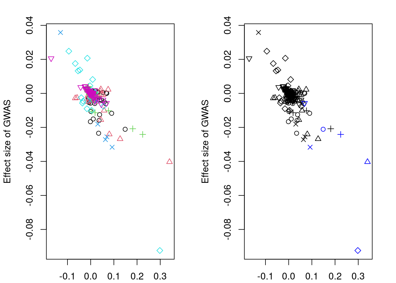

Past versions of unnamed-chunk-11-3.png

Version	Author	Date
d17186e	wesleycrouse	2023-06-08

res

$beta_hat_a
[1] 0.14875346 0.33998516 0.22431695 0.09251984 0.29819375 0.06850408

$beta_hat_b
[1] -0.021096848 -0.040317704 -0.024124520 -0.031645010 -0.092383982
[6] -0.005685927

$sd_a
[1] 0.0527500 0.0530704 0.1075950 0.0742875 0.0552440 0.0523450

$sd_b
[1] 0.011252839 0.011254246 0.019115350 0.012252449 0.009954775 0.010028221

$alleles
            id ref eff
1    rs1860471   C   T
38    rs313830   C   T
126  rs2007731   G   A
147 rs34430824   C   T
148  rs2016325   C   T
190  rs6977334   G   A

#sort clusters by significance
res$abs_z <- abs(res$beta_hat_a/res$sd_a)
res_sig_order <- order(-res$abs_z)

res$beta_hat_a <- res$beta_hat_a[res_sig_order]
res$beta_hat_b <- res$beta_hat_b[res_sig_order]
res$sd_a <- res$sd_a[res_sig_order]
res$sd_b <- res$sd_b[res_sig_order]
res$alleles <- res$alleles[res_sig_order,,drop=F]
res$abs_z <- NULL

####################

res_bkup <- res

####################

#trim clusters if (absolute) correlation greater than 0.05
if (length(res$alleles$id)>1){
  trim_index <- trimClusters(r2=abs(R_snp[res$alleles$id,res$alleles$id,drop=F]),
                             r2_threshold=0.05)

  if (length(trim_index)>0){
    res$beta_hat_a <- res$beta_hat_a[-trim_index]
    res$beta_hat_b <- res$beta_hat_b[-trim_index]
    res$sd_a <- res$sd_a[-trim_index]
    res$sd_b <- res$sd_b[-trim_index]
    res$alleles <- res$alleles[-trim_index,,drop=F]
  }
}

####################
#visual input data

par(mfrow=c(3,1))

logging::loginfo(gene)

2023-06-12 15:44:06 INFO::ENSG00000237310

par(mar=c(2.1, 4.1, 2.1, 2.1))

plot(df_locus$pos, abs(df_locus$z_gwas), xlab="", ylab="GWAS |Z|")
abline(v=df_locus$pos[df_locus$causal], col="red")

plot(df_locus$pos, abs(df_locus$z_eqtl), xlab="", ylab="eQTL SS |Z|",
     col=colors[df_locus$clump+1])
abline(v=df_locus$pos[df_locus$causal], col="red")

plot(df_locus$pos, abs(df_locus$weight), col="purple", xlab="", ylab="eQTL Lasso |wgt|")
abline(v=df_locus$pos[df_locus$causal], col="red")

breakpoints <- ld_R_info[ld_R_info$index!=c(ld_R_info$index[-1],max(ld_R_info$index)),]
breakpoints <- breakpoints[breakpoints$chrom==chr,]
breakpoints <- breakpoints[breakpoints$pos>min(df_locus$pos) & breakpoints$pos<max(df_locus$pos),]

abline(v=breakpoints$pos)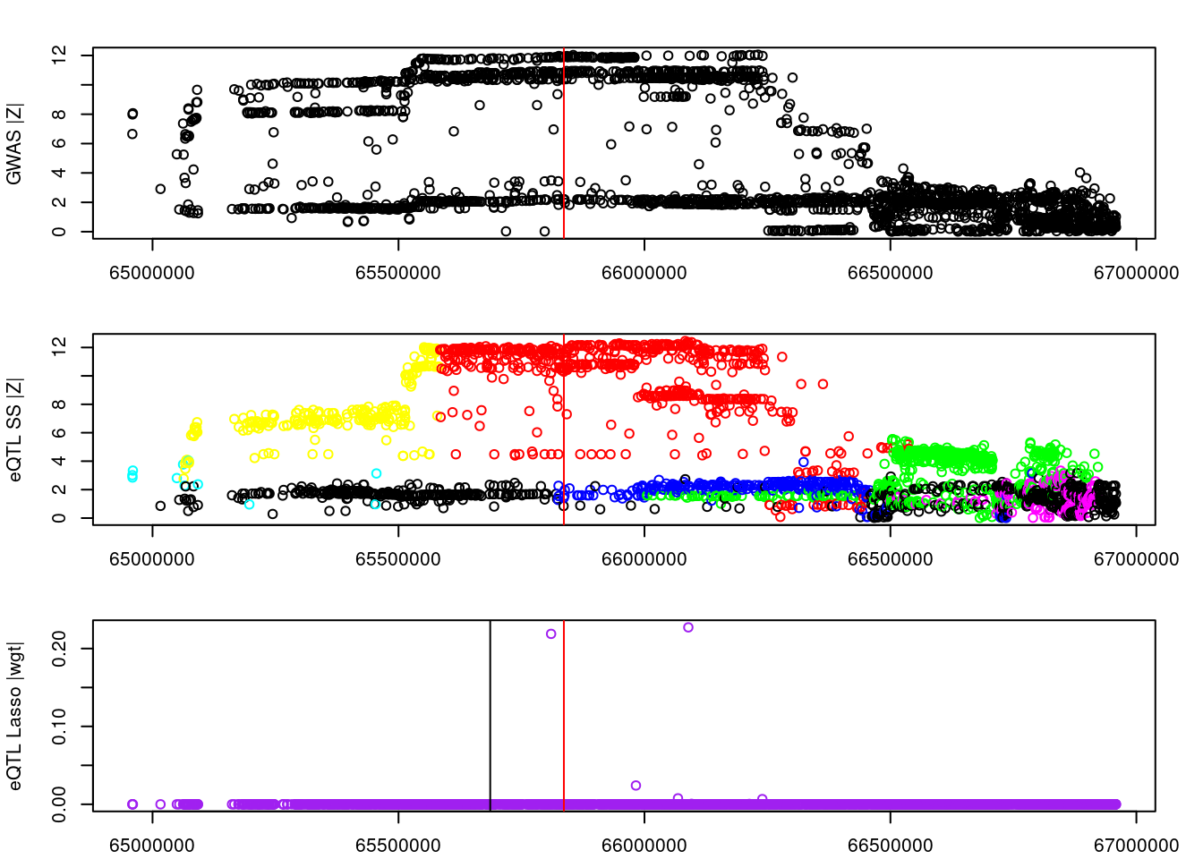

Past versions of unnamed-chunk-11-4.png

Version	Author	Date
d17186e	wesleycrouse	2023-06-08

df_locus$trim <- F
df_locus$trim[match(res_bkup$alleles$id[trim_index], df_locus$id)] <- T
df_locus$color <- colors[df_locus$clump+1]
df_locus[match(res_bkup$alleles$id, df_locus$id),]

                id    z_eqtl chrom      pos      z_gwas causal weight clump
5526878   rs313830 12.010801     7 65551931 -10.4780020  FALSE      0     2
5528329  rs2016325  3.941677     7 66323500  -7.7619339  FALSE      0     5
5527837  rs1860471 12.451166     7 66082946 -10.4516260  FALSE      0     1
5530252  rs2007731 -4.550797     7 66825873   3.1294781  FALSE      0     3
5530376  rs6977334 -3.016926     7 66848202   0.8392996  FALSE      0     6
5526686 rs34430824  3.135588     7 65455084  -5.5923938  FALSE      0     4
         trim   color
5526878 FALSE #FFFF00
5528329  TRUE #0000FF
5527837  TRUE #FF0000
5530252  TRUE #00FF00
5530376  TRUE #FF00FF
5526686  TRUE #00FFFF

par(mfrow=c(1,1))

scales::show_col(colors[c(1, res_sig_order+1)])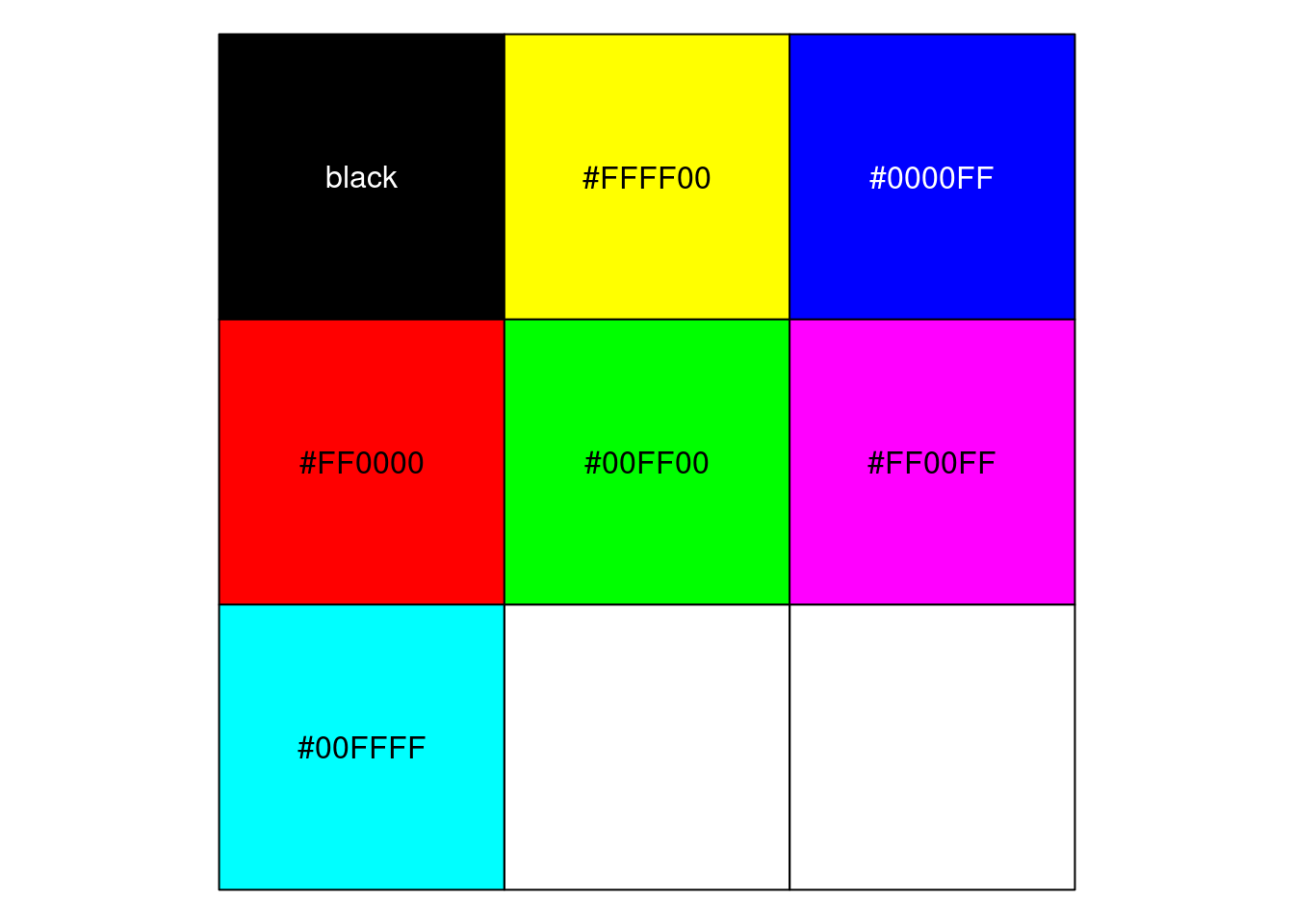

Past versions of unnamed-chunk-11-5.png

Version	Author	Date
d17186e	wesleycrouse	2023-06-08

####################

if (length(res$beta_hat_a)==1){
  #parametric sample from MRLocus code
  m <- 1e+05
  post_samples <- list(alpha=rnorm(m, res$beta_hat_b, res$sd_b)/rnorm(m, res$beta_hat_a, res$sd_a))
} else {
  #fit MRLocus slope model
  res <- fitSlope(res, iter=10000)
  post_samples <- rstan::extract(res$stanfit)
}

par(mfrow=c(1,1))

#display results
print(res$stanfit, pars=c("alpha","sigma"), probs=c(.1,.9), digits=3)

NULL

if (!is.null(res$stanfit)){
  plotMrlocus(res, main="MRLocus gene-to-trait effect estimate")
} else {
  logging::loginfo("<2 clumps for analysis")
}

2023-06-12 15:44:06 INFO::<2 clumps for analysis

####################
#investigate LD between confounding variants and eSNPs for clumps

#confounding causal SNPs
df_locus[df_locus$causal,]

              id    z_eqtl chrom      pos   z_gwas causal weight clump  trim
5527360 rs778685 -10.57407     7 65836176 11.90402   TRUE      0     1 FALSE
          color
5527360 #FF0000

#eSNPs in the analysis
df_locus[match(res$alleles$id, df_locus$id),]

              id  z_eqtl chrom      pos  z_gwas causal weight clump  trim
5526878 rs313830 12.0108     7 65551931 -10.478  FALSE      0     2 FALSE
          color
5526878 #FFFF00

#LD between confounding SNPs and eSNPs
snplist_all <- c(df_locus$id[df_locus$causal], res$alleles$id)

ld_R_idx <- unique(ld_R_info$index[match(snplist_all, ld_R_info$id)])

R_snp <- lapply(ld_R_files[ld_R_idx], readRDS)

R_snp_info <- lapply(ld_R_info_files[ld_R_idx], fread)
R_snp_info <- lapply(R_snp_info, as.data.frame)

R_snp_index <- lapply(R_snp_info, function(x){x$id %in% snplist_all})

for (j in 1:length(R_snp)){
  R_snp[[j]] <- R_snp[[j]][R_snp_index[[j]],R_snp_index[[j]]]
  R_snp_info[[j]] <- R_snp_info[[j]][R_snp_index[[j]],,drop=F]
}

R_snp_info <- as.data.frame(do.call(rbind, R_snp_info))
R_snp <- as.matrix(Matrix::bdiag(R_snp))

colnames(R_snp) <- R_snp_info$id
rownames(R_snp) <- R_snp_info$id

#number of LD regions
length(ld_R_idx)

[1] 2

#LD between variants
R_snp[snplist_all, snplist_all]

         rs778685 rs313830
rs778685        1        0
rs313830        0        1

Session information

sessionInfo()

R version 4.1.0 (2021-05-18)
Platform: x86_64-pc-linux-gnu (64-bit)
Running under: CentOS Linux 7 (Core)

Matrix products: default
BLAS:   /software/R-4.1.0-no-openblas-el7-x86_64/lib64/R/lib/libRblas.so
LAPACK: /software/R-4.1.0-no-openblas-el7-x86_64/lib64/R/lib/libRlapack.so

locale:
 [1] LC_CTYPE=en_US.UTF-8 LC_NUMERIC=C         LC_TIME=C           
 [4] LC_COLLATE=C         LC_MONETARY=C        LC_MESSAGES=C       
 [7] LC_PAPER=C           LC_NAME=C            LC_ADDRESS=C        
[10] LC_TELEPHONE=C       LC_MEASUREMENT=C     LC_IDENTIFICATION=C 

attached base packages:
[1] stats     graphics  grDevices utils     datasets  methods   base     

other attached packages:
[1] ctwas_0.1.34      mrlocus_0.0.25    data.table_1.14.6 workflowr_1.7.0  

loaded via a namespace (and not attached):
 [1] Rcpp_1.0.9           lattice_0.20-45      prettyunits_1.1.1   
 [4] getPass_0.2-2        ps_1.7.2             foreach_1.5.2       
 [7] assertthat_0.2.1     rprojroot_2.0.3      digest_0.6.31       
[10] utf8_1.2.2           R6_2.5.1             RcppZiggurat_0.1.6  
[13] stats4_4.1.0         evaluate_0.18        highr_0.9           
[16] httr_1.4.4           ggplot2_3.4.0        pillar_1.8.1        
[19] rlang_1.0.6          rstudioapi_0.14      whisker_0.4.1       
[22] callr_3.7.3          jquerylib_0.1.4      Matrix_1.5-3        
[25] rmarkdown_2.18       stringr_1.5.0        loo_2.5.1           
[28] munsell_0.5.0        compiler_4.1.0       httpuv_1.6.6        
[31] xfun_0.35            rstan_2.21.7         pkgconfig_2.0.3     
[34] pkgbuild_1.4.0       htmltools_0.5.4      tidyselect_1.2.0    
[37] tibble_3.1.8         gridExtra_2.3        logging_0.10-108    
[40] codetools_0.2-18     matrixStats_0.63.0   fansi_1.0.3         
[43] withr_2.5.0          crayon_1.5.2         dplyr_1.0.10        
[46] later_1.3.0          MASS_7.3-58.1        grid_4.1.0          
[49] jsonlite_1.8.4       gtable_0.3.1         lifecycle_1.0.3     
[52] DBI_1.1.3            git2r_0.30.1         magrittr_2.0.3      
[55] StanHeaders_2.21.0-7 scales_1.2.1         Rfast_2.0.6         
[58] RcppParallel_5.1.5   cli_3.4.1            stringi_1.7.8       
[61] cachem_1.0.6         farver_2.1.1         fs_1.5.2            
[64] promises_1.2.0.1     pgenlibr_0.3.2       bslib_0.4.1         
[67] vctrs_0.5.1          generics_0.1.3       iterators_1.0.14    
[70] tools_4.1.0          glue_1.6.2           processx_3.8.0      
[73] parallel_4.1.0       fastmap_1.1.0        yaml_2.3.6          
[76] inline_0.3.19        colorspace_2.0-3     knitr_1.41          
[79] sass_0.4.4