Schizophrenia - all weights (no lncRNA) - corrected
wesleycrouse
2022-02-28
Last updated: 2022-10-03
Checks: 6 1
Knit directory: ctwas_applied/
This reproducible R Markdown analysis was created with workflowr (version 1.6.2). The Checks tab describes the reproducibility checks that were applied when the results were created. The Past versions tab lists the development history.
The R Markdown file has unstaged changes. To know which version of the R Markdown file created these results, you’ll want to first commit it to the Git repo. If you’re still working on the analysis, you can ignore this warning. When you’re finished, you can run wflow_publish to commit the R Markdown file and build the HTML.
Great job! The global environment was empty. Objects defined in the global environment can affect the analysis in your R Markdown file in unknown ways. For reproduciblity it’s best to always run the code in an empty environment.
The command set.seed(20210726) was run prior to running the code in the R Markdown file. Setting a seed ensures that any results that rely on randomness, e.g. subsampling or permutations, are reproducible.
Great job! Recording the operating system, R version, and package versions is critical for reproducibility.
Nice! There were no cached chunks for this analysis, so you can be confident that you successfully produced the results during this run.
Great job! Using relative paths to the files within your workflowr project makes it easier to run your code on other machines.
Great! You are using Git for version control. Tracking code development and connecting the code version to the results is critical for reproducibility.
The results in this page were generated with repository version 7526db7. See the Past versions tab to see a history of the changes made to the R Markdown and HTML files.
Note that you need to be careful to ensure that all relevant files for the analysis have been committed to Git prior to generating the results (you can use wflow_publish or wflow_git_commit). workflowr only checks the R Markdown file, but you know if there are other scripts or data files that it depends on. Below is the status of the Git repository when the results were generated:
Untracked files:
    Untracked:  workspace1.RData
    Untracked:  workspace2.RData
    Untracked:  workspace20.RData
    Untracked:  workspace3.RData
    Untracked:  z_snp_pos_ebi-a-GCST004131.RData
    Untracked:  z_snp_pos_ebi-a-GCST004132.RData
    Untracked:  z_snp_pos_ebi-a-GCST004133.RData
    Untracked:  z_snp_pos_scz-2018.RData
    Untracked:  z_snp_pos_ukb-a-360.RData
    Untracked:  z_snp_pos_ukb-d-30780_irnt.RData

Unstaged changes:
    Modified:   analysis/scz-2018_allweights_nolnc_corrected.Rmd
Note that any generated files, e.g. HTML, png, CSS, etc., are not included in this status report because it is ok for generated content to have uncommitted changes.
These are the previous versions of the repository in which changes were made to the R Markdown (analysis/scz-2018_allweights_nolnc_corrected.Rmd) and HTML (docs/scz-2018_allweights_nolnc_corrected.html) files. If you’ve configured a remote Git repository (see ?wflow_git_remote), click on the hyperlinks in the table below to view the files as they were in that past version.
| File | Version | Author | Date | Message |
|---|---|---|---|---|
| Rmd | 7526db7 | wesleycrouse | 2022-10-03 | preparing to transition SCZ silver standarad |
| html | 7526db7 | wesleycrouse | 2022-10-03 | preparing to transition SCZ silver standarad |
| Rmd | eb3c5bf | wesleycrouse | 2022-09-27 | regenerating tables |
| html | eb3c5bf | wesleycrouse | 2022-09-27 | regenerating tables |
| html | 3349d12 | wesleycrouse | 2022-09-16 | maybe final tables |
| Rmd | 6a57156 | wesleycrouse | 2022-09-14 | regenerating tables |
| html | 6a57156 | wesleycrouse | 2022-09-14 | regenerating tables |
| Rmd | 220ba1d | wesleycrouse | 2022-09-09 | figure revisions |
| html | 220ba1d | wesleycrouse | 2022-09-09 | figure revisions |
| Rmd | 2af4567 | wesleycrouse | 2022-09-02 | working on supplemental figures |
| html | 2af4567 | wesleycrouse | 2022-09-02 | working on supplemental figures |
| Rmd | 0b519f1 | wesleycrouse | 2022-07-28 | relaxing GO silver threshold for SBP and SCZ |
| html | 0b519f1 | wesleycrouse | 2022-07-28 | relaxing GO silver threshold for SBP and SCZ |
| Rmd | c19144f | wesleycrouse | 2022-07-28 | sorting GO results |
| html | c19144f | wesleycrouse | 2022-07-28 | sorting GO results |
| Rmd | 0f5b69a | wesleycrouse | 2022-07-28 | output silver standard GO and MAGMA |
| html | 0f5b69a | wesleycrouse | 2022-07-28 | output silver standard GO and MAGMA |
| Rmd | cb3f976 | wesleycrouse | 2022-07-27 | SCZ and SBP magma results |
| html | cb3f976 | wesleycrouse | 2022-07-27 | SCZ and SBP magma results |
| Rmd | dd9f346 | wesleycrouse | 2022-07-27 | regenerate plots |
| html | dd9f346 | wesleycrouse | 2022-07-27 | regenerate plots |
| Rmd | 0803b64 | wesleycrouse | 2022-07-27 | testing figure titles |
| Rmd | 7474fef | wesleycrouse | 2022-07-26 | SCZ testing |
| html | 7474fef | wesleycrouse | 2022-07-26 | SCZ testing |
| Rmd | 9ad1d4f | wesleycrouse | 2022-07-26 | SCZ MESC results |
| html | 9ad1d4f | wesleycrouse | 2022-07-26 | SCZ MESC results |
| Rmd | f2cc313 | wesleycrouse | 2022-07-25 | SCZ fix |
| html | f2cc313 | wesleycrouse | 2022-07-25 | SCZ fix |
| Rmd | 9e83da3 | wesleycrouse | 2022-07-25 | SCZ silver standard |
| html | 9e83da3 | wesleycrouse | 2022-07-25 | SCZ silver standard |
| Rmd | 3be2b06 | wesleycrouse | 2022-07-25 | SBP silver standard |
| Rmd | 00feffc | wesleycrouse | 2022-07-19 | forgot the analysis file |
| Rmd | 4ee76a3 | wesleycrouse | 2022-07-19 | SBP and IBD fixes for novel genes |
| html | 4ee76a3 | wesleycrouse | 2022-07-19 | SBP and IBD fixes for novel genes |
| Rmd | d34b3a0 | wesleycrouse | 2022-07-19 | tinkering with plots |
| html | d34b3a0 | wesleycrouse | 2022-07-19 | tinkering with plots |
| Rmd | 4ded2ef | wesleycrouse | 2022-07-19 | SBP and SCZ results |
| html | 4ded2ef | wesleycrouse | 2022-07-19 | SBP and SCZ results |
| Rmd | 772879d | wesleycrouse | 2022-07-14 | final IBD plot prep |
options(width=1000)trait_id <- "scz-2018"
trait_name <- "Schizophrenia"
source("/project2/mstephens/wcrouse/UKB_analysis_allweights_scz/ctwas_config.R")
trait_dir <- paste0("/project2/mstephens/wcrouse/UKB_analysis_allweights_scz/", trait_id)
results_dirs <- list.dirs(trait_dir, recursive=F)Load cTWAS results for all weights
# df <- list()
#
# for (i in 1:length(results_dirs)){
#   print(i)
#
#   results_dir <- results_dirs[i]
#   weight <- rev(unlist(strsplit(results_dir, "/")))[1]
#   weight <- unlist(strsplit(weight, split="_nolnc"))
#   analysis_id <- paste(trait_id, weight, sep="_")
#
#   #load ctwas results
#   ctwas_res <- data.table::fread(paste0(results_dir, "/", analysis_id, "_ctwas.susieIrss.txt"))
#
#   #make unique identifier for regions and effects
#   ctwas_res$region_tag <- paste(ctwas_res$region_tag1, ctwas_res$region_tag2, sep="_")
#   ctwas_res$region_cs_tag <- paste(ctwas_res$region_tag, ctwas_res$cs_index, sep="_")
#
#   #load z scores for SNPs and collect sample size
#   load(paste0(results_dir, "/", analysis_id, "_expr_z_snp.Rd"))
#
#   sample_size <- z_snp$ss
#   sample_size <- as.numeric(names(which.max(table(sample_size))))
#
#   #compute PVE for each gene/SNP
#   ctwas_res$PVE = ctwas_res$susie_pip*ctwas_res$mu2/sample_size
#
#   #separate gene and SNP results
#   ctwas_gene_res <- ctwas_res[ctwas_res$type == "gene", ]
#   ctwas_gene_res <- data.frame(ctwas_gene_res)
#   ctwas_snp_res <- ctwas_res[ctwas_res$type == "SNP", ]
#   ctwas_snp_res <- data.frame(ctwas_snp_res)
#
#   #add gene information to results
#   sqlite <- RSQLite::dbDriver("SQLite")
#   db = RSQLite::dbConnect(sqlite, paste0("/project2/mstephens/wcrouse/predictdb_nolnc/mashr_", weight, "_nolnc.db"))
#   query <- function(...) RSQLite::dbGetQuery(db, ...)
#   gene_info <- query("select gene, genename, gene_type from extra")
#   RSQLite::dbDisconnect(db)
#
#   ctwas_gene_res <- cbind(ctwas_gene_res, gene_info[sapply(ctwas_gene_res$id, match, gene_info$gene), c("genename", "gene_type")])
#
#   #add z scores to results
#   load(paste0(results_dir, "/", analysis_id, "_expr_z_gene.Rd"))
#   ctwas_gene_res$z <- z_gene[ctwas_gene_res$id,]$z
#
#   z_snp <- z_snp[z_snp$id %in% ctwas_snp_res$id,]
#   ctwas_snp_res$z <- z_snp$z[match(ctwas_snp_res$id, z_snp$id)]
#
#   #merge gene and snp results with added information
#   ctwas_snp_res$genename=NA
#   ctwas_snp_res$gene_type=NA
#
#   ctwas_res <- rbind(ctwas_gene_res, ctwas_snp_res[,colnames(ctwas_gene_res)])
#
#   #get number of eQTL for genes
#   num_eqtl <- c()
#   for (i in 1:22){
#     load(paste0(results_dir, "/", analysis_id, "_expr_chr", i, ".exprqc.Rd"))
#     num_eqtl <- c(num_eqtl, unlist(lapply(wgtlist, nrow)))
#   }
#   ctwas_gene_res$num_eqtl <- num_eqtl[ctwas_gene_res$id]
#
#   #get number of SNPs from s1 results; adjust for thin argument
#   ctwas_res_s1 <- data.table::fread(paste0(results_dir, "/", analysis_id, "_ctwas.s1.susieIrss.txt"))
#   n_snps <- sum(ctwas_res_s1$type=="SNP")/thin
#   rm(ctwas_res_s1)
#
#   #load estimated parameters
#   load(paste0(results_dir, "/", analysis_id, "_ctwas.s2.susieIrssres.Rd"))
#
#   #estimated group prior
#   estimated_group_prior <- group_prior_rec[,ncol(group_prior_rec)]
#   names(estimated_group_prior) <- c("gene", "snp")
#   estimated_group_prior["snp"] <- estimated_group_prior["snp"]*thin #adjust parameter to account for thin argument
#
#   #estimated group prior variance
#   estimated_group_prior_var <- group_prior_var_rec[,ncol(group_prior_var_rec)]
#   names(estimated_group_prior_var) <- c("gene", "snp")
#
#   #report group size
#   group_size <- c(nrow(ctwas_gene_res), n_snps)
#
#   #estimated group PVE
#   estimated_group_pve <- estimated_group_prior_var*estimated_group_prior*group_size/sample_size
#   names(estimated_group_pve) <- c("gene", "snp")
#
#   #ctwas genes using PIP>0.8
#   ctwas_genes_index <- ctwas_gene_res$susie_pip>0.8
#   ctwas_genes <- ctwas_gene_res$genename[ctwas_genes_index]
#
#   #twas genes using bonferroni threshold
#   alpha <- 0.05
#   sig_thresh <- qnorm(1-(alpha/nrow(ctwas_gene_res)/2), lower=T)
#
#   twas_genes_index <- abs(ctwas_gene_res$z) > sig_thresh
#   twas_genes <- ctwas_gene_res$genename[twas_genes_index]
#
#   #gene PIPs and z scores
#   gene_pips <- ctwas_gene_res[,c("genename", "region_tag", "susie_pip", "z", "region_cs_tag", "num_eqtl")]
#
#   #total PIPs by region
#   regions <- unique(ctwas_gene_res$region_tag)
#   region_pips <- data.frame(region=regions, stringsAsFactors=F)
#   region_pips$gene_pip <- sapply(regions, function(x){sum(ctwas_gene_res$susie_pip[ctwas_gene_res$region_tag==x])})
#   region_pips$snp_pip <- sapply(regions, function(x){sum(ctwas_snp_res$susie_pip[ctwas_snp_res$region_tag==x])})
#   region_pips$snp_maxz <- sapply(regions, function(x){max(abs(ctwas_snp_res$z[ctwas_snp_res$region_tag==x]))})
#   region_pips$which_snp_maxz <- sapply(regions, function(x){ctwas_snp_res_index <- ctwas_snp_res$region_tag==x; ctwas_snp_res$id[ctwas_snp_res_index][which.max(abs(ctwas_snp_res$z[ctwas_snp_res_index]))]})
#
#   #total PIPs by causal set
#   regions_cs <- unique(ctwas_gene_res$region_cs_tag)
#   region_cs_pips <- data.frame(region_cs=regions_cs, stringsAsFactors=F)
#   region_cs_pips$gene_pip <- sapply(regions_cs, function(x){sum(ctwas_gene_res$susie_pip[ctwas_gene_res$region_cs_tag==x])})
#   region_cs_pips$snp_pip <- sapply(regions_cs, function(x){sum(ctwas_snp_res$susie_pip[ctwas_snp_res$region_cs_tag==x])})
#
#   df[[weight]] <- list(prior=estimated_group_prior,
#                      prior_var=estimated_group_prior_var,
#                      pve=estimated_group_pve,
#                      ctwas=ctwas_genes,
#                      twas=twas_genes,
#                      gene_pips=gene_pips,
#                      region_pips=region_pips,
#                      sig_thresh=sig_thresh,
#                      region_cs_pips=region_cs_pips)
#
#   ##########
#
#   ctwas_gene_res_out <- ctwas_gene_res[,c("id", "genename", "chrom", "pos", "region_tag", "cs_index", "susie_pip", "mu2", "PVE", "z", "num_eqtl")]
#   ctwas_gene_res_out <- dplyr::rename(ctwas_gene_res_out, PIP="susie_pip", tau2="mu2")
#
#   write.csv(ctwas_gene_res_out, file=paste0("output/full_gene_results/SCZ_", weight,".csv"), row.names=F)
# }
#
# save(df, file=paste(trait_dir, "results_df_nolnc.RData", sep="/"))
load(paste(trait_dir, "results_df_nolnc.RData", sep="/"))

output <- data.frame(weight=names(df),
                     prior_g=unlist(lapply(df, function(x){x$prior["gene"]})),
                     prior_s=unlist(lapply(df, function(x){x$prior["snp"]})),
                     prior_var_g=unlist(lapply(df, function(x){x$prior_var["gene"]})),
                     prior_var_s=unlist(lapply(df, function(x){x$prior_var["snp"]})),
                     pve_g=unlist(lapply(df, function(x){x$pve["gene"]})),
                     pve_s=unlist(lapply(df, function(x){x$pve["snp"]})),
                     n_ctwas=unlist(lapply(df, function(x){length(x$ctwas)})),
                     n_twas=unlist(lapply(df, function(x){length(x$twas)})),
                     row.names=NULL,
                     stringsAsFactors=F)
Plot estimated prior parameters and PVE
#plot estimated group prior

output <- output[order(-output$prior_g),]

par(mar=c(10.1, 4.1, 4.1, 2.1))

plot(output$prior_g, type="l", ylim=c(0, max(output$prior_g, output$prior_s)*1.1),
     xlab="", ylab="Estimated Group Prior", xaxt = "n", col="blue")
lines(output$prior_s)

axis(1, at = 1:nrow(output),
     labels = output$weight,
     las=2,
     cex.axis=0.6)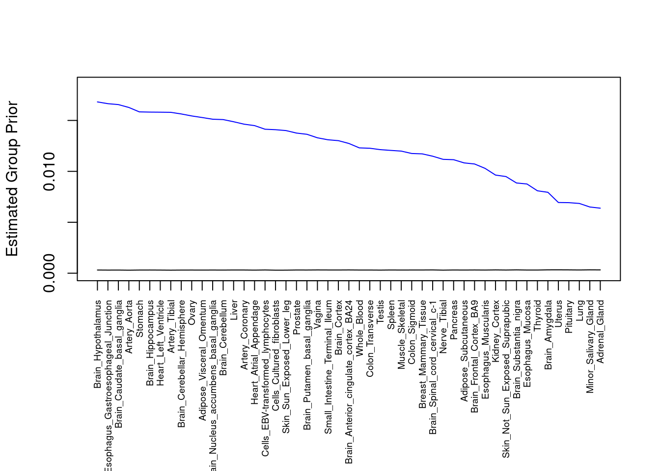
| Version | Author | Date |
|---|---|---|
| 4ded2ef | wesleycrouse | 2022-07-19 |
####################
#plot estimated group prior variance

par(mar=c(10.1, 4.1, 4.1, 2.1))

plot(output$prior_var_g, type="l", ylim=c(0, max(output$prior_var_g, output$prior_var_s)*1.1),
     xlab="", ylab="Estimated Group Prior Variance", xaxt = "n", col="blue")
lines(output$prior_var_s)

axis(1, at = 1:nrow(output),
     labels = output$weight,
     las=2,
     cex.axis=0.6)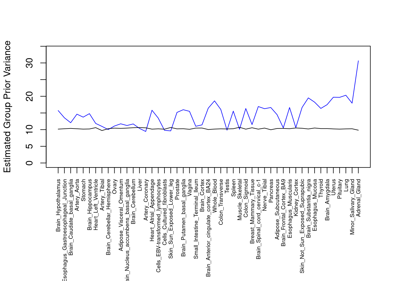
| Version | Author | Date |
|---|---|---|
| 4ded2ef | wesleycrouse | 2022-07-19 |
####################
#plot PVE

output <- output[order(-output$pve_g),]

par(mar=c(10.1, 4.1, 4.1, 2.1))

plot(output$pve_g, type="l", ylim=c(0, max(output$pve_g+output$pve_s)*1.1),
     xlab="", ylab="Estimated PVE", xaxt = "n", col="blue")
lines(output$pve_s)
lines(output$pve_g+output$pve_s, lty=2)

axis(1, at = 1:nrow(output),
     labels = output$weight,
     las=2,
     cex.axis=0.6)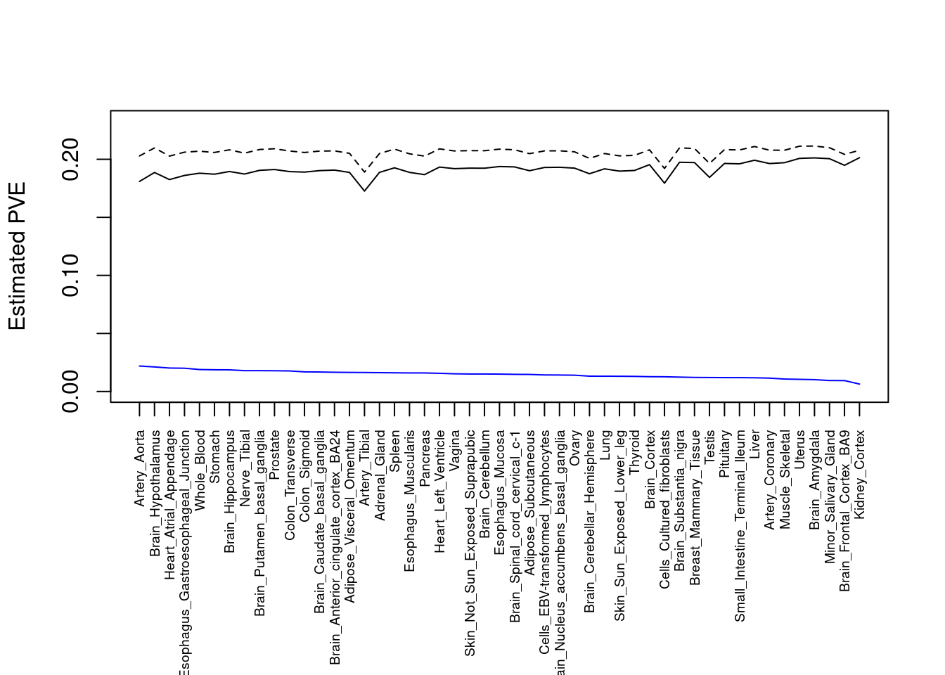
| Version | Author | Date |
|---|---|---|
| 4ded2ef | wesleycrouse | 2022-07-19 |
Number of cTWAS and TWAS genes
cTWAS genes are the set of genes with PIP>0.8 in any tissue. TWAS genes are the set of genes with significant z score (Bonferroni within tissue) in any tissue.
#plot number of significant cTWAS and TWAS genes in each tissue
plot(output$n_ctwas, output$n_twas, xlab="Number of cTWAS Genes", ylab="Number of TWAS Genes")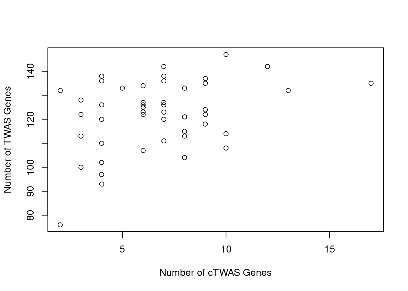
| Version | Author | Date |
|---|---|---|
| 4ded2ef | wesleycrouse | 2022-07-19 |
#number of ctwas_genes
ctwas_genes <- unique(unlist(lapply(df, function(x){x$ctwas})))
length(ctwas_genes)
[1] 104#number of twas_genes
twas_genes <- unique(unlist(lapply(df, function(x){x$twas})))
length(twas_genes)[1] 583Enrichment analysis for cTWAS genes
GO
#enrichment for cTWAS genes using enrichR
library(enrichR)
Welcome to enrichR
Checking connection ... Enrichr ... Connection is Live!
FlyEnrichr ... Connection is available!
WormEnrichr ... Connection is available!
YeastEnrichr ... Connection is available!
FishEnrichr ... Connection is available!dbs <- c("GO_Biological_Process_2021", "GO_Cellular_Component_2021", "GO_Molecular_Function_2021")
GO_enrichment <- enrichr(ctwas_genes, dbs)Uploading data to Enrichr... Done.
Querying GO_Biological_Process_2021... Done.
Querying GO_Cellular_Component_2021... Done.
Querying GO_Molecular_Function_2021... Done.
Parsing results... Done.for (db in dbs){
cat(paste0(db, "\n\n"))
enrich_results <- GO_enrichment[[db]]
enrich_results <- enrich_results[enrich_results$Adjusted.P.value<0.05,c("Term", "Overlap", "Adjusted.P.value", "Genes"), drop=F]
print(enrich_results)
print(plotEnrich(GO_enrichment[[db]]))
}GO_Biological_Process_2021
[1] Term Overlap Adjusted.P.value Genes
<0 rows> (or 0-length row.names)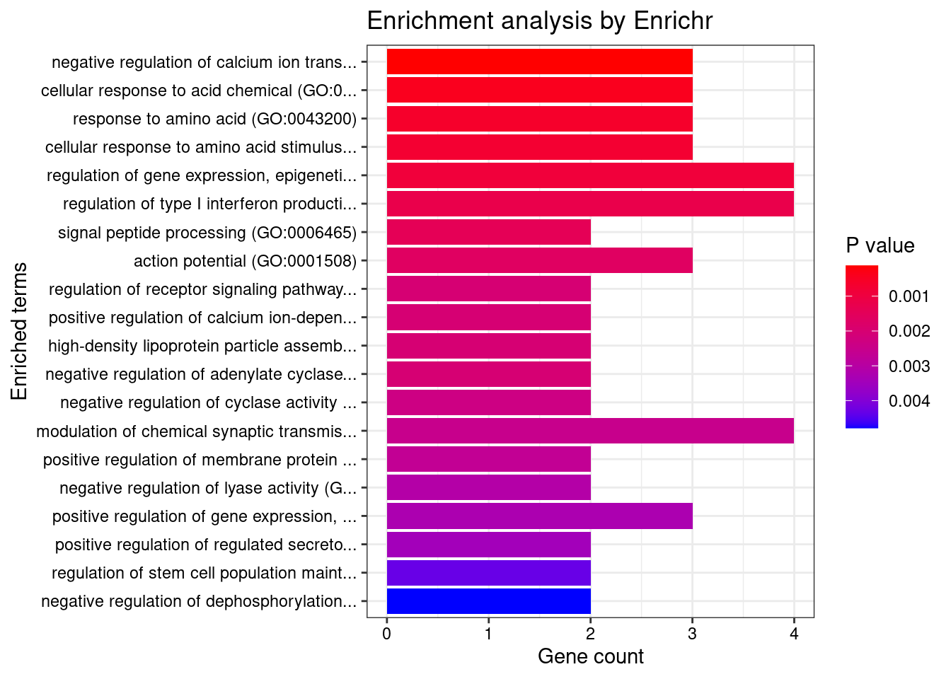
| Version | Author | Date |
|---|---|---|
| 4ded2ef | wesleycrouse | 2022-07-19 |
GO_Cellular_Component_2021
[1] Term Overlap Adjusted.P.value Genes
<0 rows> (or 0-length row.names)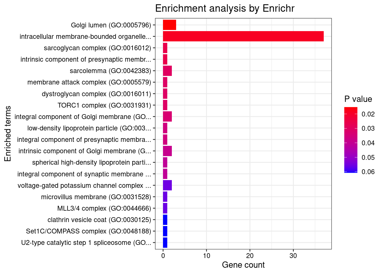
| Version | Author | Date |
|---|---|---|
| 4ded2ef | wesleycrouse | 2022-07-19 |
GO_Molecular_Function_2021
[1] Term Overlap Adjusted.P.value Genes
<0 rows> (or 0-length row.names)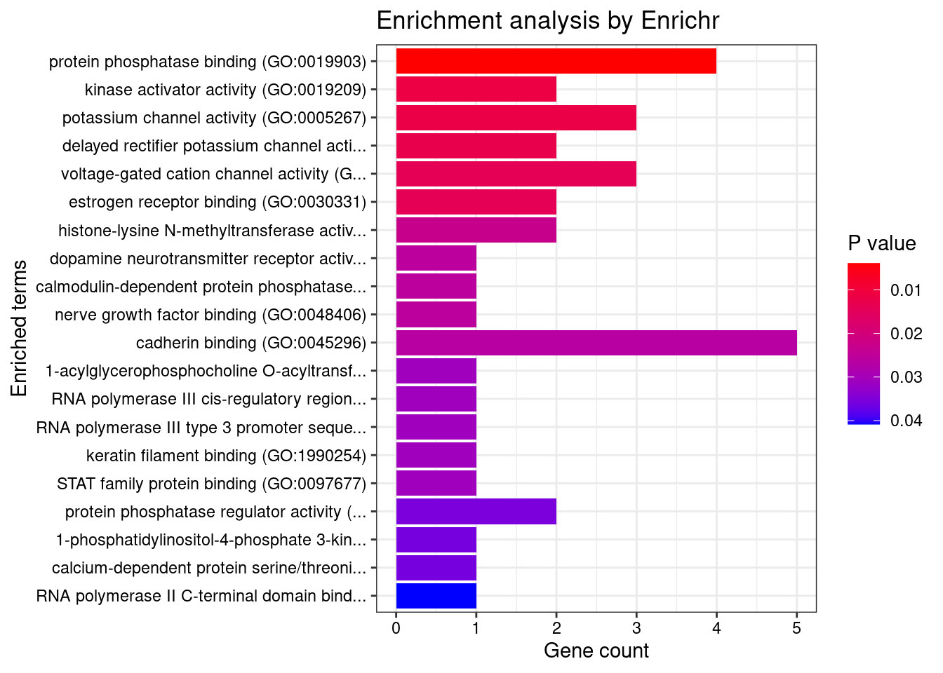
| Version | Author | Date |
|---|---|---|
| 4ded2ef | wesleycrouse | 2022-07-19 |
KEGG
#enrichment for cTWAS genes using KEGG
library(WebGestaltR)******************************************* ** Welcome to WebGestaltR ! ** *******************************************background <- unique(unlist(lapply(df, function(x){x$gene_pips$genename})))
#listGeneSet()
databases <- c("pathway_KEGG")
enrichResult <- WebGestaltR(enrichMethod="ORA", organism="hsapiens",
interestGene=ctwas_genes, referenceGene=background,
enrichDatabase=databases, interestGeneType="genesymbol",
referenceGeneType="genesymbol", isOutput=F)Loading the functional categories...
Loading the ID list...
Loading the reference list...
Performing the enrichment analysis...Warning in oraEnrichment(interestGeneList, referenceGeneList, geneSet, minNum = minNum, : No significant gene set is identified based on FDR 0.05!enrichResult[,c("description", "size", "overlap", "FDR", "userId")]NULLDisGeNET
#enrichment for cTWAS genes using DisGeNET
# devtools::install_bitbucket("ibi_group/disgenet2r")
library(disgenet2r)
disgenet_api_key <- get_disgenet_api_key(
email = "wesleycrouse@gmail.com",
password = "uchicago1" )
Sys.setenv(DISGENET_API_KEY= disgenet_api_key)
res_enrich <- disease_enrichment(entities=ctwas_genes, vocabulary = "HGNC", database = "CURATED")
if (any(res_enrich@qresult$FDR < 0.05)){
print(res_enrich@qresult[res_enrich@qresult$FDR < 0.05, c("Description", "FDR", "Ratio", "BgRatio")])
}Gene sets curated by Macarthur Lab
gene_set_dir <- "/project2/mstephens/wcrouse/gene_sets/"
gene_set_files <- c("gwascatalog.tsv",
"mgi_essential.tsv",
"core_essentials_hart.tsv",
"clinvar_path_likelypath.tsv",
"fda_approved_drug_targets.tsv")
gene_sets <- lapply(gene_set_files, function(x){as.character(read.table(paste0(gene_set_dir, x))[,1])})
names(gene_sets) <- sapply(gene_set_files, function(x){unlist(strsplit(x, "[.]"))[1]})
gene_lists <- list(ctwas_genes=ctwas_genes)
#background is union of genes analyzed in all tissue
background <- unique(unlist(lapply(df, function(x){x$gene_pips$genename})))
#genes in gene_sets filtered to ensure inclusion in background
gene_sets <- lapply(gene_sets, function(x){x[x %in% background]})
####################
hyp_score <- data.frame()
size <- c()
ngenes <- c()
for (i in 1:length(gene_sets)) {
for (j in 1:length(gene_lists)){
group1 <- length(gene_sets[[i]])
group2 <- length(as.vector(gene_lists[[j]]))
size <- c(size, group1)
Overlap <- length(intersect(gene_sets[[i]],as.vector(gene_lists[[j]])))
ngenes <- c(ngenes, Overlap)
Total <- length(background)
hyp_score[i,j] <- phyper(Overlap-1, group2, Total-group2, group1,lower.tail=F)
}
}
rownames(hyp_score) <- names(gene_sets)
colnames(hyp_score) <- names(gene_lists)
hyp_score_padj <- apply(hyp_score,2, p.adjust, method="BH", n=(nrow(hyp_score)*ncol(hyp_score)))
hyp_score_padj <- as.data.frame(hyp_score_padj)
hyp_score_padj$gene_set <- rownames(hyp_score_padj)
hyp_score_padj$nset <- size
hyp_score_padj$ngenes <- ngenes
hyp_score_padj$percent <- ngenes/size
hyp_score_padj <- hyp_score_padj[order(hyp_score_padj$ctwas_genes),]
colnames(hyp_score_padj)[1] <- "padj"
hyp_score_padj <- hyp_score_padj[,c(2:5,1)]
rownames(hyp_score_padj)<- NULL
hyp_score_padj gene_set nset ngenes percent padj
1 gwascatalog 5830 56 0.009605489 0.0002815252
2 mgi_essential 2257 13 0.005759858 0.8170304148
3 core_essentials_hart 259 1 0.003861004 0.8170304148
4 clinvar_path_likelypath 2715 14 0.005156538 0.8170304148
5 fda_approved_drug_targets 344 3 0.008720930 0.8170304148Enrichment analysis for TWAS genes
#enrichment for TWAS genes
dbs <- c("GO_Biological_Process_2021", "GO_Cellular_Component_2021", "GO_Molecular_Function_2021")
GO_enrichment <- enrichr(twas_genes, dbs)Uploading data to Enrichr... Done.
Querying GO_Biological_Process_2021... Done.
Querying GO_Cellular_Component_2021... Done.
Querying GO_Molecular_Function_2021... Done.
Parsing results... Done.for (db in dbs){
cat(paste0(db, "\n\n"))
enrich_results <- GO_enrichment[[db]]
enrich_results <- enrich_results[enrich_results$Adjusted.P.value<0.05,c("Term", "Overlap", "Adjusted.P.value", "Genes")]
print(enrich_results)
print(plotEnrich(GO_enrichment[[db]]))
}GO_Biological_Process_2021
Term Overlap Adjusted.P.value Genes
1 T cell receptor signaling pathway (GO:0050852) 20/158 6.325495e-05 BTN2A2;BTN3A1;MOG;BTN2A1;BTN1A1;RC3H1;BTNL2;BTN3A2;SPPL3;RELA;PSMB10;PSMB9;PSMA4;HLA-DRA;HLA-DQA2;HLA-DQA1;HLA-DRB1;HLA-DQB2;HLA-DPA1;HLA-DQB1
2 antigen processing and presentation of endogenous peptide antigen (GO:0002483) 7/14 6.325495e-05 TAP2;TAP1;HLA-DRA;ABCB9;HLA-F;HLA-G;HLA-DRB1
3 interferon-gamma-mediated signaling pathway (GO:0060333) 13/68 6.325495e-05 HLA-B;HLA-C;HLA-F;HLA-G;IRF3;HLA-DRA;TRIM38;HLA-DQA2;HLA-DQB2;HLA-DQA1;HLA-DRB1;HLA-DPA1;HLA-DQB1
4 antigen processing and presentation of peptide antigen via MHC class I (GO:0002474) 9/33 2.018945e-04 PDIA3;TAP2;HLA-B;HLA-C;TAP1;ABCB9;HLA-F;HLA-G;TAPBP
5 antigen receptor-mediated signaling pathway (GO:0050851) 20/185 2.765214e-04 BTN2A2;BTN3A1;MOG;BTN2A1;BTN1A1;RC3H1;BTNL2;BTN3A2;SPPL3;RELA;PSMB10;PSMB9;PSMA4;HLA-DRA;HLA-DQA2;HLA-DQA1;HLA-DRB1;HLA-DQB2;HLA-DPA1;HLA-DQB1
6 antigen processing and presentation of exogenous peptide antigen via MHC class I, TAP-dependent (GO:0002479) 11/73 3.502871e-03 PDIA3;PSMA4;TAP2;HLA-B;TAP1;HLA-C;HLA-F;HLA-G;PSMB10;TAPBP;PSMB9
7 antigen processing and presentation of exogenous peptide antigen (GO:0002478) 13/103 3.502871e-03 HLA-F;KLC1;ACTR1A;HLA-DMA;HLA-DMB;HLA-DRA;HLA-DOA;HLA-DQA2;HLA-DQA1;HLA-DRB1;HLA-DQB2;HLA-DPA1;HLA-DQB1
8 peptide antigen assembly with MHC protein complex (GO:0002501) 4/6 3.502871e-03 HLA-DMA;HLA-DMB;HLA-DRA;HLA-DRB1
9 cellular response to interferon-gamma (GO:0071346) 14/121 3.594169e-03 HLA-B;HLA-C;HLA-F;HLA-G;AIF1;IRF3;HLA-DRA;TRIM38;HLA-DQA2;HLA-DQA1;HLA-DRB1;HLA-DQB2;HLA-DPA1;HLA-DQB1
10 antigen processing and presentation of exogenous peptide antigen via MHC class I (GO:0042590) 11/78 4.266961e-03 PDIA3;PSMA4;TAP2;HLA-B;TAP1;HLA-C;HLA-F;HLA-G;PSMB10;TAPBP;PSMB9
11 antigen processing and presentation of endogenous peptide antigen via MHC class I via ER pathway (GO:0002484) 4/7 5.322972e-03 HLA-B;HLA-C;HLA-F;HLA-G
12 antigen processing and presentation of endogenous peptide antigen via MHC class I via ER pathway, TAP-independent (GO:0002486) 4/7 5.322972e-03 HLA-B;HLA-C;HLA-F;HLA-G
13 antigen processing and presentation of exogenous peptide antigen via MHC class II (GO:0019886) 12/98 5.868680e-03 ACTR1A;HLA-DMA;HLA-DMB;HLA-DRA;HLA-DOA;KLC1;HLA-DQA2;HLA-DQA1;HLA-DRB1;HLA-DQB2;HLA-DPA1;HLA-DQB1
14 antigen processing and presentation of peptide antigen via MHC class II (GO:0002495) 12/100 6.684487e-03 ACTR1A;HLA-DMA;HLA-DMB;HLA-DRA;HLA-DOA;KLC1;HLA-DQA2;HLA-DQA1;HLA-DRB1;HLA-DQB2;HLA-DPA1;HLA-DQB1
15 antigen processing and presentation of exogenous peptide antigen via MHC class I, TAP-independent (GO:0002480) 4/8 8.320085e-03 HLA-B;HLA-C;HLA-F;HLA-G
16 calcium ion import (GO:0070509) 6/28 2.230542e-02 CACNA1I;SMDT1;TRPC4;ATP2A2;CACNA1D;MAIP1
17 regulation of T cell mediated cytotoxicity (GO:0001914) 6/29 2.582253e-02 HLA-B;HLA-DRA;HLA-F;AGER;HLA-G;HLA-DRB1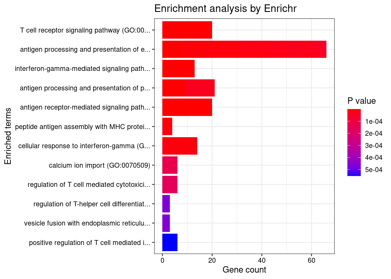
| Version | Author | Date |
|---|---|---|
| 4ded2ef | wesleycrouse | 2022-07-19 |
GO_Cellular_Component_2021
Term Overlap Adjusted.P.value Genes
1 MHC protein complex (GO:0042611) 12/20 9.080461e-12 HLA-DMA;HLA-DMB;HLA-B;HLA-C;HLA-DRA;HLA-F;HLA-DOA;HLA-DQA1;HLA-DQB2;HLA-DRB1;HLA-DPA1;HLA-DQB1
2 integral component of lumenal side of endoplasmic reticulum membrane (GO:0071556) 13/28 2.128437e-11 HLA-B;HLA-C;HLA-F;SPPL3;HLA-G;TAPBP;HLA-DRA;HLA-DQA2;HLA-DQA1;HLA-DQB2;HLA-DRB1;HLA-DPA1;HLA-DQB1
3 lumenal side of endoplasmic reticulum membrane (GO:0098553) 13/28 2.128437e-11 HLA-B;HLA-C;HLA-F;SPPL3;HLA-G;TAPBP;HLA-DRA;HLA-DQA2;HLA-DQA1;HLA-DQB2;HLA-DRB1;HLA-DPA1;HLA-DQB1
4 MHC class II protein complex (GO:0042613) 9/13 6.101987e-10 HLA-DMA;HLA-DMB;HLA-DRA;HLA-DOA;HLA-DQA1;HLA-DQB2;HLA-DRB1;HLA-DPA1;HLA-DQB1
5 integral component of endoplasmic reticulum membrane (GO:0030176) 19/142 1.733956e-06 ATF6B;TAP2;HLA-B;TAP1;HLA-C;ABCB9;ELOVL7;HLA-F;HLA-G;SPPL3;TAPBP;SPCS1;HLA-DRA;HLA-DQA2;HLA-DQA1;HLA-DRB1;HLA-DQB2;HLA-DPA1;HLA-DQB1
6 ER to Golgi transport vesicle membrane (GO:0012507) 11/54 1.454730e-05 HLA-B;HLA-C;HLA-DRA;HLA-F;HLA-G;HLA-DQA2;HLA-DQB2;HLA-DQA1;HLA-DRB1;HLA-DPA1;HLA-DQB1
7 COPII-coated ER to Golgi transport vesicle (GO:0030134) 13/79 1.454730e-05 HLA-B;DDHD2;HLA-C;HLA-F;HLA-G;HLA-DRA;HLA-DQA2;HLA-DQB2;HLA-DQA1;HLA-DRB1;TMED4;HLA-DPA1;HLA-DQB1
8 coated vesicle membrane (GO:0030662) 11/55 1.454730e-05 HLA-B;HLA-C;HLA-DRA;HLA-F;HLA-G;HLA-DQA2;HLA-DQB2;HLA-DQA1;HLA-DRB1;HLA-DPA1;HLA-DQB1
9 transport vesicle membrane (GO:0030658) 11/60 3.245875e-05 HLA-B;HLA-C;HLA-DRA;HLA-F;HLA-G;HLA-DQA2;HLA-DQB2;HLA-DQA1;HLA-DRB1;HLA-DPA1;HLA-DQB1
10 lytic vacuole membrane (GO:0098852) 21/267 9.908241e-04 SLC12A4;ABCB6;LRP1;ABCB9;HLA-F;CLCN3;RPTOR;HLA-DMA;HLA-DMB;GNB2;FLOT1;HLA-DRA;LAMTOR2;SLC39A8;HLA-DOA;HLA-DQA2;HLA-DQA1;HLA-DRB1;HLA-DQB2;HLA-DPA1;HLA-DQB1
11 lysosomal membrane (GO:0005765) 24/330 9.908241e-04 SLC12A4;ABCB6;LRP1;ABCB9;HLA-F;CLCN3;RPTOR;HLA-DMA;HLA-DMB;GNB2;SLCO4C1;TLR9;FLOT1;CDIP1;HLA-DRA;LAMTOR2;SLC39A8;HLA-DOA;HLA-DQA2;HLA-DQA1;HLA-DRB1;HLA-DQB2;HLA-DPA1;HLA-DQB1
12 Golgi membrane (GO:0000139) 30/472 1.258865e-03 B4GALT2;NOTCH4;FURIN;FUT2;GLG1;FUT9;MGAT3;HLA-DQA2;HLA-DQA1;ST3GAL3;HLA-DPA1;SREBF1;GALNT4;GALNT2;B3GAT1;B3GALT4;HLA-B;HLA-C;NOSIP;HLA-F;HLA-G;SREBF2;TAPBP;MGAT4C;TLR9;HLA-DRA;HLA-DRB1;HLA-DQB2;LLGL1;HLA-DQB1
13 endocytic vesicle membrane (GO:0030666) 15/158 1.258865e-03 LRP1;TAP2;HLA-B;TAP1;HLA-C;HLA-F;HLA-G;TAPBP;HLA-DRA;HLA-DQA2;HLA-DQA1;HLA-DRB1;HLA-DQB2;HLA-DPA1;HLA-DQB1
14 bounding membrane of organelle (GO:0098588) 42/767 1.368942e-03 B4GALT2;ABCB6;LRP1;NOTCH4;VPS4A;ATP2A2;FURIN;FUT2;CLCN3;SPPL3;GLG1;FUT9;MGAT3;DRD2;HLA-DQA2;HLA-DQA1;ST3GAL3;HLA-DPA1;SREBF1;GALNT4;GALNT2;B3GAT1;TAP2;B3GALT4;HLA-B;TAP1;HLA-C;NOSIP;VPS37A;HLA-F;HLA-G;SREBF2;TM6SF2;TAPBP;MGAT4C;NAT8;TLR9;HLA-DRA;LAMTOR2;HLA-DRB1;HLA-DQB2;HLA-DQB1
15 phagocytic vesicle (GO:0045335) 11/100 2.814581e-03 PDIA3;ZDHHC5;TAP2;HLA-B;TLR9;TAP1;HLA-C;HLA-F;CLCN3;HLA-G;TAPBP
16 phagocytic vesicle membrane (GO:0030670) 7/45 4.953534e-03 TAP2;HLA-B;HLA-C;TAP1;HLA-F;HLA-G;TAPBP
17 lysosome (GO:0005764) 26/477 2.786254e-02 ABCB6;LRP1;VPS4A;ABCB9;CLCN3;RPTOR;HLA-DMA;HLA-DMB;NEU1;FLOT1;SLC39A8;HLA-DOA;HLA-DQA2;HLA-DQA1;HLA-DPA1;SLC12A4;PRSS16;HLA-F;GNB2;TLR9;HLA-DRA;LAMTOR2;PPT2;HLA-DRB1;HLA-DQB2;HLA-DQB1
18 trans-Golgi network membrane (GO:0032588) 9/99 3.551826e-02 FUT9;HLA-DRA;HLA-DQA2;LLGL1;HLA-DQA1;HLA-DRB1;HLA-DQB2;HLA-DPA1;HLA-DQB1
19 endoplasmic reticulum-Golgi intermediate compartment membrane (GO:0033116) 6/49 4.022553e-02 NAT8;TAP2;TAP1;SPPL3;TAPBP;TM6SF2
20 endoplasmic reticulum membrane (GO:0005789) 34/712 4.607067e-02 NDRG4;ABCB6;ATF6B;NOTCH4;CISD2;ATP2A2;ABCB9;MOSPD3;AGPAT1;RNF5;CYP17A1;CYP2D6;HMOX2;SREBF1;GALNT2;ATP13A1;B3GAT1;TAP2;TAP1;ALG12;ELOVL7;VRK2;ATG13;SREBF2;TM6SF2;TAPBP;SPCS1;NAT8;TMX2;CYP21A2;LPCAT4;REEP2;TLR9;TKT
21 clathrin-coated endocytic vesicle membrane (GO:0030669) 7/69 4.924773e-02 HLA-DRA;HLA-DQA2;HLA-DQB2;HLA-DQA1;HLA-DRB1;HLA-DPA1;HLA-DQB1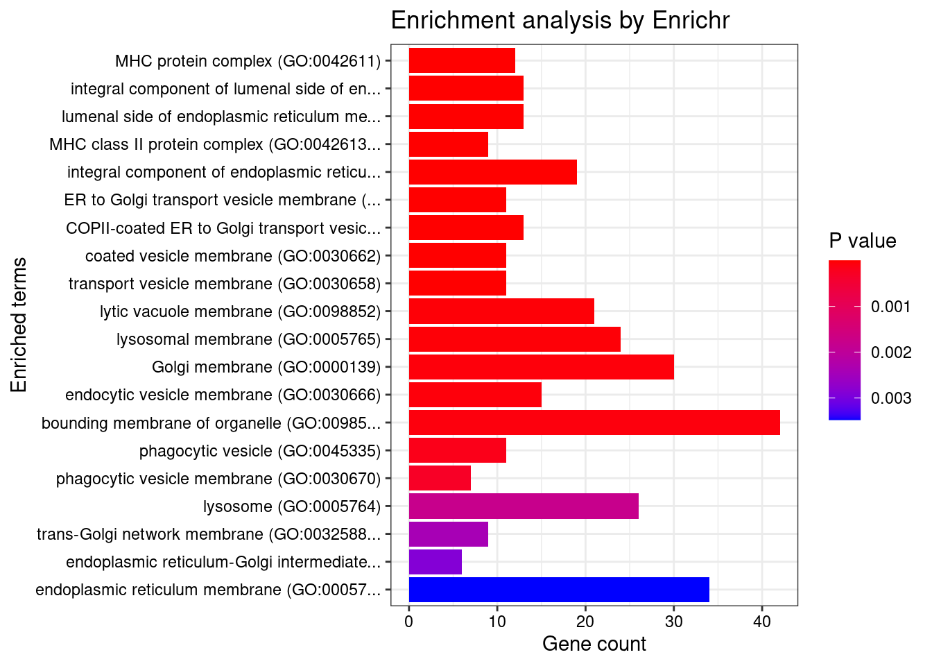
| Version | Author | Date |
|---|---|---|
| 4ded2ef | wesleycrouse | 2022-07-19 |
GO_Molecular_Function_2021
Term Overlap Adjusted.P.value Genes
1 MHC class II receptor activity (GO:0032395) 8/10 9.945111e-09 HLA-DRA;HLA-DOA;HLA-DQA2;HLA-DQA1;HLA-DQB2;HLA-DRB1;HLA-DPA1;HLA-DQB1
2 TAP1 binding (GO:0046978) 5/5 4.842754e-06 TAP2;TAP1;ABCB9;HLA-F;TAPBP
3 MHC class II protein complex binding (GO:0023026) 6/17 8.775342e-04 YWHAE;HLA-DMA;HLA-DMB;HLA-DRA;HLA-DOA;HLA-DRB1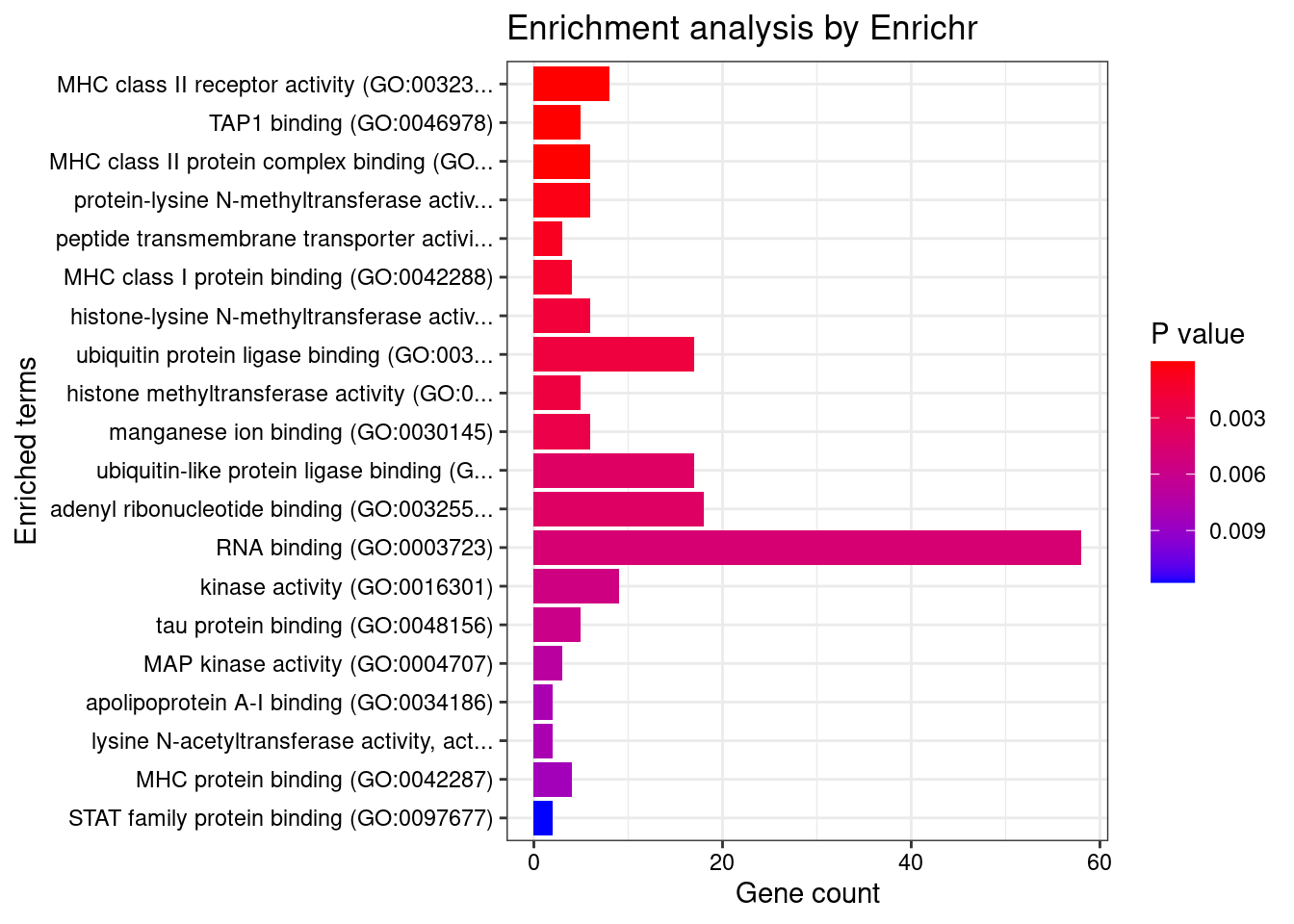
| Version | Author | Date |
|---|---|---|
| 4ded2ef | wesleycrouse | 2022-07-19 |
Enrichment analysis for cTWAS genes in top tissues separately
GO
output <- output[order(-output$pve_g),]
top_tissues <- output$weight[1:5]
for (tissue in top_tissues){
cat(paste0(tissue, "\n\n"))
ctwas_genes_tissue <- df[[tissue]]$ctwas
cat(paste0("Number of cTWAS Genes in Tissue: ", length(ctwas_genes_tissue), "\n\n"))
dbs <- c("GO_Biological_Process_2021")
GO_enrichment <- enrichr(ctwas_genes_tissue, dbs)
for (db in dbs){
cat(paste0("\n", db, "\n\n"))
enrich_results <- GO_enrichment[[db]]
enrich_results <- enrich_results[enrich_results$Adjusted.P.value<0.05,c("Term", "Overlap", "Adjusted.P.value", "Genes")]
print(enrich_results)
print(plotEnrich(GO_enrichment[[db]]))
}
}Artery_Aorta
Number of cTWAS Genes in Tissue: 12
Uploading data to Enrichr... Done.
Querying GO_Biological_Process_2021... Done.
Parsing results... Done.
GO_Biological_Process_2021
Term Overlap Adjusted.P.value Genes
1 positive regulation of neurogenesis (GO:0050769) 2/72 0.04008199 NGF;DRD2
2 modulation of chemical synaptic transmission (GO:0050804) 2/109 0.04008199 NGF;DRD2
3 defense response to symbiont (GO:0140546) 2/124 0.04008199 BNIP3L;IRF3
4 defense response to virus (GO:0051607) 2/133 0.04008199 BNIP3L;IRF3
5 regulation of catecholamine uptake involved in synaptic transmission (GO:0051940) 1/5 0.04008199 DRD2
6 response to cocaine (GO:0042220) 1/5 0.04008199 DRD2
7 response to morphine (GO:0043278) 1/5 0.04008199 DRD2
8 peristalsis (GO:0030432) 1/5 0.04008199 DRD2
9 neuron projection morphogenesis (GO:0048812) 2/140 0.04008199 NGF;DRD2
10 regulation of interleukin-1-mediated signaling pathway (GO:2000659) 1/6 0.04008199 VRK2
11 negative regulation of cytosolic calcium ion concentration (GO:0051481) 1/6 0.04008199 DRD2
12 tRNA 3'-end processing (GO:0042780) 1/6 0.04008199 ELAC2
13 mitochondrial protein catabolic process (GO:0035694) 1/6 0.04008199 BNIP3L
14 positive regulation of growth hormone secretion (GO:0060124) 1/6 0.04008199 DRD2
15 prepulse inhibition (GO:0060134) 1/6 0.04008199 DRD2
16 negative regulation of cellular process (GO:0048523) 3/566 0.04008199 BNIP3L;NGF;DRD2
17 regulation of growth hormone secretion (GO:0060123) 1/7 0.04008199 DRD2
18 response to alkaloid (GO:0043279) 1/7 0.04008199 DRD2
19 phospholipase C-activating dopamine receptor signaling pathway (GO:0060158) 1/7 0.04008199 DRD2
20 mitochondrial RNA processing (GO:0000963) 1/8 0.04008199 ELAC2
21 mitochondrial tRNA processing (GO:0090646) 1/8 0.04008199 ELAC2
22 regulation of collateral sprouting (GO:0048670) 1/8 0.04008199 NGF
23 regulation of dopamine receptor signaling pathway (GO:0060159) 1/8 0.04008199 DRD2
24 regulation of dopamine uptake involved in synaptic transmission (GO:0051584) 1/8 0.04008199 DRD2
25 associative learning (GO:0008306) 1/9 0.04008199 DRD2
26 positive regulation of mitochondrial membrane permeability involved in apoptotic process (GO:1902110) 1/9 0.04008199 BNIP3L
27 regulation of programmed cell death (GO:0043067) 2/194 0.04008199 BNIP3L;IRF3
28 negative regulation of voltage-gated calcium channel activity (GO:1901386) 1/10 0.04008199 DRD2
29 nerve growth factor signaling pathway (GO:0038180) 1/10 0.04008199 NGF
30 arachidonate transport (GO:1903963) 1/10 0.04008199 DRD2
31 arachidonic acid secretion (GO:0050482) 1/10 0.04008199 DRD2
32 cytoplasmic pattern recognition receptor signaling pathway in response to virus (GO:0039528) 1/10 0.04008199 IRF3
33 response to histamine (GO:0034776) 1/10 0.04008199 DRD2
34 positive regulation of neuroblast proliferation (GO:0002052) 1/11 0.04040492 DRD2
35 regulation of long-term neuronal synaptic plasticity (GO:0048169) 1/11 0.04040492 DRD2
36 protein kinase C-activating G protein-coupled receptor signaling pathway (GO:0007205) 1/11 0.04040492 PRKD3
37 phasic smooth muscle contraction (GO:0014821) 1/12 0.04287502 DRD2
38 mitochondrial outer membrane permeabilization (GO:0097345) 1/13 0.04295255 BNIP3L
39 icosanoid secretion (GO:0032309) 1/13 0.04295255 DRD2
40 negative regulation of adenylate cyclase activity (GO:0007194) 1/13 0.04295255 DRD2
41 negative regulation of cyclase activity (GO:0031280) 1/14 0.04307255 DRD2
42 regulation of apoptotic process (GO:0042981) 3/742 0.04307255 BNIP3L;IRF3;NGF
43 negative regulation of blood pressure (GO:0045776) 1/15 0.04307255 DRD2
44 regulation of synaptic transmission, GABAergic (GO:0032228) 1/15 0.04307255 DRD2
45 neurotrophin TRK receptor signaling pathway (GO:0048011) 1/15 0.04307255 NGF
46 catecholamine metabolic process (GO:0006584) 1/15 0.04307255 DRD2
47 RNA splicing, via transesterification reactions with bulged adenosine as nucleophile (GO:0000377) 2/251 0.04311931 CWC25;SF3B1
48 regulation of systemic arterial blood pressure (GO:0003073) 1/16 0.04311931 DRD2
49 negative regulation of lyase activity (GO:0051350) 1/16 0.04311931 DRD2
50 adenylate cyclase-activating adrenergic receptor signaling pathway (GO:0071880) 1/17 0.04400555 DRD2
51 regulation of neuroblast proliferation (GO:1902692) 1/17 0.04400555 DRD2
52 mRNA splicing, via spliceosome (GO:0000398) 2/274 0.04511199 CWC25;SF3B1
53 excitatory postsynaptic potential (GO:0060079) 1/19 0.04511199 DRD2
54 dopamine metabolic process (GO:0042417) 1/19 0.04511199 DRD2
55 adrenergic receptor signaling pathway (GO:0071875) 1/20 0.04511199 DRD2
56 positive regulation of interferon-alpha production (GO:0032727) 1/20 0.04511199 IRF3
57 positive regulation of programmed cell death (GO:0043068) 2/286 0.04511199 BNIP3L;NGF
58 neurotrophin signaling pathway (GO:0038179) 1/21 0.04511199 NGF
59 positive regulation of neural precursor cell proliferation (GO:2000179) 1/22 0.04511199 DRD2
60 cellular response to nerve growth factor stimulus (GO:1990090) 1/22 0.04511199 NGF
61 regulation of adenylate cyclase activity (GO:0045761) 1/22 0.04511199 DRD2
62 regulation of voltage-gated calcium channel activity (GO:1901385) 1/22 0.04511199 DRD2
63 mRNA processing (GO:0006397) 2/300 0.04511199 CWC25;SF3B1
64 regulation of cysteine-type endopeptidase activity (GO:2000116) 1/23 0.04511199 NGF
65 positive regulation of apoptotic process (GO:0043065) 2/310 0.04511199 BNIP3L;NGF
66 negative regulation of synaptic transmission (GO:0050805) 1/24 0.04511199 DRD2
67 ncRNA 3'-end processing (GO:0043628) 1/24 0.04511199 ELAC2
68 negative regulation of sequestering of calcium ion (GO:0051283) 1/25 0.04511199 DRD2
69 regulation of interferon-alpha production (GO:0032647) 1/25 0.04511199 IRF3
70 chemical synaptic transmission, postsynaptic (GO:0099565) 1/25 0.04511199 DRD2
71 peripheral nervous system development (GO:0007422) 1/25 0.04511199 NGF
72 regulation of dopamine secretion (GO:0014059) 1/25 0.04511199 DRD2
73 RNA splicing, via transesterification reactions (GO:0000375) 1/25 0.04511199 SF3B1
74 negative regulation of protein transport (GO:0051224) 1/26 0.04626976 DRD2
75 negative regulation of cation channel activity (GO:2001258) 1/27 0.04664962 DRD2
76 release of sequestered calcium ion into cytosol (GO:0051209) 1/27 0.04664962 DRD2
77 positive regulation of cytokine production (GO:0001819) 2/335 0.04664962 IRF3;DRD2
78 negative regulation of calcium ion transmembrane transporter activity (GO:1901020) 1/28 0.04664962 DRD2
79 positive regulation of cytosolic calcium ion concentration involved in phospholipase C-activating G protein-coupled signaling pathway (GO:0051482) 1/28 0.04664962 DRD2
80 regulation of neuronal synaptic plasticity (GO:0048168) 1/29 0.04698083 DRD2
81 extrinsic apoptotic signaling pathway via death domain receptors (GO:0008625) 1/30 0.04698083 NGF
82 positive regulation of small GTPase mediated signal transduction (GO:0051057) 1/30 0.04698083 NGF
83 TRIF-dependent toll-like receptor signaling pathway (GO:0035666) 1/30 0.04698083 IRF3
84 regulation of catecholamine secretion (GO:0050433) 1/30 0.04698083 DRD2
85 MyD88-independent toll-like receptor signaling pathway (GO:0002756) 1/31 0.04740485 IRF3
86 regulation of potassium ion transport (GO:0043266) 1/31 0.04740485 DRD2
| Version | Author | Date |
|---|---|---|
| 4ded2ef | wesleycrouse | 2022-07-19 |
Brain_Hypothalamus
Number of cTWAS Genes in Tissue: 17
Uploading data to Enrichr... Done.
Querying GO_Biological_Process_2021... Done.
Parsing results... Done.
GO_Biological_Process_2021

[1] Term             Overlap          Adjusted.P.value Genes
<0 rows> (or 0-length row.names)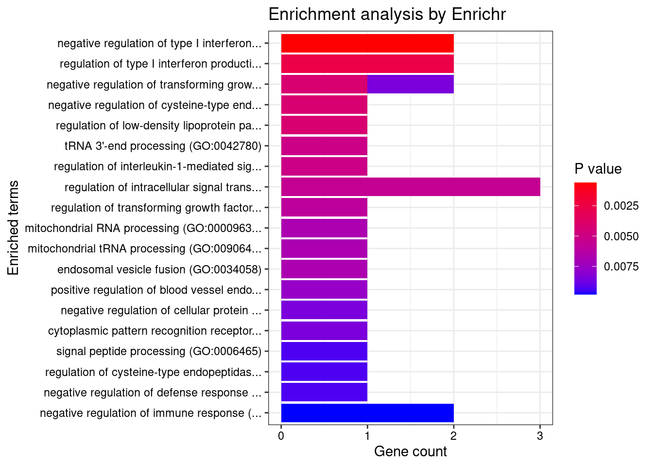
| Version | Author | Date |
|---|---|---|
| 4ded2ef | wesleycrouse | 2022-07-19 |
Heart_Atrial_Appendage
Number of cTWAS Genes in Tissue: 7
Uploading data to Enrichr... Done.
Querying GO_Biological_Process_2021... Done.
Parsing results... Done.
GO_Biological_Process_2021
Term Overlap Adjusted.P.value Genes
1 tRNA 3'-end processing (GO:0042780) 1/6 0.03020776 ELAC2
2 regulation of mesenchymal stem cell differentiation (GO:2000739) 1/7 0.03020776 SOX5
3 chromatin silencing at telomere (GO:0006348) 1/8 0.03020776 DOT1L
4 mitochondrial RNA processing (GO:0000963) 1/8 0.03020776 ELAC2
5 mitochondrial tRNA processing (GO:0090646) 1/8 0.03020776 ELAC2
6 positive regulation of chondrocyte differentiation (GO:0032332) 1/11 0.03393294 SOX5
7 regulation of receptor signaling pathway via STAT (GO:1904892) 1/13 0.03393294 DOT1L
8 positive regulation of stem cell differentiation (GO:2000738) 1/17 0.03393294 SOX5
9 regulation of cartilage development (GO:0061035) 1/18 0.03393294 SOX5
10 positive regulation of cartilage development (GO:0061036) 1/18 0.03393294 SOX5
11 ncRNA 3'-end processing (GO:0043628) 1/24 0.03630775 ELAC2
12 RNA splicing, via transesterification reactions (GO:0000375) 1/25 0.03630775 SF3B1
13 regulation of chondrocyte differentiation (GO:0032330) 1/26 0.03630775 SOX5
14 regulation of transcription regulatory region DNA binding (GO:2000677) 1/27 0.03630775 DOT1L
15 chondrocyte differentiation (GO:0002062) 1/32 0.03761302 SOX5
16 DNA damage checkpoint signaling (GO:0000077) 1/32 0.03761302 DOT1L
17 histone lysine methylation (GO:0034968) 1/34 0.03761302 DOT1L
18 connective tissue development (GO:0061448) 1/38 0.03835591 SOX5
19 DNA integrity checkpoint signaling (GO:0031570) 1/39 0.03835591 DOT1L
20 regulation of receptor signaling pathway via JAK-STAT (GO:0046425) 1/45 0.03835591 DOT1L
21 spliceosomal complex assembly (GO:0000245) 1/46 0.03835591 SF3B1
22 regulation of DNA binding (GO:0051101) 1/47 0.03835591 DOT1L
23 telomere organization (GO:0032200) 1/47 0.03835591 DOT1L
24 cartilage development (GO:0051216) 1/52 0.03901219 SOX5
25 signal transduction in response to DNA damage (GO:0042770) 1/52 0.03901219 DOT1L
26 positive regulation of gene expression, epigenetic (GO:0045815) 1/57 0.04108783 SF3B1
27 tRNA processing (GO:0008033) 1/64 0.04437848 ELAC2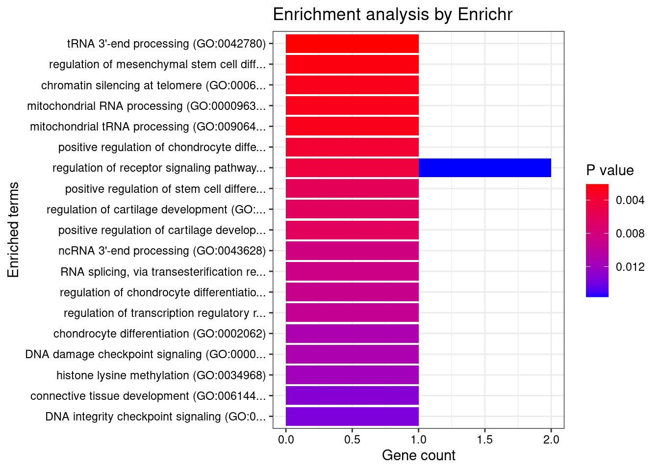
| Version | Author | Date |
|---|---|---|
| 4ded2ef | wesleycrouse | 2022-07-19 |
Esophagus_Gastroesophageal_Junction
Number of cTWAS Genes in Tissue: 9
Uploading data to Enrichr... Done.
Querying GO_Biological_Process_2021... Done.
Parsing results... Done.
GO_Biological_Process_2021
Term Overlap Adjusted.P.value Genes
1 tRNA 3'-end processing (GO:0042780) 1/6 0.04959140 ELAC2
2 mitochondrial RNA processing (GO:0000963) 1/8 0.04959140 ELAC2
3 mitochondrial tRNA processing (GO:0090646) 1/8 0.04959140 ELAC2
4 negative regulation of transcription by competitive promoter binding (GO:0010944) 1/10 0.04959140 BHLHE41
5 negative regulation of myotube differentiation (GO:0010832) 1/13 0.04959140 BHLHE41
6 actin filament capping (GO:0051693) 1/19 0.04959140 SVIL
7 negative regulation of striated muscle cell differentiation (GO:0051154) 1/19 0.04959140 BHLHE41
8 barbed-end actin filament capping (GO:0051016) 1/19 0.04959140 SVIL
9 ncRNA 3'-end processing (GO:0043628) 1/24 0.04959140 ELAC2
10 regulation of myotube differentiation (GO:0010830) 1/25 0.04959140 BHLHE41
11 RNA splicing, via transesterification reactions (GO:0000375) 1/25 0.04959140 SF3B1
12 skeletal muscle organ development (GO:0060538) 1/32 0.04959140 SVIL
13 actin filament bundle assembly (GO:0051017) 1/33 0.04959140 CALD1
14 actin filament bundle organization (GO:0061572) 1/33 0.04959140 CALD1
15 striated muscle tissue development (GO:0014706) 1/34 0.04959140 SVIL
16 skeletal muscle tissue development (GO:0007519) 1/37 0.04959140 SVIL
17 positive regulation of cytokinesis (GO:0032467) 1/37 0.04959140 SVIL
18 regulation of cell development (GO:0060284) 1/41 0.04982091 BHLHE41
19 regulation of nervous system development (GO:0051960) 1/42 0.04982091 BHLHE41
20 positive regulation of cell division (GO:0051781) 1/44 0.04982091 SVIL
21 spliceosomal complex assembly (GO:0000245) 1/46 0.04982091 SF3B1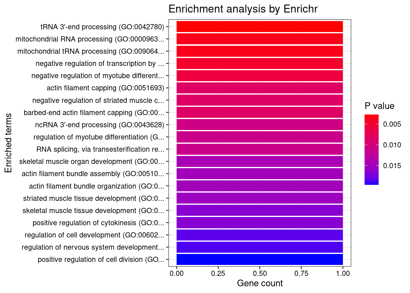
| Version | Author | Date |
|---|---|---|
| 4ded2ef | wesleycrouse | 2022-07-19 |
Whole_Blood
Number of cTWAS Genes in Tissue: 6
Uploading data to Enrichr... Done.
Querying GO_Biological_Process_2021... Done.
Parsing results... Done.
GO_Biological_Process_2021
Term Overlap Adjusted.P.value Genes
1 tRNA 3'-end processing (GO:0042780) 1/6 0.01438715 ELAC2
2 mitochondrial tRNA processing (GO:0090646) 1/8 0.01438715 ELAC2
3 mitochondrial RNA processing (GO:0000963) 1/8 0.01438715 ELAC2
4 ncRNA 3'-end processing (GO:0043628) 1/24 0.02691881 ELAC2
5 RNA splicing, via transesterification reactions (GO:0000375) 1/25 0.02691881 SF3B1
6 spliceosomal complex assembly (GO:0000245) 1/46 0.04116743 SF3B1
7 positive regulation of gene expression, epigenetic (GO:0045815) 1/57 0.04286085 SF3B1
8 tRNA processing (GO:0008033) 1/64 0.04286085 ELAC2
9 regulation of gene expression, epigenetic (GO:0040029) 1/82 0.04870414 SF3B1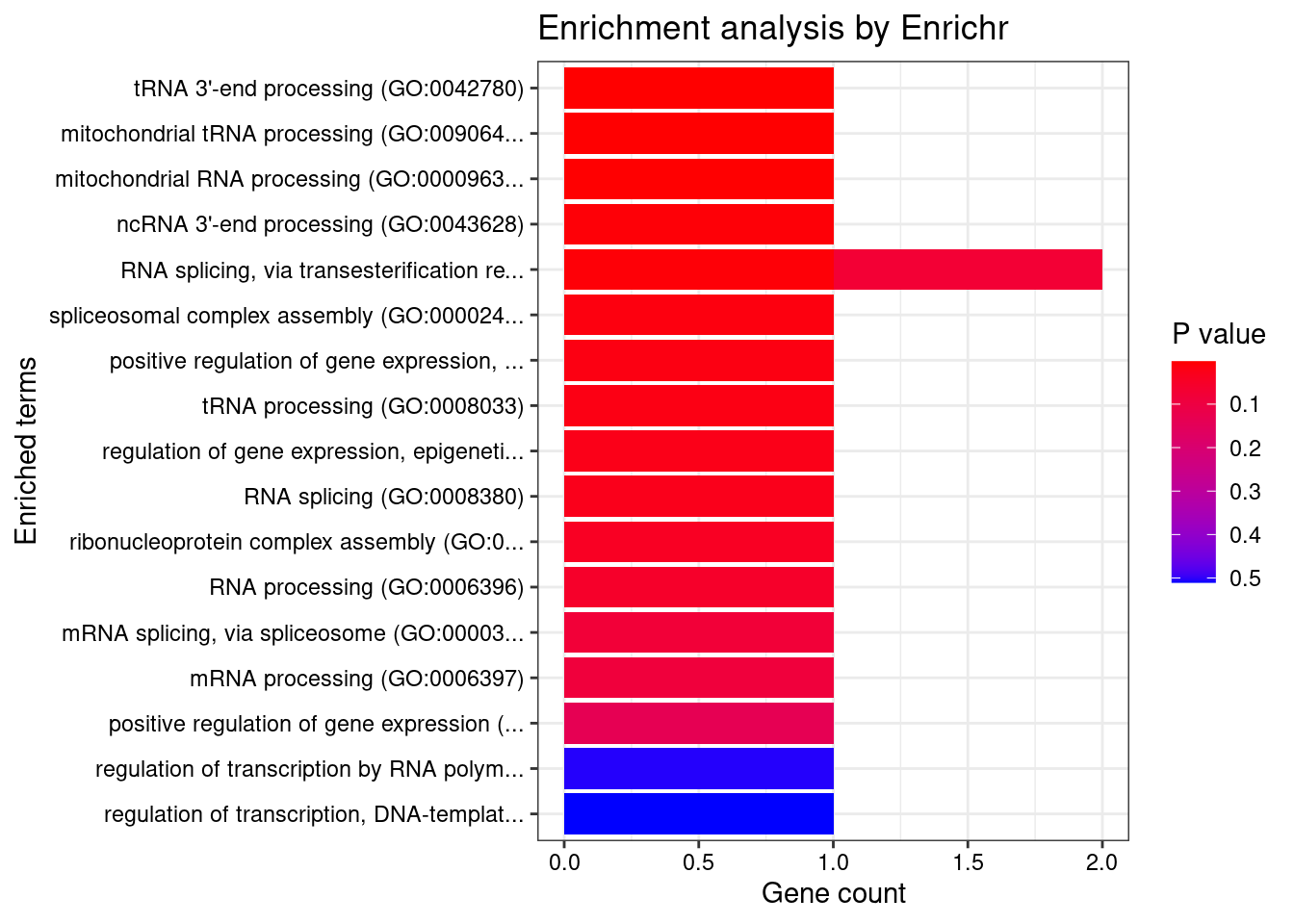
| Version | Author | Date |
|---|---|---|
| 4ded2ef | wesleycrouse | 2022-07-19 |
KEGG
output <- output[order(-output$pve_g),]
top_tissues <- output$weight[1:5]
for (tissue in top_tissues){
cat(paste0(tissue, "\n\n"))
ctwas_genes_tissue <- df[[tissue]]$ctwas
background_tissue <- df[[tissue]]$gene_pips$genename
cat(paste0("Number of cTWAS Genes in Tissue: ", length(ctwas_genes_tissue), "\n\n"))
databases <- c("pathway_KEGG")
enrichResult <- NULL
try(enrichResult <- WebGestaltR(enrichMethod="ORA", organism="hsapiens",
interestGene=ctwas_genes_tissue, referenceGene=background_tissue,
enrichDatabase=databases, interestGeneType="genesymbol",
referenceGeneType="genesymbol", isOutput=F))
if (!is.null(enrichResult)){
print(enrichResult[,c("description", "size", "overlap", "FDR", "userId")])
}
cat("\n")
} Artery_Aorta
Number of cTWAS Genes in Tissue: 12
Loading the functional categories...
Loading the ID list...
Loading the reference list...
Performing the enrichment analysis...
Warning in oraEnrichment(interestGeneList, referenceGeneList, geneSet, minNum = minNum, : No significant gene set is identified based on FDR 0.05!
Brain_Hypothalamus

Number of cTWAS Genes in Tissue: 17

Loading the functional categories...
Loading the ID list...
Loading the reference list...
Performing the enrichment analysis...
Warning in oraEnrichment(interestGeneList, referenceGeneList, geneSet, minNum = minNum, : No significant gene set is identified based on FDR 0.05!
Heart_Atrial_Appendage

Number of cTWAS Genes in Tissue: 7

Loading the functional categories...
Loading the ID list...
Loading the reference list...
Performing the enrichment analysis...
Warning in oraEnrichment(interestGeneList, referenceGeneList, geneSet, minNum = minNum, : No significant gene set is identified based on FDR 0.05!
Esophagus_Gastroesophageal_Junction

Number of cTWAS Genes in Tissue: 9

Loading the functional categories...
Loading the ID list...
Loading the reference list...
Performing the enrichment analysis...
Warning in oraEnrichment(interestGeneList, referenceGeneList, geneSet, minNum = minNum, : No significant gene set is identified based on FDR 0.05!
Whole_Blood

Number of cTWAS Genes in Tissue: 6

Loading the functional categories...
Loading the ID list...
Loading the reference list...
Performing the enrichment analysis...
Warning in oraEnrichment(interestGeneList, referenceGeneList, geneSet, minNum = minNum, : No significant gene set is identified based on FDR 0.05!DisGeNET
output <- output[order(-output$pve_g),]
top_tissues <- output$weight[1:5]

for (tissue in top_tissues){
  cat(paste0(tissue, "\n\n"))

  ctwas_genes_tissue <- df[[tissue]]$ctwas

  cat(paste0("Number of cTWAS Genes in Tissue: ", length(ctwas_genes_tissue), "\n\n"))

  res_enrich <- disease_enrichment(entities=ctwas_genes_tissue, vocabulary = "HGNC", database = "CURATED")

  if (any(res_enrich@qresult$FDR < 0.05)){
    print(res_enrich@qresult[res_enrich@qresult$FDR < 0.05, c("Description", "FDR", "Ratio",  "BgRatio")])
  }

  cat("\n")
}
Gene sets curated by Macarthur Lab
output <- output[order(-output$pve_g),]
top_tissues <- output$weight[1:5]

gene_set_dir <- "/project2/mstephens/wcrouse/gene_sets/"
gene_set_files <- c("gwascatalog.tsv",
                    "mgi_essential.tsv",
                    "core_essentials_hart.tsv",
                    "clinvar_path_likelypath.tsv",
                    "fda_approved_drug_targets.tsv")

for (tissue in top_tissues){
  cat(paste0(tissue, "\n\n"))

  ctwas_genes_tissue <- df[[tissue]]$ctwas
  background_tissue <- df[[tissue]]$gene_pips$genename

  cat(paste0("Number of cTWAS Genes in Tissue: ", length(ctwas_genes_tissue), "\n\n"))

  gene_sets <- lapply(gene_set_files, function(x){as.character(read.table(paste0(gene_set_dir, x))[,1])})
  names(gene_sets) <- sapply(gene_set_files, function(x){unlist(strsplit(x, "[.]"))[1]})

  gene_lists <- list(ctwas_genes_tissue=ctwas_genes_tissue)

  #genes in gene_sets filtered to ensure inclusion in background
  gene_sets <- lapply(gene_sets, function(x){x[x %in% background_tissue]})

  ##########
  hyp_score <- data.frame()
  size <- c()
  ngenes <- c()

  for (i in 1:length(gene_sets)) {
    for (j in 1:length(gene_lists)){
      group1 <- length(gene_sets[[i]])
      group2 <- length(as.vector(gene_lists[[j]]))
      size <- c(size, group1)
      Overlap <- length(intersect(gene_sets[[i]],as.vector(gene_lists[[j]])))
      ngenes <- c(ngenes, Overlap)
      Total <- length(background_tissue)
      hyp_score[i,j] <- phyper(Overlap-1, group2, Total-group2, group1,lower.tail=F)
    }
  }
  rownames(hyp_score) <- names(gene_sets)
  colnames(hyp_score) <- names(gene_lists)

  hyp_score_padj <- apply(hyp_score,2, p.adjust, method="BH", n=(nrow(hyp_score)*ncol(hyp_score)))
  hyp_score_padj <- as.data.frame(hyp_score_padj)
  hyp_score_padj$gene_set <- rownames(hyp_score_padj)
  hyp_score_padj$nset <- size
  hyp_score_padj$ngenes <- ngenes
  hyp_score_padj$percent <- ngenes/size

  hyp_score_padj <- hyp_score_padj[order(hyp_score_padj$ctwas_genes),]
  colnames(hyp_score_padj)[1] <- "padj"
  hyp_score_padj <- hyp_score_padj[,c(2:5,1)]
  rownames(hyp_score_padj)<- NULL

  print(hyp_score_padj)

  cat("\n")
}
Artery_Aorta
Number of cTWAS Genes in Tissue: 12
gene_set nset ngenes percent padj
1 gwascatalog 3448 10 0.002900232 0.004823331
2 core_essentials_hart 161 1 0.006211180 0.250380038
3 clinvar_path_likelypath 1609 4 0.002486016 0.250380038
4 fda_approved_drug_targets 179 1 0.005586592 0.250380038
5 mgi_essential 1247 2 0.001603849 0.468446049
Brain_Hypothalamus
Number of cTWAS Genes in Tissue: 17
gene_set nset ngenes percent padj
1 gwascatalog 2951 10 0.003388682 0.1918764
2 core_essentials_hart 137 1 0.007299270 0.6086098
3 mgi_essential 1015 2 0.001970443 0.9917306
4 clinvar_path_likelypath 1380 2 0.001449275 0.9917306
5 fda_approved_drug_targets 155 0 0.000000000 1.0000000
Heart_Atrial_Appendage
Number of cTWAS Genes in Tissue: 7
gene_set nset ngenes percent padj
1 gwascatalog 3331 7 0.0021014710 0.003808569
2 mgi_essential 1193 3 0.0025146689 0.124159501
3 core_essentials_hart 163 1 0.0061349693 0.194393800
4 clinvar_path_likelypath 1527 1 0.0006548788 0.894784712
5 fda_approved_drug_targets 165 0 0.0000000000 1.000000000
Esophagus_Gastroesophageal_Junction
Number of cTWAS Genes in Tissue: 9
gene_set nset ngenes percent padj
1 gwascatalog 3366 6 0.001782531 0.3037832
2 core_essentials_hart 152 1 0.006578947 0.3425965
3 mgi_essential 1181 2 0.001693480 0.5280701
4 clinvar_path_likelypath 1529 2 0.001308044 0.5576797
5 fda_approved_drug_targets 170 0 0.000000000 1.0000000
Whole_Blood
Number of cTWAS Genes in Tissue: 6
gene_set nset ngenes percent padj
1 gwascatalog 3119 5 0.0016030779 0.1246471
2 core_essentials_hart 148 1 0.0067567568 0.2447384
3 mgi_essential 1118 1 0.0008944544 0.8300178
4 clinvar_path_likelypath 1445 1 0.0006920415 0.8300178
5 fda_approved_drug_targets 152 0 0.0000000000 1.0000000Summary of results across tissues
weight_groups <- as.data.frame(matrix(c("Adipose_Subcutaneous", "Adipose",
                                        "Adipose_Visceral_Omentum", "Adipose",
                                        "Adrenal_Gland", "Endocrine",
                                        "Artery_Aorta", "Cardiovascular",
                                        "Artery_Coronary", "Cardiovascular",
                                        "Artery_Tibial", "Cardiovascular",
                                        "Brain_Amygdala", "CNS",
                                        "Brain_Anterior_cingulate_cortex_BA24", "CNS",
                                        "Brain_Caudate_basal_ganglia", "CNS",
                                        "Brain_Cerebellar_Hemisphere", "CNS",
                                        "Brain_Cerebellum", "CNS",
                                        "Brain_Cortex", "CNS",
                                        "Brain_Frontal_Cortex_BA9", "CNS",
                                        "Brain_Hippocampus", "CNS",
                                        "Brain_Hypothalamus", "CNS",
                                        "Brain_Nucleus_accumbens_basal_ganglia", "CNS",
                                        "Brain_Putamen_basal_ganglia", "CNS",
                                        "Brain_Spinal_cord_cervical_c-1", "CNS",
                                        "Brain_Substantia_nigra", "CNS",
                                        "Breast_Mammary_Tissue", "None",
                                        "Cells_Cultured_fibroblasts", "Skin",
                                        "Cells_EBV-transformed_lymphocytes", "Blood or Immune",
                                        "Colon_Sigmoid", "Digestive",
                                        "Colon_Transverse", "Digestive",
                                        "Esophagus_Gastroesophageal_Junction", "Digestive",
                                        "Esophagus_Mucosa", "Digestive",
                                        "Esophagus_Muscularis", "Digestive",
                                        "Heart_Atrial_Appendage", "Cardiovascular",
                                        "Heart_Left_Ventricle", "Cardiovascular",
                                        "Kidney_Cortex", "None",
                                        "Liver", "None",
                                        "Lung", "None",
                                        "Minor_Salivary_Gland", "None",
                                        "Muscle_Skeletal", "None",
                                        "Nerve_Tibial", "None",
                                        "Ovary", "None",
                                        "Pancreas", "None",
                                        "Pituitary", "Endocrine",
                                        "Prostate", "None",
                                        "Skin_Not_Sun_Exposed_Suprapubic", "Skin",
                                        "Skin_Sun_Exposed_Lower_leg", "Skin",
                                        "Small_Intestine_Terminal_Ileum", "Digestive",
                                        "Spleen", "Blood or Immune",
                                        "Stomach", "Digestive",
                                        "Testis", "Endocrine",
                                        "Thyroid", "Endocrine",
                                        "Uterus", "None",
                                        "Vagina", "None",
                                        "Whole_Blood", "Blood or Immune"),
                                      nrow=49, ncol=2, byrow=T), stringsAsFactors=F)
colnames(weight_groups) <- c("weight", "group")

#display tissue groups
print(weight_groups)
weight group
1 Adipose_Subcutaneous Adipose
2 Adipose_Visceral_Omentum Adipose
3 Adrenal_Gland Endocrine
4 Artery_Aorta Cardiovascular
5 Artery_Coronary Cardiovascular
6 Artery_Tibial Cardiovascular
7 Brain_Amygdala CNS
8 Brain_Anterior_cingulate_cortex_BA24 CNS
9 Brain_Caudate_basal_ganglia CNS
10 Brain_Cerebellar_Hemisphere CNS
11 Brain_Cerebellum CNS
12 Brain_Cortex CNS
13 Brain_Frontal_Cortex_BA9 CNS
14 Brain_Hippocampus CNS
15 Brain_Hypothalamus CNS
16 Brain_Nucleus_accumbens_basal_ganglia CNS
17 Brain_Putamen_basal_ganglia CNS
18 Brain_Spinal_cord_cervical_c-1 CNS
19 Brain_Substantia_nigra CNS
20 Breast_Mammary_Tissue None
21 Cells_Cultured_fibroblasts Skin
22 Cells_EBV-transformed_lymphocytes Blood or Immune
23 Colon_Sigmoid Digestive
24 Colon_Transverse Digestive
25 Esophagus_Gastroesophageal_Junction Digestive
26 Esophagus_Mucosa Digestive
27 Esophagus_Muscularis Digestive
28 Heart_Atrial_Appendage Cardiovascular
29 Heart_Left_Ventricle Cardiovascular
30 Kidney_Cortex None
31 Liver None
32 Lung None
33 Minor_Salivary_Gland None
34 Muscle_Skeletal None
35 Nerve_Tibial None
36 Ovary None
37 Pancreas None
38 Pituitary Endocrine
39 Prostate None
40 Skin_Not_Sun_Exposed_Suprapubic Skin
41 Skin_Sun_Exposed_Lower_leg Skin
42 Small_Intestine_Terminal_Ileum Digestive
43 Spleen Blood or Immune
44 Stomach Digestive
45 Testis Endocrine
46 Thyroid Endocrine
47 Uterus None
48 Vagina None
49 Whole_Blood Blood or Immunegroups <- unique(weight_groups$group)
df_group <- list()
for (i in 1:length(groups)){
group <- groups[i]
weights <- weight_groups$weight[weight_groups$group==group]
df_group[[group]] <- list(ctwas=unique(unlist(lapply(df[weights], function(x){x$ctwas}))),
background=unique(unlist(lapply(df[weights], function(x){x$gene_pips$genename}))))
}
output <- output[sapply(weight_groups$weight, match, output$weight),,drop=F]
output$group <- weight_groups$group
output$n_ctwas_group <- sapply(output$group, function(x){length(df_group[[x]][["ctwas"]])})
output$n_ctwas_group[output$group=="None"] <- 0
#barplot of number of cTWAS genes in each tissue
output <- output[order(-output$n_ctwas),,drop=F]
par(mar=c(10.1, 4.1, 4.1, 2.1))
barplot(output$n_ctwas, names.arg=output$weight, las=2, ylab="Number of cTWAS Genes", cex.names=0.6, main="Number of cTWAS Genes by Tissue")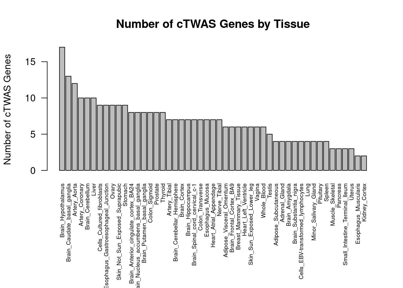
| Version | Author | Date |
|---|---|---|
| 4ded2ef | wesleycrouse | 2022-07-19 |
#barplot of number of cTWAS genes in each tissue
df_plot <- -sort(-sapply(groups[groups!="None"], function(x){length(df_group[[x]][["ctwas"]])}))

par(mar=c(10.1, 4.1, 4.1, 2.1))
barplot(df_plot, las=2, ylab="Number of cTWAS Genes", main="Number of cTWAS Genes by Tissue Group")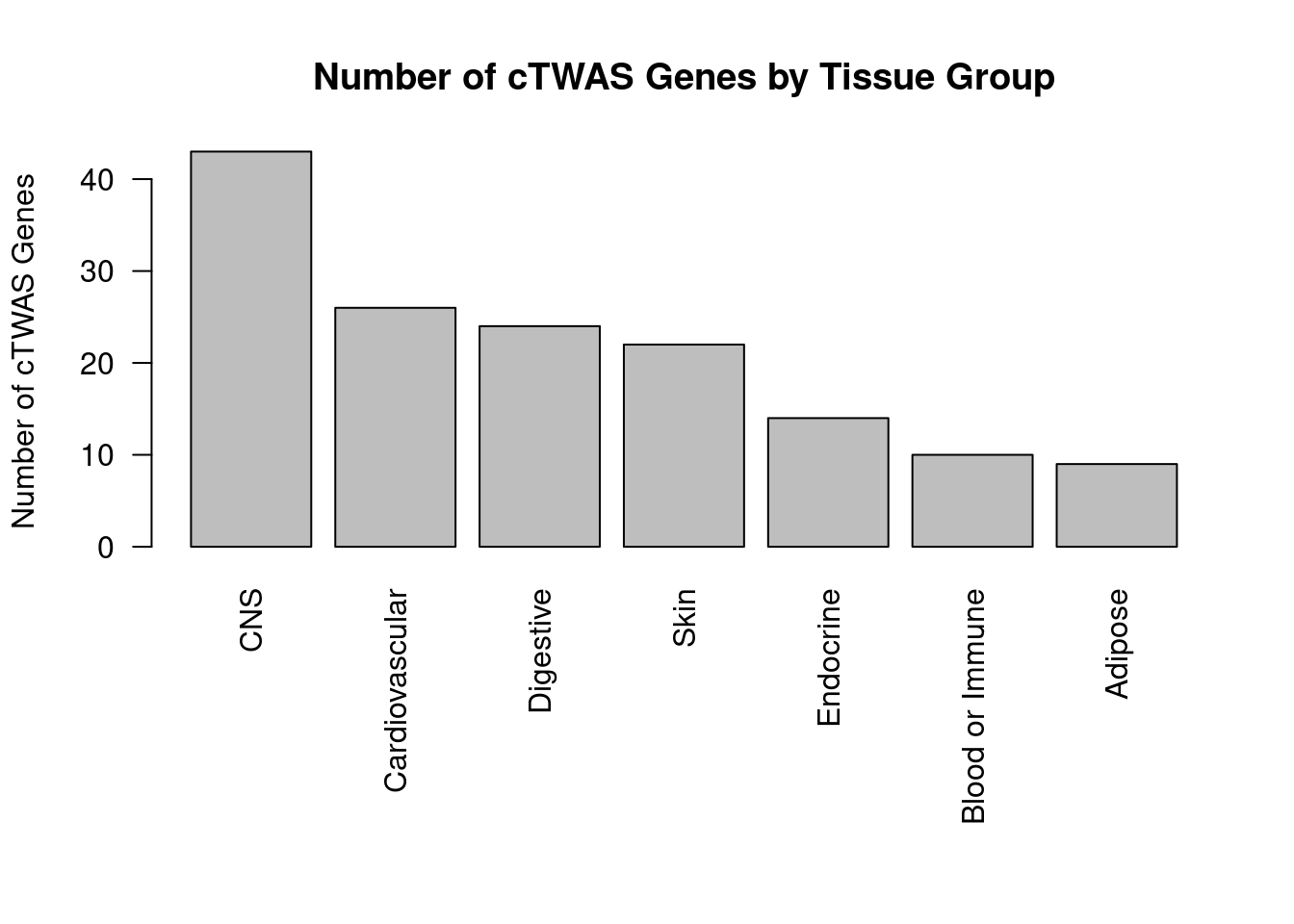
| Version | Author | Date |
|---|---|---|
| 4ded2ef | wesleycrouse | 2022-07-19 |
Enrichment analysis for cTWAS genes in each tissue group
GO
suppressWarnings(rm(group_enrichment_results))

for (group in names(df_group)){
  cat(paste0(group, "\n\n"))

  ctwas_genes_group <- df_group[[group]]$ctwas

  cat(paste0("Number of cTWAS Genes in Tissue Group: ", length(ctwas_genes_group), "\n\n"))

  dbs <- c("GO_Biological_Process_2021")
  GO_enrichment <- enrichr(ctwas_genes_group, dbs)

  for (db in dbs){
    cat(paste0("\n", db, "\n\n"))
    enrich_results <- GO_enrichment[[db]]
    enrich_results <- enrich_results[enrich_results$Adjusted.P.value<0.05,c("Term", "Overlap", "Adjusted.P.value", "Genes")]
    print(enrich_results)
    print(plotEnrich(GO_enrichment[[db]]))

    if (nrow(enrich_results)>0){
      if (!exists("group_enrichment_results")){
        group_enrichment_results <- cbind(group, db, enrich_results)
      } else {
        group_enrichment_results <- rbind(group_enrichment_results, cbind(group, db, enrich_results))
      }
    }
  }

}
Adipose
Number of cTWAS Genes in Tissue Group: 9
Uploading data to Enrichr... Done.
Querying GO_Biological_Process_2021... Done.
Parsing results... Done.
GO_Biological_Process_2021
Term Overlap Adjusted.P.value Genes
1 negative regulation of transcription by competitive promoter binding (GO:0010944) 1/10 0.04885477 BHLHE41
2 negative regulation of myotube differentiation (GO:0010832) 1/13 0.04885477 BHLHE41
3 high-density lipoprotein particle assembly (GO:0034380) 1/13 0.04885477 ZDHHC8
4 negative regulation of striated muscle cell differentiation (GO:0051154) 1/19 0.04885477 BHLHE41
5 phosphatidylserine acyl-chain remodeling (GO:0036150) 1/22 0.04885477 OSBPL10
6 positive regulation of cholesterol efflux (GO:0010875) 1/23 0.04885477 ZDHHC8
7 peptidyl-L-cysteine S-palmitoylation (GO:0018230) 1/23 0.04885477 ZDHHC8
8 peptidyl-S-diacylglycerol-L-cysteine biosynthetic process from peptidyl-cysteine (GO:0018231) 1/23 0.04885477 ZDHHC8
9 regulation of myotube differentiation (GO:0010830) 1/25 0.04885477 BHLHE41
10 RNA splicing, via transesterification reactions (GO:0000375) 1/25 0.04885477 SF3B1
11 protein palmitoylation (GO:0018345) 1/31 0.04885477 ZDHHC8
12 positive regulation of cholesterol transport (GO:0032376) 1/33 0.04885477 ZDHHC8
13 regulation of cholesterol efflux (GO:0010874) 1/33 0.04885477 ZDHHC8
14 phosphatidylserine metabolic process (GO:0006658) 1/34 0.04885477 OSBPL10
15 protein acylation (GO:0043543) 1/39 0.04962067 ZDHHC8
16 regulation of cell development (GO:0060284) 1/41 0.04962067 BHLHE41
17 regulation of nervous system development (GO:0051960) 1/42 0.04962067 BHLHE41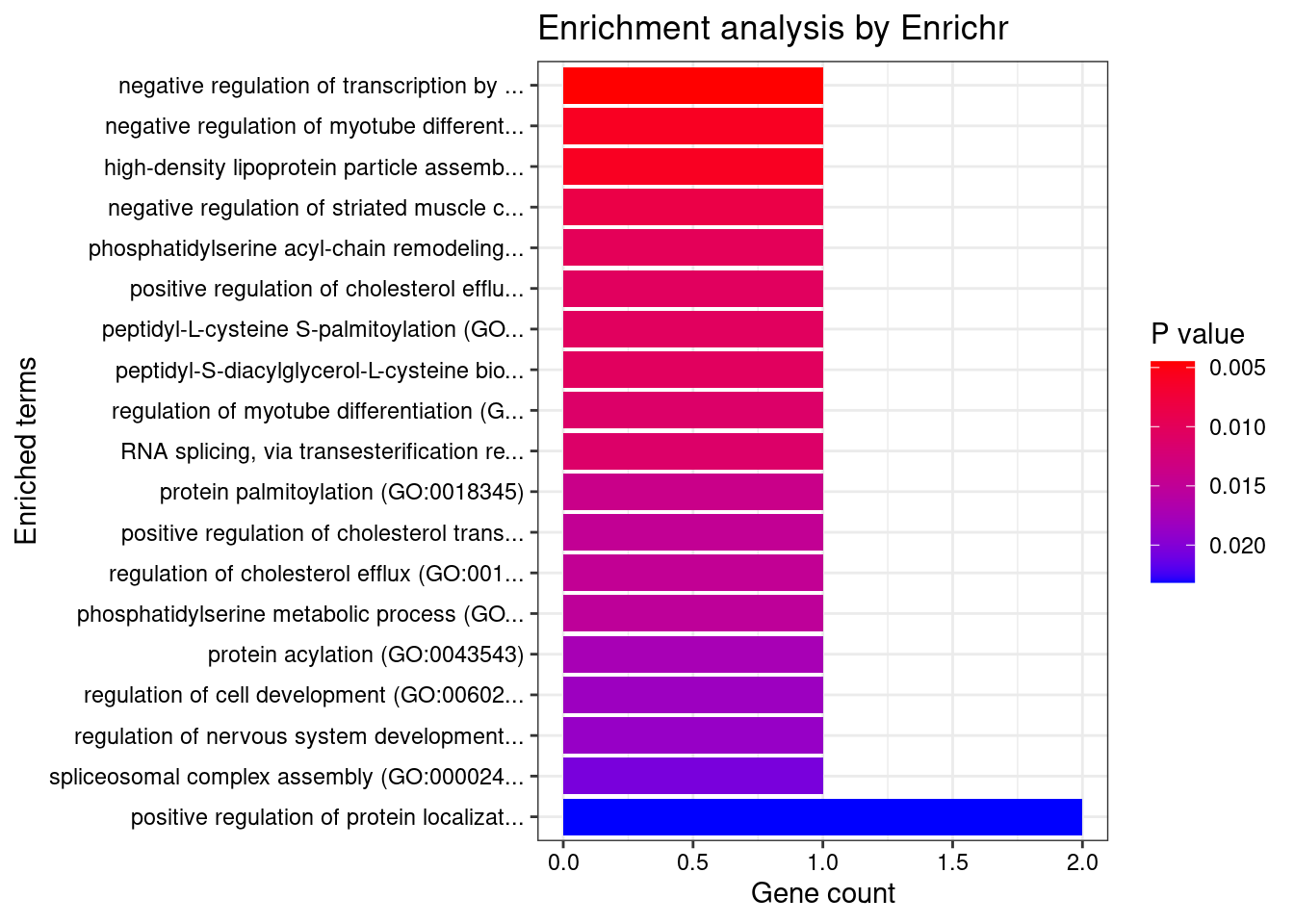
| Version | Author | Date |
|---|---|---|
| 4ded2ef | wesleycrouse | 2022-07-19 |
Endocrine

Number of cTWAS Genes in Tissue Group: 14

Uploading data to Enrichr... Done.
  Querying GO_Biological_Process_2021... Done.
Parsing results... Done.

GO_Biological_Process_2021

                                                   Term Overlap Adjusted.P.value       Genes
1       cellular response to acid chemical (GO:0071229)    2/28       0.01310465 RPTOR;CPEB1
2                   response to amino acid (GO:0043200)    2/32       0.01310465 RPTOR;CPEB1
3 cellular response to amino acid stimulus (GO:0071230)    2/34       0.01310465 RPTOR;CPEB1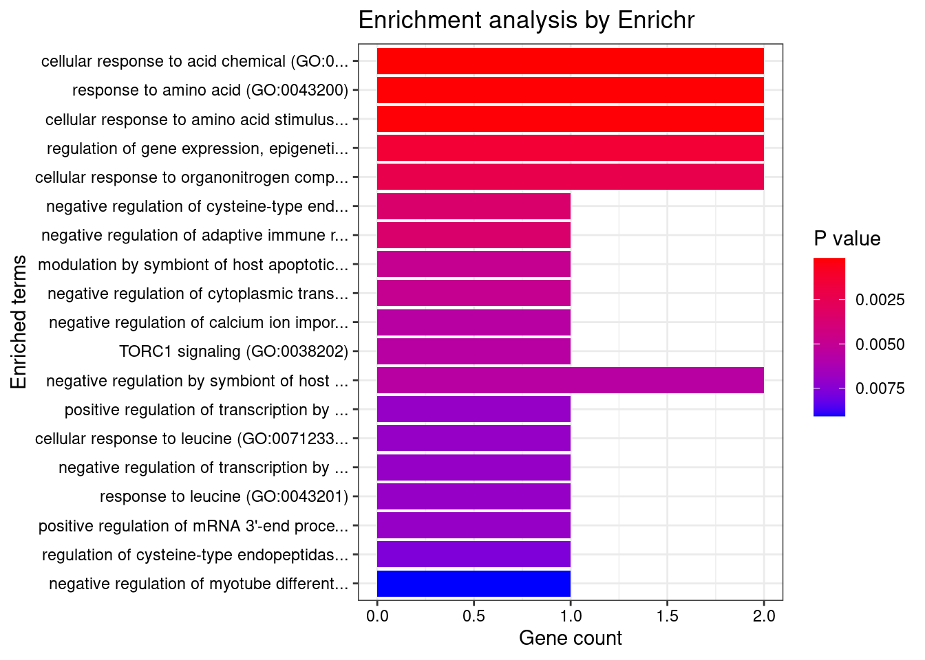
| Version | Author | Date |
|---|---|---|
| 4ded2ef | wesleycrouse | 2022-07-19 |
Cardiovascular

Number of cTWAS Genes in Tissue Group: 26

Uploading data to Enrichr... Done.
  Querying GO_Biological_Process_2021... Done.
Parsing results... Done.

GO_Biological_Process_2021

[1] Term             Overlap          Adjusted.P.value Genes
<0 rows> (or 0-length row.names)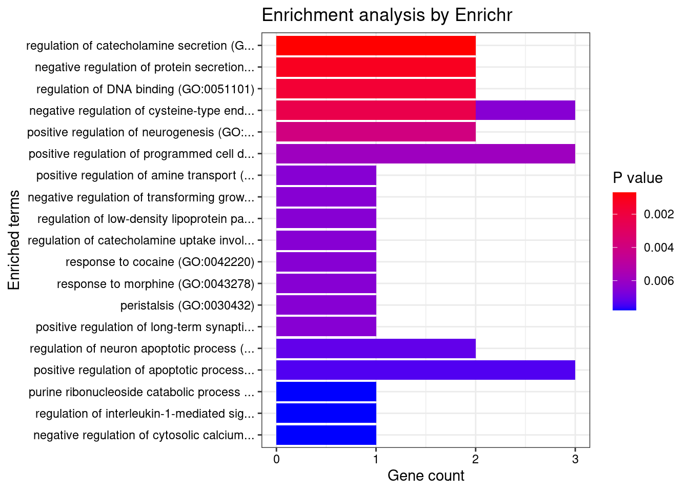
| Version | Author | Date |
|---|---|---|
| 4ded2ef | wesleycrouse | 2022-07-19 |
CNS

Number of cTWAS Genes in Tissue Group: 43

Uploading data to Enrichr... Done.
  Querying GO_Biological_Process_2021... Done.
Parsing results... Done.

GO_Biological_Process_2021

[1] Term             Overlap          Adjusted.P.value Genes
<0 rows> (or 0-length row.names)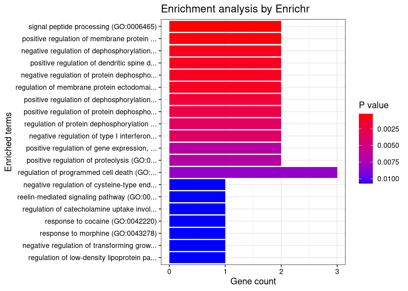
| Version | Author | Date |
|---|---|---|
| 4ded2ef | wesleycrouse | 2022-07-19 |
None

Number of cTWAS Genes in Tissue Group: 33

Uploading data to Enrichr... Done.
  Querying GO_Biological_Process_2021... Done.
Parsing results... Done.

GO_Biological_Process_2021

[1] Term             Overlap          Adjusted.P.value Genes
<0 rows> (or 0-length row.names)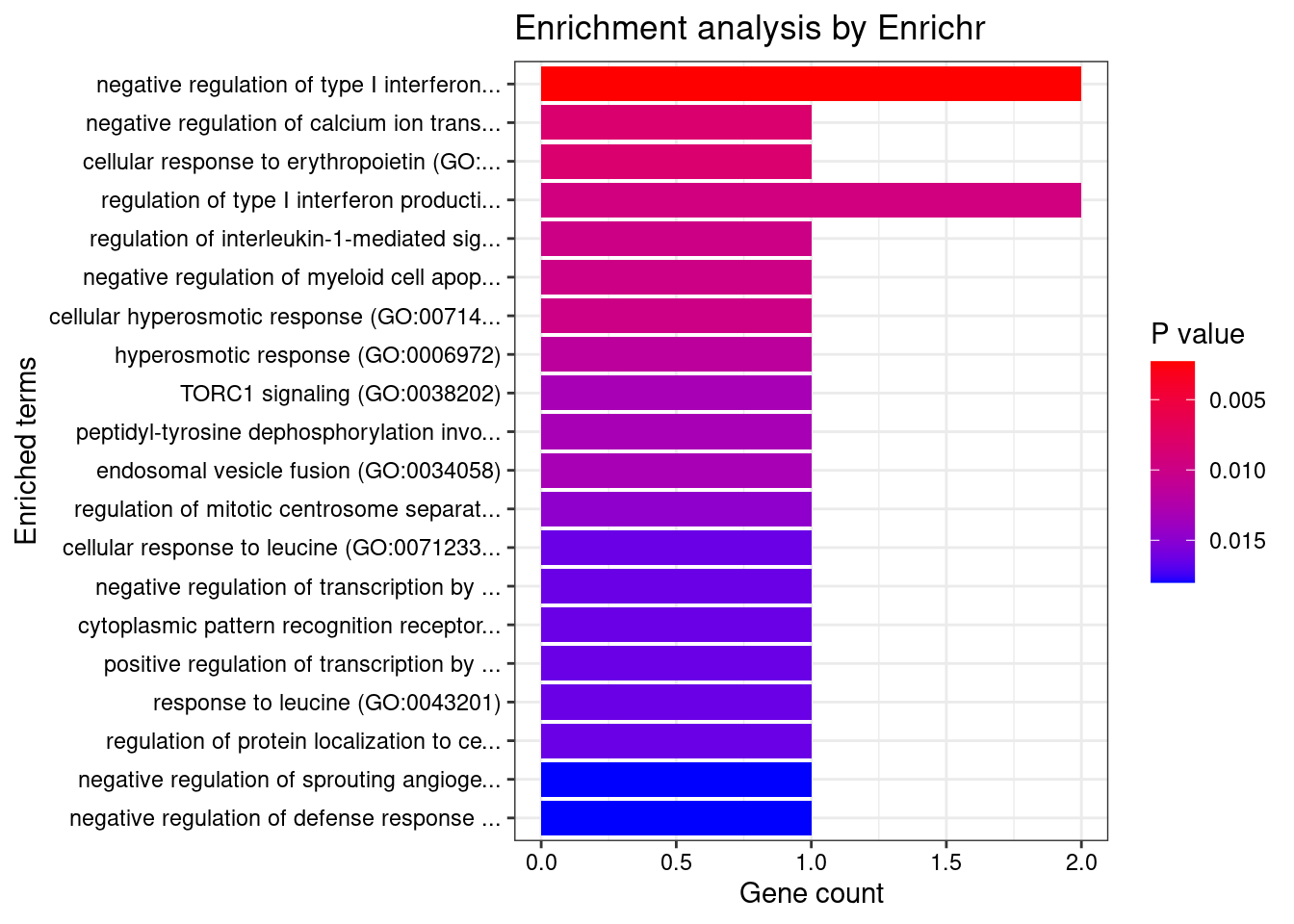
| Version | Author | Date |
|---|---|---|
| 4ded2ef | wesleycrouse | 2022-07-19 |
Skin

Number of cTWAS Genes in Tissue Group: 22

Uploading data to Enrichr... Done.
  Querying GO_Biological_Process_2021... Done.
Parsing results... Done.

GO_Biological_Process_2021

[1] Term             Overlap          Adjusted.P.value Genes
<0 rows> (or 0-length row.names)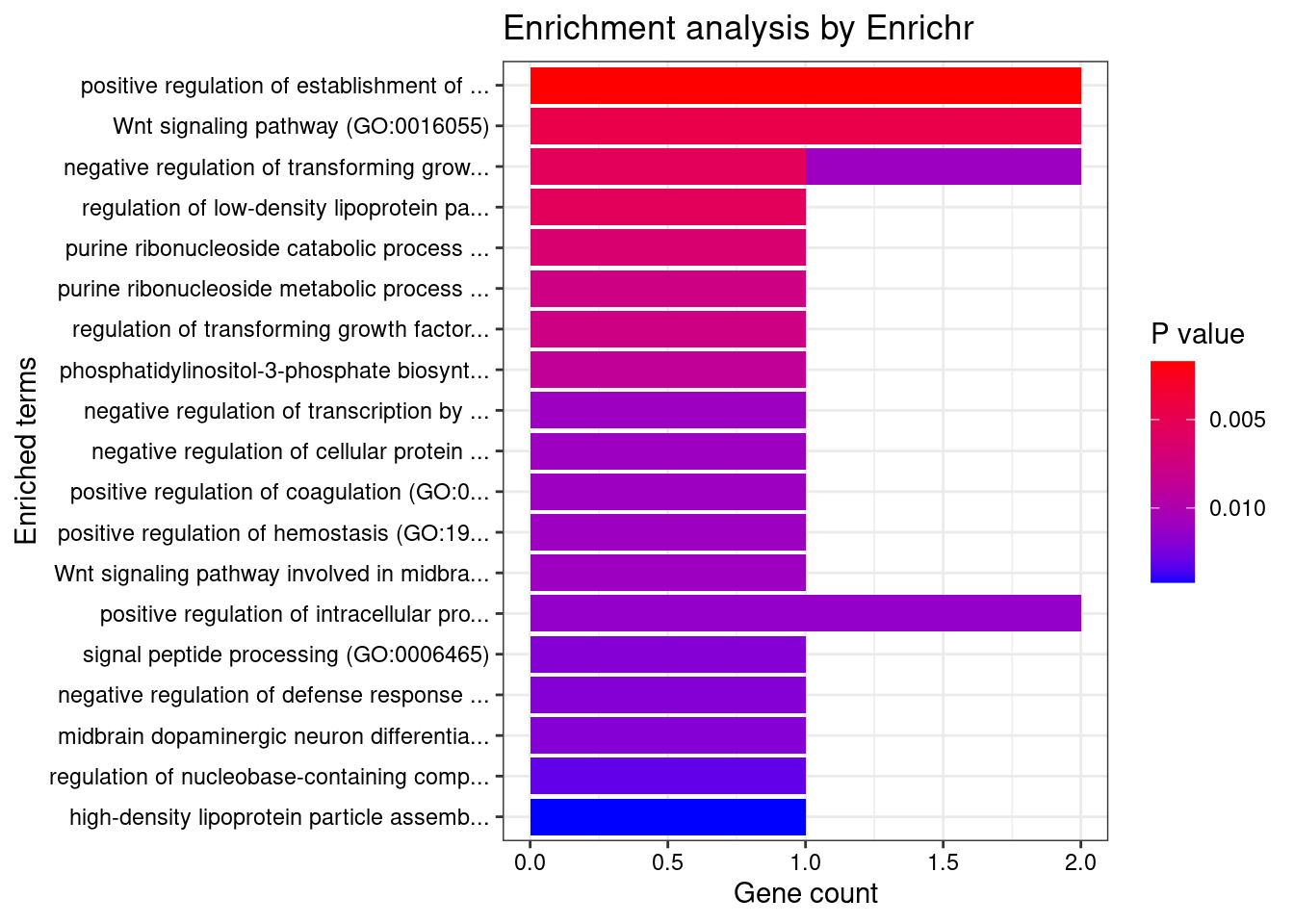
| Version | Author | Date |
|---|---|---|
| 4ded2ef | wesleycrouse | 2022-07-19 |
Blood or Immune

Number of cTWAS Genes in Tissue Group: 10

Uploading data to Enrichr... Done.
  Querying GO_Biological_Process_2021... Done.
Parsing results... Done.

GO_Biological_Process_2021

                                                             Term Overlap Adjusted.P.value        Genes
1 positive regulation of gene expression, epigenetic (GO:0045815)    2/57       0.03043340 POLR2E;SF3B1
2          regulation of gene expression, epigenetic (GO:0040029)    2/82       0.03145299 POLR2E;SF3B1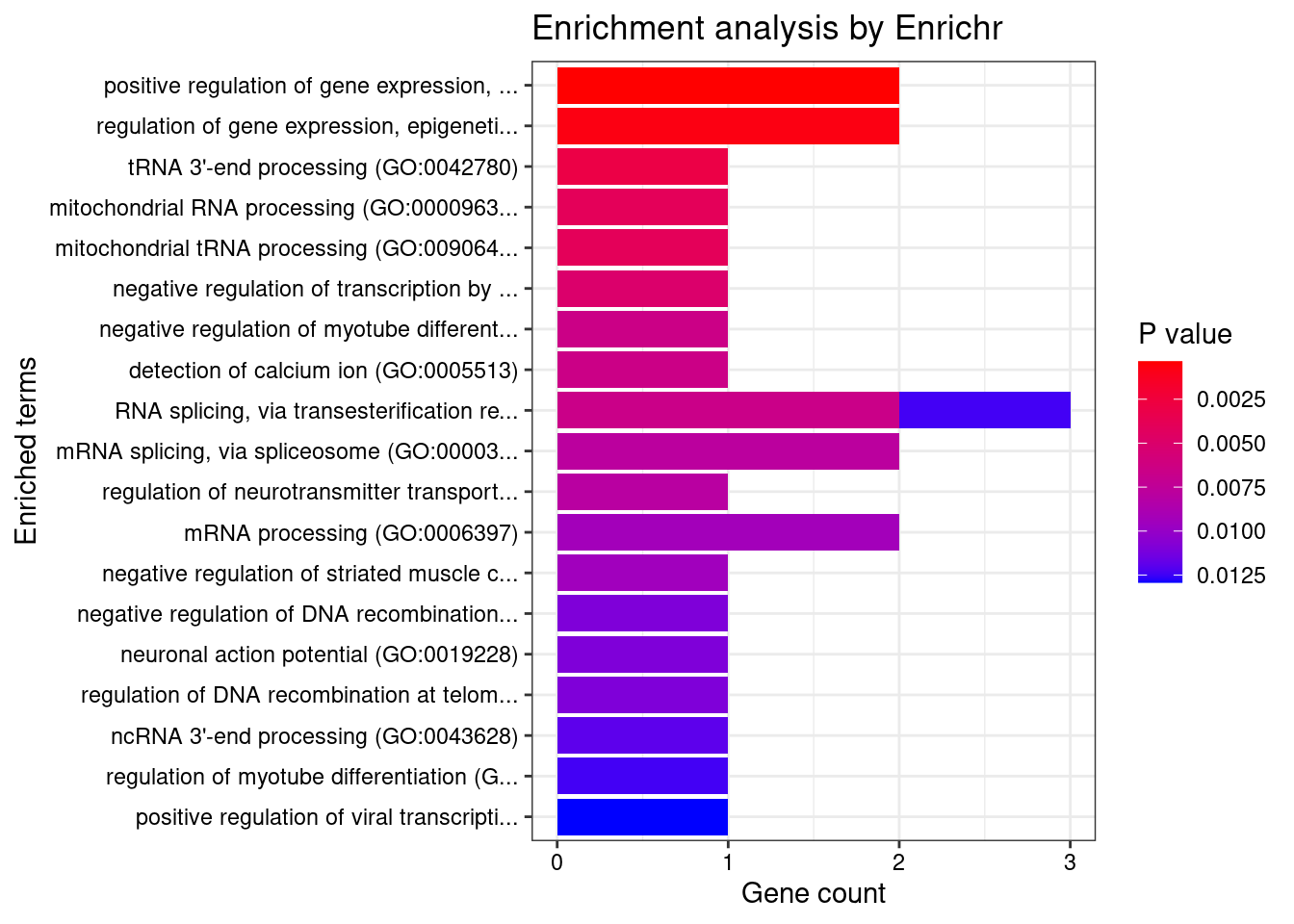
| Version | Author | Date |
|---|---|---|
| 4ded2ef | wesleycrouse | 2022-07-19 |
Digestive

Number of cTWAS Genes in Tissue Group: 24

Uploading data to Enrichr... Done.
  Querying GO_Biological_Process_2021... Done.
Parsing results... Done.

GO_Biological_Process_2021

[1] Term             Overlap          Adjusted.P.value Genes
<0 rows> (or 0-length row.names)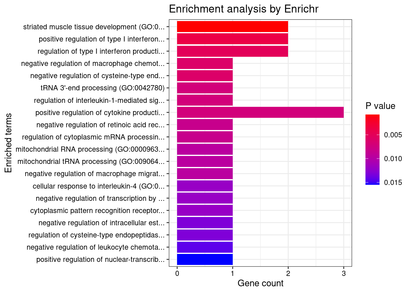
| Version | Author | Date |
|---|---|---|
| 4ded2ef | wesleycrouse | 2022-07-19 |
if (exists("group_enrichment_results")){
  save(group_enrichment_results, file=paste0("group_enrichment_results_", trait_id, ".RData"))
}
KEGG
for (group in names(df_group)){
  cat(paste0(group, "\n\n"))

  ctwas_genes_group <- df_group[[group]]$ctwas
  background_group <- df_group[[group]]$background

  cat(paste0("Number of cTWAS Genes in Tissue Group: ", length(ctwas_genes_group), "\n\n"))

  databases <- c("pathway_KEGG")

  enrichResult <- WebGestaltR(enrichMethod="ORA", organism="hsapiens",
                              interestGene=ctwas_genes_group, referenceGene=background_group,
                              enrichDatabase=databases, interestGeneType="genesymbol",
                              referenceGeneType="genesymbol", isOutput=F)

  if (!is.null(enrichResult)){
    print(enrichResult[,c("description", "size", "overlap", "FDR", "userId")])
  }

  cat("\n")
}
Adipose
Number of cTWAS Genes in Tissue Group: 9
Loading the functional categories...
Loading the ID list...
Loading the reference list...
Performing the enrichment analysis...Warning in oraEnrichment(interestGeneList, referenceGeneList, geneSet, minNum = minNum, : No significant gene set is identified based on FDR 0.05!
Endocrine

Number of cTWAS Genes in Tissue Group: 14

Loading the functional categories...
Loading the ID list...
Loading the reference list...
Performing the enrichment analysis...
Warning in oraEnrichment(interestGeneList, referenceGeneList, geneSet, minNum = minNum, : No significant gene set is identified based on FDR 0.05!
Cardiovascular

Number of cTWAS Genes in Tissue Group: 26

Loading the functional categories...
Loading the ID list...
Loading the reference list...
Performing the enrichment analysis...
Warning in oraEnrichment(interestGeneList, referenceGeneList, geneSet, minNum = minNum, : No significant gene set is identified based on FDR 0.05!
CNS

Number of cTWAS Genes in Tissue Group: 43

Loading the functional categories...
Loading the ID list...
Loading the reference list...
Performing the enrichment analysis...
Warning in oraEnrichment(interestGeneList, referenceGeneList, geneSet, minNum = minNum, : No significant gene set is identified based on FDR 0.05!
None

Number of cTWAS Genes in Tissue Group: 33

Loading the functional categories...
Loading the ID list...
Loading the reference list...
Performing the enrichment analysis...
Warning in oraEnrichment(interestGeneList, referenceGeneList, geneSet, minNum = minNum, : No significant gene set is identified based on FDR 0.05!
Skin

Number of cTWAS Genes in Tissue Group: 22

Loading the functional categories...
Loading the ID list...
Loading the reference list...
Performing the enrichment analysis...
Warning in oraEnrichment(interestGeneList, referenceGeneList, geneSet, minNum = minNum, : No significant gene set is identified based on FDR 0.05!
Blood or Immune

Number of cTWAS Genes in Tissue Group: 10

Loading the functional categories...
Loading the ID list...
Loading the reference list...
Performing the enrichment analysis...
Warning in oraEnrichment(interestGeneList, referenceGeneList, geneSet, minNum = minNum, : No significant gene set is identified based on FDR 0.05!
Digestive

Number of cTWAS Genes in Tissue Group: 24

Loading the functional categories...
Loading the ID list...
Loading the reference list...
Performing the enrichment analysis...
Warning in oraEnrichment(interestGeneList, referenceGeneList, geneSet, minNum = minNum, : No significant gene set is identified based on FDR 0.05!DisGeNET
for (group in names(df_group)){
  cat(paste0(group, "\n\n"))

  ctwas_genes_group <- df_group[[group]]$ctwas

  cat(paste0("Number of cTWAS Genes in Tissue Group: ", length(ctwas_genes_group), "\n\n"))

  res_enrich <- disease_enrichment(entities=ctwas_genes_group, vocabulary = "HGNC", database = "CURATED")

  if (any(res_enrich@qresult$FDR < 0.05)){
    print(res_enrich@qresult[res_enrich@qresult$FDR < 0.05, c("Description", "FDR", "Ratio",  "BgRatio")])
  }

  cat("\n")
}
Gene sets curated by Macarthur Lab
gene_set_dir <- "/project2/mstephens/wcrouse/gene_sets/"
gene_set_files <- c("gwascatalog.tsv",
                    "mgi_essential.tsv",
                    "core_essentials_hart.tsv",
                    "clinvar_path_likelypath.tsv",
                    "fda_approved_drug_targets.tsv")

for (group in names(df_group)){
  cat(paste0(group, "\n\n"))

  ctwas_genes_group <- df_group[[group]]$ctwas
  background_group <- df_group[[group]]$background

  cat(paste0("Number of cTWAS Genes in Tissue Group: ", length(ctwas_genes_group), "\n\n"))

  gene_sets <- lapply(gene_set_files, function(x){as.character(read.table(paste0(gene_set_dir, x))[,1])})
  names(gene_sets) <- sapply(gene_set_files, function(x){unlist(strsplit(x, "[.]"))[1]})

  gene_lists <- list(ctwas_genes_group=ctwas_genes_group)

  #genes in gene_sets filtered to ensure inclusion in background
  gene_sets <- lapply(gene_sets, function(x){x[x %in% background_group]})

  #hypergeometric test
  hyp_score <- data.frame()
  size <- c()
  ngenes <- c()

  for (i in 1:length(gene_sets)) {
    for (j in 1:length(gene_lists)){
      group1 <- length(gene_sets[[i]])
      group2 <- length(as.vector(gene_lists[[j]]))
      size <- c(size, group1)
      Overlap <- length(intersect(gene_sets[[i]],as.vector(gene_lists[[j]])))
      ngenes <- c(ngenes, Overlap)
      Total <- length(background_group)
      hyp_score[i,j] <- phyper(Overlap-1, group2, Total-group2, group1,lower.tail=F)
    }
  }
  rownames(hyp_score) <- names(gene_sets)
  colnames(hyp_score) <- names(gene_lists)

  #multiple testing correction
  hyp_score_padj <- apply(hyp_score,2, p.adjust, method="BH", n=(nrow(hyp_score)*ncol(hyp_score)))
  hyp_score_padj <- as.data.frame(hyp_score_padj)
  hyp_score_padj$gene_set <- rownames(hyp_score_padj)
  hyp_score_padj$nset <- size
  hyp_score_padj$ngenes <- ngenes
  hyp_score_padj$percent <- ngenes/size

  hyp_score_padj <- hyp_score_padj[order(hyp_score_padj$ctwas_genes),]
  colnames(hyp_score_padj)[1] <- "padj"
  hyp_score_padj <- hyp_score_padj[,c(2:5,1)]
  rownames(hyp_score_padj)<- NULL

  print(hyp_score_padj)

  cat("\n")
}
Adipose
Number of cTWAS Genes in Tissue Group: 9
gene_set nset ngenes percent padj
1 core_essentials_hart 195 1 0.0051282051 0.689294
2 gwascatalog 4224 4 0.0009469697 1.000000
3 mgi_essential 1578 1 0.0006337136 1.000000
4 clinvar_path_likelypath 1978 1 0.0005055612 1.000000
5 fda_approved_drug_targets 238 0 0.0000000000 1.000000
Endocrine
Number of cTWAS Genes in Tissue Group: 14
gene_set nset ngenes percent padj
1 gwascatalog 5123 9 0.001756783 0.1279214
2 core_essentials_hart 222 1 0.004504505 0.4851083
3 mgi_essential 1891 2 0.001057641 0.9348287
4 clinvar_path_likelypath 2349 0 0.000000000 1.0000000
5 fda_approved_drug_targets 281 0 0.000000000 1.0000000
Cardiovascular
Number of cTWAS Genes in Tissue Group: 26
gene_set nset ngenes percent padj
1 gwascatalog 4959 20 0.004033071 0.0001246963
2 mgi_essential 1875 5 0.002666667 0.4348362586
3 core_essentials_hart 234 1 0.004273504 0.4348362586
4 clinvar_path_likelypath 2277 5 0.002195872 0.4348362586
5 fda_approved_drug_targets 264 1 0.003787879 0.4348362586
CNS
Number of cTWAS Genes in Tissue Group: 43
gene_set nset ngenes percent padj
1 gwascatalog 5169 22 0.004256142 0.1182018
2 mgi_essential 1963 4 0.002037697 0.8559578
3 core_essentials_hart 231 1 0.004329004 0.8559578
4 clinvar_path_likelypath 2401 5 0.002082466 0.8559578
5 fda_approved_drug_targets 298 1 0.003355705 0.8559578
None
Number of cTWAS Genes in Tissue Group: 33
gene_set nset ngenes percent padj
1 gwascatalog 5439 19 0.003493289 0.04019719
2 mgi_essential 2051 5 0.002437835 0.61185588
3 core_essentials_hart 246 1 0.004065041 0.61185588
4 fda_approved_drug_targets 308 1 0.003246753 0.61185588
5 clinvar_path_likelypath 2517 3 0.001191895 0.92621835
Skin
Number of cTWAS Genes in Tissue Group: 22
gene_set nset ngenes percent padj
1 gwascatalog 4830 13 0.0026915114 0.1093410
2 mgi_essential 1809 5 0.0027639580 0.4079455
3 core_essentials_hart 217 1 0.0046082949 0.5005301
4 clinvar_path_likelypath 2205 2 0.0009070295 1.0000000
5 fda_approved_drug_targets 257 0 0.0000000000 1.0000000
Blood or Immune
Number of cTWAS Genes in Tissue Group: 10
gene_set nset ngenes percent padj
1 gwascatalog 4432 6 0.0013537906 0.3902966
2 core_essentials_hart 209 1 0.0047846890 0.3902966
3 mgi_essential 1627 1 0.0006146281 1.0000000
4 clinvar_path_likelypath 2031 1 0.0004923683 1.0000000
5 fda_approved_drug_targets 228 0 0.0000000000 1.0000000
Digestive
Number of cTWAS Genes in Tissue Group: 24
gene_set nset ngenes percent padj
1 gwascatalog 5137 13 0.002530660 0.2346535
2 core_essentials_hart 230 1 0.004347826 0.4811472
3 clinvar_path_likelypath 2374 5 0.002106150 0.4811472
4 fda_approved_drug_targets 290 1 0.003448276 0.4811472
5 mgi_essential 1924 2 0.001039501 0.8475248Analysis of TWAS False Positives by Region
library(ggplot2)

pip_threshold <- 0.5

df_plot <- data.frame(Outcome=c("SNPs", "Genes", "Both", "Neither"), Frequency=rep(0,4))

for (i in 1:length(df)){
  gene_pips <- df[[i]]$gene_pips[df[[i]]$gene_pips$genename %in% df[[i]]$twas,,drop=F]
  gene_pips <- gene_pips[gene_pips$susie_pip < pip_threshold,,drop=F]

  region_pips <- df[[i]]$region_pips
  rownames(region_pips) <- region_pips$region

  gene_pips <- cbind(gene_pips, t(sapply(gene_pips$region_tag, function(x){unlist(region_pips[x,c("gene_pip", "snp_pip")])})))
  gene_pips$gene_pip <- gene_pips$gene_pip - gene_pips$susie_pip #subtract gene pip from region total to get combined pip for other genes in region

  df_plot$Frequency[df_plot$Outcome=="Neither"] <- df_plot$Frequency[df_plot$Outcome=="Neither"] + sum(gene_pips$gene_pip < 0.5 & gene_pips$snp_pip < 0.5)
  df_plot$Frequency[df_plot$Outcome=="Both"] <- df_plot$Frequency[df_plot$Outcome=="Both"] + sum(gene_pips$gene_pip > 0.5 & gene_pips$snp_pip > 0.5)
  df_plot$Frequency[df_plot$Outcome=="SNPs"] <- df_plot$Frequency[df_plot$Outcome=="SNPs"] + sum(gene_pips$gene_pip < 0.5 & gene_pips$snp_pip > 0.5)
  df_plot$Frequency[df_plot$Outcome=="Genes"] <- df_plot$Frequency[df_plot$Outcome=="Genes"] + sum(gene_pips$gene_pip > 0.5 & gene_pips$snp_pip < 0.5)
}

pie <- ggplot(df_plot, aes(x="", y=Frequency, fill=Outcome)) + geom_bar(width = 1, stat = "identity")
pie <- pie + coord_polar("y", start=0) + theme_minimal() + theme(axis.title.y=element_blank())
pie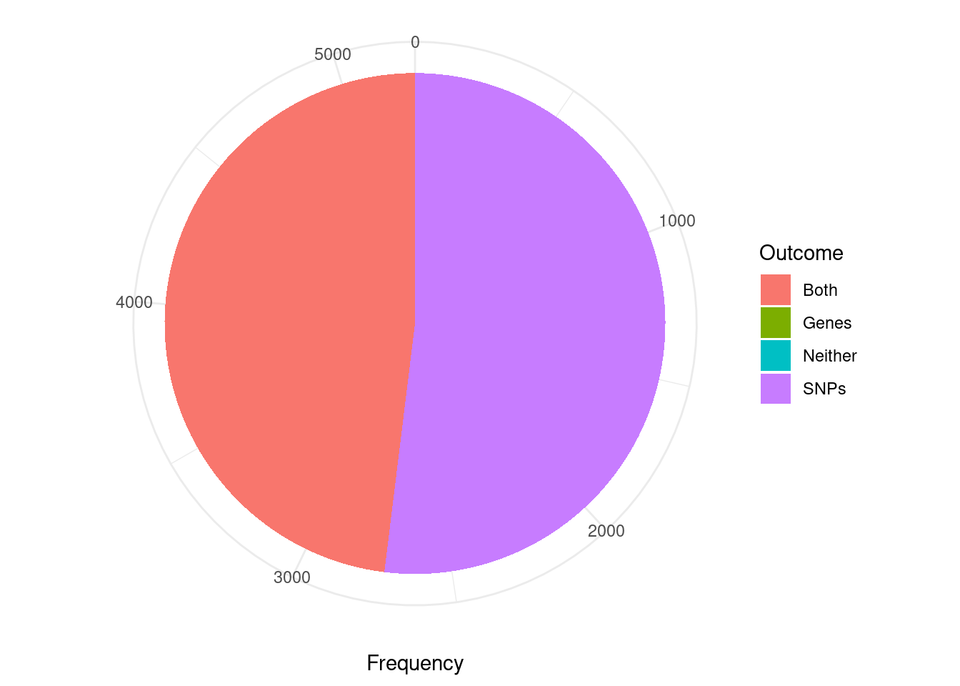
| Version | Author | Date |
|---|---|---|
| 4ded2ef | wesleycrouse | 2022-07-19 |
Analysis of TWAS False Positives by Credible Set
cTWAS is using susie settings that mask credible sets consisting of variables with minimum pairwise correlations below a specified threshold. The default threshold is 0.5. I think this is intended to mask credible sets with “diffuse” support. As a consequence, many of the genes considered here (TWAS false positives; significant z score but low PIP) are not assigned to a credible set (have cs_index=0). For this reason, the first figure is not really appropriate for answering the question “are TWAS false positives due to SNPs or genes”.
The second figure includes only TWAS genes that are assigned to a reported causal set (i.e. they are in a “pure” causal set with high pairwise correlations). I think that this figure is closer to the intended analysis. However, it may be biased in some way because we have excluded many TWAS false positive genes that are in “impure” credible sets.
Some alternatives to these figures include the region-based analysis in the previous section; or re-analysis with lower/no minimum pairwise correlation threshold (“min_abs_corr” option in susie_get_cs) for reporting credible sets.
library(ggplot2)

####################
#using only genes assigned to a credible set

pip_threshold <- 0.5

df_plot <- data.frame(Outcome=c("SNPs", "Genes", "Both", "Neither"), Frequency=rep(0,4))

for (i in 1:length(df)){
  gene_pips <- df[[i]]$gene_pips[df[[i]]$gene_pips$genename %in% df[[i]]$twas,,drop=F]
  gene_pips <- gene_pips[gene_pips$susie_pip < pip_threshold,,drop=F]

  #exclude genes that are not assigned to a credible set, cs_index==0
  gene_pips <- gene_pips[as.numeric(sapply(gene_pips$region_cs_tag, function(x){rev(unlist(strsplit(x, "_")))[1]}))!=0,]

  region_cs_pips <- df[[i]]$region_cs_pips
  rownames(region_cs_pips) <- region_cs_pips$region_cs

  gene_pips <- cbind(gene_pips, t(sapply(gene_pips$region_cs_tag, function(x){unlist(region_cs_pips[x,c("gene_pip", "snp_pip")])})))
  gene_pips$gene_pip <- gene_pips$gene_pip - gene_pips$susie_pip #subtract gene pip from causal set total to get combined pip for other genes in causal set

  plot_cutoff <- 0.5

  df_plot$Frequency[df_plot$Outcome=="Neither"] <- df_plot$Frequency[df_plot$Outcome=="Neither"] + sum(gene_pips$gene_pip < plot_cutoff & gene_pips$snp_pip < plot_cutoff)
  df_plot$Frequency[df_plot$Outcome=="Both"] <- df_plot$Frequency[df_plot$Outcome=="Both"] + sum(gene_pips$gene_pip > plot_cutoff & gene_pips$snp_pip > plot_cutoff)
  df_plot$Frequency[df_plot$Outcome=="SNPs"] <- df_plot$Frequency[df_plot$Outcome=="SNPs"] + sum(gene_pips$gene_pip < plot_cutoff & gene_pips$snp_pip > plot_cutoff)
  df_plot$Frequency[df_plot$Outcome=="Genes"] <- df_plot$Frequency[df_plot$Outcome=="Genes"] + sum(gene_pips$gene_pip > plot_cutoff & gene_pips$snp_pip < plot_cutoff)
}

pie <- ggplot(df_plot, aes(x="", y=Frequency, fill=Outcome)) + geom_bar(width = 1, stat = "identity")
pie <- pie + coord_polar("y", start=0) + theme_minimal() + theme(axis.title.y=element_blank())
pie
| Version | Author | Date |
|---|---|---|
| 4ded2ef | wesleycrouse | 2022-07-19 |
cTWAS genes without genome-wide significant SNP nearby
novel_genes <- data.frame(genename=as.character(), weight=as.character(), susie_pip=as.numeric(), snp_maxz=as.numeric())

for (i in 1:length(df)){
  gene_pips <- df[[i]]$gene_pips[df[[i]]$gene_pips$genename %in% df[[i]]$ctwas,,drop=F]

  region_pips <- df[[i]]$region_pips
  rownames(region_pips) <- region_pips$region

  gene_pips <- cbind(gene_pips, sapply(gene_pips$region_tag, function(x){region_pips[x,"snp_maxz"]}))
  names(gene_pips)[ncol(gene_pips)] <- "snp_maxz"

  if (nrow(gene_pips)>0){
    gene_pips$weight <- names(df)[i]
    gene_pips <- gene_pips[gene_pips$snp_maxz < qnorm(1-(5E-8/2), lower=T),c("genename", "weight", "susie_pip", "snp_maxz")]

    novel_genes <- rbind(novel_genes, gene_pips)
  }
}

novel_genes_summary <- data.frame(genename=unique(novel_genes$genename))
novel_genes_summary$nweights <- sapply(novel_genes_summary$genename, function(x){length(novel_genes$weight[novel_genes$genename==x])})
novel_genes_summary$weights <- sapply(novel_genes_summary$genename, function(x){paste(novel_genes$weight[novel_genes$genename==x],collapse=", ")})

novel_genes_summary <- novel_genes_summary[order(-novel_genes_summary$nweights),]
novel_genes_summary[,c("genename","nweights")]
genename nweights
2 BHLHE41 18
17 TMEM222 15
8 ELAC2 9
7 FANCI 8
19 SYTL1 6
33 PCBP2 6
10 CAAP1 5
14 SPECC1 5
27 FEZF1 4
31 PTPA 4
37 VPS8 4
51 LPCAT4 4
12 PDXDC1 3
23 WBP2 3
11 SOX5 2
15 ENPP4 2
26 GALNT2 2
30 NPIPA1 2
40 CNNM1 2
46 MFAP3L 2
53 EPO 2
57 FAM205A 2
1 OSBPL10 1
3 FAM83H 1
4 ZDHHC8 1
5 NGF 1
6 PRKD3 1
9 CWC25 1
13 ZZEF1 1
16 KCNB1 1
18 JSRP1 1
20 TMEM81 1
21 PACSIN3 1
22 TBC1D29 1
24 ZCCHC2 1
25 KCNG1 1
28 LRP8 1
29 SSPN 1
32 CCDC6 1
34 RCBTB1 1
35 FOXO6 1
36 C19orf35 1
38 GAL 1
39 GIGYF1 1
41 LAMTOR2 1
42 ARL6 1
43 KLHL9 1
44 POLR2E 1
45 SGCD 1
47 CALD1 1
48 SVIL 1
49 C5 1
50 C10orf11 1
52 DOT1L 1
54 UBXN2B 1
55 MAMDC2 1
56 PTPRT 1
58 RBBP5 1
59 EPN2 1
60 GNAI2 1
61 LSMEM2 1
62 PIK3C2B 1
63 C5orf30 1
64 WNT9B 1
65 FAM117B 1
66 GSX2 1
67 KCNMB4 1
68 IFRD2 1
69 FAM83H-AS1 1
70 CLIC5 1Tissue-specificity for cTWAS genes
gene_pips_by_weight <- data.frame(genename=as.character(ctwas_genes))

for (i in 1:length(df)){
  gene_pips <- df[[i]]$gene_pips
  gene_pips <- gene_pips[match(ctwas_genes, gene_pips$genename),,drop=F]

  gene_pips_by_weight <- cbind(gene_pips_by_weight, gene_pips$susie_pip)
  names(gene_pips_by_weight)[ncol(gene_pips_by_weight)] <- names(df)[i]
}

gene_pips_by_weight <- as.matrix(gene_pips_by_weight[,-1])
rownames(gene_pips_by_weight) <- ctwas_genes

#handing missing values
gene_pips_by_weight_bkup <- gene_pips_by_weight
gene_pips_by_weight[is.na(gene_pips_by_weight)] <- 0

#number of tissues with PIP>0.5 for cTWAS genes
ctwas_frequency <- rowSums(gene_pips_by_weight>0.5)

pdf(file = "output/SCZ_tissue_specificity.pdf", width = 3.5, height = 2.5)

par(mar=c(4.6, 3.6, 1.1, 0.6))

hist(ctwas_frequency, col="grey", breaks=0:max(ctwas_frequency),
     #xlim=c(0,ncol(gene_pips_by_weight)),
     xlab="Number of Tissues\nwith PIP>0.5",
     ylab="Number of cTWAS Genes",
     main="SCZ")

dev.off()
png
2 #heatmap of gene PIPs
cluster_ctwas_genes <- hclust(dist(gene_pips_by_weight))
cluster_ctwas_weights <- hclust(dist(t(gene_pips_by_weight)))
plot(cluster_ctwas_weights, cex=0.6)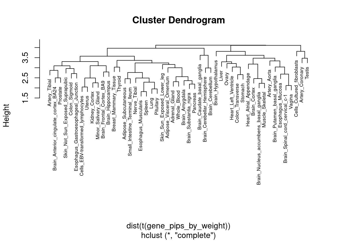
plot(cluster_ctwas_genes, cex=0.6, labels=F)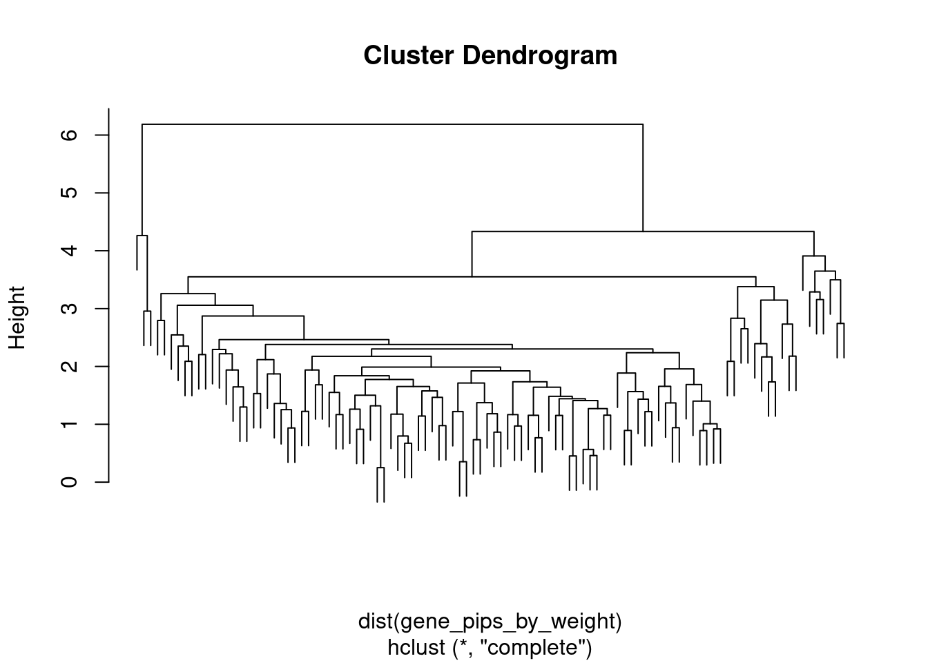
par(mar=c(14.1, 4.1, 4.1, 2.1))

image(t(gene_pips_by_weight[rev(cluster_ctwas_genes$order),rev(cluster_ctwas_weights$order)]),
      axes=F)
mtext(text=colnames(gene_pips_by_weight)[cluster_ctwas_weights$order], side=1, line=0.3, at=seq(0,1,1/(ncol(gene_pips_by_weight)-1)), las=2, cex=0.8)
mtext(text=rownames(gene_pips_by_weight)[cluster_ctwas_genes$order], side=2, line=0.3, at=seq(0,1,1/(nrow(gene_pips_by_weight)-1)), las=1, cex=0.4)
| Version | Author | Date |
|---|---|---|
| 4ded2ef | wesleycrouse | 2022-07-19 |
cTWAS genes with highest proportion of total PIP on a single tissue
#genes with highest proportion of PIP on a single tissue
gene_pips_proportion <- gene_pips_by_weight/rowSums(gene_pips_by_weight)

proportion_table <- data.frame(genename=as.character(rownames(gene_pips_proportion)))
proportion_table$max_pip_prop <- apply(gene_pips_proportion,1,max)
proportion_table$max_weight <- colnames(gene_pips_proportion)[apply(gene_pips_proportion,1,which.max)]

proportion_table[order(-proportion_table$max_pip_prop),]
genename max_pip_prop max_weight
6 PPP1R18 0.85754212 Adipose_Visceral_Omentum
11 NGF 0.82764122 Artery_Aorta
87 GNAI2 0.80204311 Ovary
103 NRGN 0.79322366 Thyroid
48 SPCS1 0.76563850 Brain_Cortex
99 IFRD2 0.68726838 Stomach
59 ZNF844 0.63433283 Brain_Spinal_cord_cervical_c-1
45 SSPN 0.59761140 Brain_Cerebellum
78 PAK6 0.58049280 Heart_Left_Ventricle
72 SVIL 0.54040823 Esophagus_Gastroesophageal_Junction
95 WNT9B 0.51776488 Skin_Not_Sun_Exposed_Suprapubic
68 SGCD 0.50726594 Colon_Sigmoid
9 ZDHHC8 0.49441601 Adipose_Visceral_Omentum
30 KCNB1 0.48187006 Artery_Tibial
79 EPO 0.44672493 Prostate
90 ZNF878 0.44333009 Prostate
102 CLIC5 0.44182641 Thyroid
77 DOT1L 0.42728249 Heart_Atrial_Appendage
82 PPM1A 0.42303385 Liver
40 KCNG1 0.42140369 Brain_Caudate_basal_ganglia
56 GAL 0.40575634 Brain_Hypothalamus
10 TRIM27 0.39920640 Adrenal_Gland
1 OSBPL10 0.39550992 Adipose_Subcutaneous
33 JSRP1 0.39036231 Brain_Anterior_cingulate_cortex_BA24
41 GALNT2 0.38185801 Brain_Cerebellar_Hemisphere
47 TNFRSF13C 0.37226537 Brain_Cerebellum
14 BNIP3L 0.34495160 Artery_Aorta
73 C5 0.30586853 Esophagus_Mucosa
46 NPIPA1 0.30433468 Stomach
64 ARL6 0.30351812 Cells_Cultured_fibroblasts
96 FAM117B 0.29992001 Skin_Sun_Exposed_Lower_leg
85 RBBP5 0.29908969 Nerve_Tibial
54 C19orf35 0.29435669 Brain_Hippocampus
93 C5orf30 0.29263279 Skin_Not_Sun_Exposed_Suprapubic
84 FAM205A 0.29016194 Skin_Sun_Exposed_Lower_leg
71 CALD1 0.28997491 Esophagus_Gastroesophageal_Junction
62 CACNA1I 0.28882416 Breast_Mammary_Tissue
89 MMP16 0.28427180 Ovary
83 PTPRT 0.28333410 Liver
43 LRP8 0.28292076 Brain_Cerebellum
15 DRD2 0.28273401 Artery_Aorta
88 LSMEM2 0.27364244 Ovary
35 TMEM81 0.25686395 Brain_Caudate_basal_ganglia
12 PRKD3 0.25119058 Artery_Aorta
53 FOXO6 0.24265898 Brain_Frontal_Cortex_BA9
42 FEZF1 0.24188115 Brain_Cerebellum
26 ZZEF1 0.24053945 Artery_Coronary
4 SCAF1 0.22577123 Adipose_Subcutaneous
28 ENPP4 0.22322153 Cells_Cultured_fibroblasts
100 FAM83H-AS1 0.20647676 Testis
91 PIK3C2B 0.19926987 Skin_Not_Sun_Exposed_Suprapubic
94 APOM 0.19606904 Skin_Not_Sun_Exposed_Suprapubic
60 GIGYF1 0.19308115 Breast_Mammary_Tissue
39 ZCCHC2 0.18922142 Brain_Caudate_basal_ganglia
61 CNNM1 0.18901593 Breast_Mammary_Tissue
67 POLR2E 0.18793892 Cells_EBV-transformed_lymphocytes
75 STAT6 0.18629851 Esophagus_Mucosa
65 KLHL9 0.17772308 Cells_Cultured_fibroblasts
7 FAM83H 0.17534085 Adipose_Visceral_Omentum
58 TMEM56 0.17275486 Liver
25 PDXDC1 0.17140872 Heart_Left_Ventricle
51 PCBP2 0.16670101 Brain_Hypothalamus
21 CAAP1 0.16265645 Brain_Hypothalamus
97 GSX2 0.16067736 Skin_Sun_Exposed_Lower_leg
104 CPEB1 0.15000443 Thyroid
70 CNOT1 0.14737910 Colon_Transverse
57 PPP1R16B 0.14261125 Brain_Hypothalamus
69 MFAP3L 0.14013301 Stomach
18 CWC25 0.13984955 Artery_Aorta
36 PACSIN3 0.13280981 Brain_Caudate_basal_ganglia
74 C10orf11 0.13097841 Esophagus_Mucosa
50 CCDC6 0.13038632 Brain_Cortex
101 RPTOR 0.12870234 Testis
63 LAMTOR2 0.12781153 Cells_Cultured_fibroblasts
92 UBE2D3 0.12738642 Skin_Not_Sun_Exposed_Suprapubic
98 KCNMB4 0.12706041 Spleen
52 RCBTB1 0.12459584 Brain_Cortex
23 B3GAT1 0.11904223 Brain_Amygdala
27 SPECC1 0.11644052 Brain_Nucleus_accumbens_basal_ganglia
24 SOX5 0.11372251 Heart_Atrial_Appendage
86 EPN2 0.11335136 Nerve_Tibial
37 TBC1D29 0.10855621 Brain_Caudate_basal_ganglia
38 WBP2 0.10804281 Brain_Caudate_basal_ganglia
76 LPCAT4 0.10573481 Small_Intestine_Terminal_Ileum
20 NGEF 0.10396673 Artery_Coronary
66 CPNE2 0.10291896 Cells_Cultured_fibroblasts
22 PCNX3 0.09399559 Whole_Blood
44 MAP3K11 0.09246357 Brain_Hippocampus
49 PTPA 0.08941664 Brain_Putamen_basal_ganglia
31 PPP1R13B 0.08626519 Brain_Hypothalamus
16 FANCI 0.07839447 Brain_Hypothalamus
19 IRF3 0.07495928 Artery_Aorta
80 UBXN2B 0.07436772 Liver
81 MAMDC2 0.07226292 Liver
29 FURIN 0.07109969 Cells_Cultured_fibroblasts
55 VPS8 0.06012187 Ovary
17 ELAC2 0.05933987 Whole_Blood
34 SYTL1 0.05636650 Breast_Mammary_Tissue
3 BHLHE41 0.05590768 Esophagus_Gastroesophageal_Junction
13 VRK2 0.04996718 Stomach
32 TMEM222 0.04748115 Stomach
2 HIST1H2BN 0.03892226 Adrenal_Gland
5 SF3B1 0.02799773 Brain_Hypothalamus
8 ZNF823 0.02464683 Brain_HypothalamusGenes nearby and nearest to GWAS peaks
#####load positions for all genes on autosomes in ENSEMBL, subset to only protein coding and lncRNA with non-missing HGNC symbol
# library(biomaRt)
#
# ensembl <- useEnsembl(biomart="ENSEMBL_MART_ENSEMBL", dataset="hsapiens_gene_ensembl")
# G_list <- getBM(filters= "chromosome_name", attributes= c("hgnc_symbol","chromosome_name","start_position","end_position","gene_biotype", "ensembl_gene_id", "strand"), values=1:22, mart=ensembl)
#
# save(G_list, file=paste0("G_list_", trait_id, ".RData"))
load(paste0("G_list_", trait_id, ".RData"))

G_list <- G_list[G_list$gene_biotype %in% c("protein_coding"),]
G_list$hgnc_symbol[G_list$hgnc_symbol==""] <- "-"
G_list$tss <- G_list[,c("end_position", "start_position")][cbind(1:nrow(G_list),G_list$strand/2+1.5)]

#####load z scores from the analysis and add positions from the LD reference
# results_dir <- results_dirs[1]
# weight <- rev(unlist(strsplit(results_dir, "/")))[1]
# weight <- unlist(strsplit(weight, split="_nolnc"))
# analysis_id <- paste(trait_id, weight, sep="_")
#
# load(paste0(results_dir, "/", analysis_id, "_expr_z_snp.Rd"))
#
# LDR_dir <- "/project2/mstephens/wcrouse/UKB_LDR_0.1/"
# LDR_files <- list.files(LDR_dir)
# LDR_files <- LDR_files[grep(".Rvar" ,LDR_files)]
#
# z_snp$chrom <- as.integer(NA)
# z_snp$pos <- as.integer(NA)
#
# for (i in 1:length(LDR_files)){
#   print(i)
#
#   LDR_info <- read.table(paste0(LDR_dir, LDR_files[i]), header=T)
#   z_snp_index <- which(z_snp$id %in% LDR_info$id)
#   z_snp[z_snp_index,c("chrom", "pos")] <- t(sapply(z_snp_index, function(x){unlist(LDR_info[match(z_snp$id[x], LDR_info$id),c("chrom", "pos")])}))
# }
#
# z_snp <- z_snp[,c("id", "z", "chrom","pos")]
# save(z_snp, file=paste0("z_snp_pos_", trait_id, ".RData"))
load(paste0("z_snp_pos_", trait_id, ".RData"))

####################
#identify genes within 500kb of genome-wide significant variant ("nearby")
G_list$nearby <- NA

window_size <- 500000

for (chr in 1:22){
  #index genes on chromosome
  G_list_index <- which(G_list$chromosome_name==chr)

  #subset z_snp to chromosome, then subset to significant genome-wide significant variants
  z_snp_chr <- z_snp[z_snp$chrom==chr,,drop=F]
  z_snp_chr <- z_snp_chr[abs(z_snp_chr$z)>qnorm(1-(5E-8/2), lower=T),,drop=F]

  #iterate over genes on chromsome and check if a genome-wide significant SNP is within the window
  for (i in G_list_index){
    window_start <- G_list$start_position[i] - window_size
    window_end <- G_list$end_position[i] + window_size
    G_list$nearby[i] <- any(z_snp_chr$pos>=window_start & z_snp_chr$pos<=window_end)
  }
}

####################
#identify genes that are nearest to lead genome-wide significant variant ("nearest")
G_list$nearest <- F
G_list$distance <- Inf
G_list$which_nearest <- NA

window_size <- 500000

n_peaks <- 0

for (chr in 1:22){
  #index genes on chromosome
  G_list_index <- which(G_list$chromosome_name==chr & G_list$gene_biotype=="protein_coding")

  #subset z_snp to chromosome, then subset to significant genome-wide significant variants
  z_snp_chr <- z_snp[z_snp$chrom==chr,,drop=F]
  z_snp_chr <- z_snp_chr[abs(z_snp_chr$z)>qnorm(1-(5E-8/2), lower=T),,drop=F]

  while (nrow(z_snp_chr)>0){
    n_peaks <- n_peaks + 1

    lead_index <- which.max(abs(z_snp_chr$z))
    lead_position <- z_snp_chr$pos[lead_index]

    distances <- sapply(G_list_index, function(i){
      if (lead_position >= G_list$start_position[i] & lead_position <= G_list$end_position[i]){
        distance <- 0
      } else {
        distance <- min(abs(G_list$start_position[i] - lead_position), abs(G_list$end_position[i] - lead_position))
      }
      distance
    })

    min_distance <- min(distances)

    G_list$nearest[G_list_index[distances==min_distance]] <- T

    nearest_genes <- paste0(G_list$hgnc_symbol[G_list_index[distances==min_distance]], collapse=", ")

    update_index <- which(G_list$distance[G_list_index] > distances)
    G_list$distance[G_list_index][update_index] <- distances[update_index]
    G_list$which_nearest[G_list_index][update_index] <- nearest_genes

    window_start <- lead_position - window_size
    window_end <- lead_position + window_size
    z_snp_chr <- z_snp_chr[!(z_snp_chr$pos>=window_start & z_snp_chr$pos<=window_end),,drop=F]
  }
}

G_list$distance[G_list$distance==Inf] <- NA

#report number of GWAS peaks
sum(n_peaks)
[1] 161Enrichment analysis using known silver standard genes
save.image("workspace20.RData")

# known_genes <- as.data.frame(readxl::read_xlsx("data/Supplementary Table 20 - Prioritised Genes.xlsx", sheet="ST20 all criteria"))
# known_genes <- as.character(unique(known_genes$Symbol.ID[known_genes$Prioritised==1]))

known_genes <- as.data.frame(readxl::read_xlsx("data/Supplementary_Table_12_prioritized_genes.xlsx", sheet="ST12 all criteria"))
known_genes <- as.character(unique(known_genes$Symbol.ID[known_genes$Prioritised==1]))

dbs <- c("GO_Biological_Process_2021")
GO_enrichment <- enrichr(known_genes, dbs)
Uploading data to Enrichr... Done.
Querying GO_Biological_Process_2021... Done.
Parsing results... Done.for (db in dbs){
cat(paste0(db, "\n\n"))
enrich_results <- GO_enrichment[[db]]
enrich_results <- enrich_results[enrich_results$Adjusted.P.value<0.05,c("Term", "Overlap", "Adjusted.P.value", "Genes")]
print(enrich_results)
print(plotEnrich(GO_enrichment[[db]]))
}GO_Biological_Process_2021
Term Overlap Adjusted.P.value Genes
1 presynaptic membrane assembly (GO:0097105) 3/10 0.01429521 PTPRD;NLGN4X;IL1RAPL1
2 presynaptic membrane organization (GO:0097090) 3/11 0.01429521 PTPRD;NLGN4X;IL1RAPL1
3 regulation of presynapse assembly (GO:1905606) 3/18 0.02742401 PTPRD;IL1RAPL1;LRRC4B
4 regulation of presynapse organization (GO:0099174) 3/18 0.02742401 PTPRD;IL1RAPL1;LRRC4B
5 presynapse assembly (GO:0099054) 3/18 0.02742401 PTPRD;NLGN4X;IL1RAPL1
6 regulation of adenylate cyclase activity (GO:0045761) 3/22 0.04238137 GABBR2;CACNA1C;CRHR1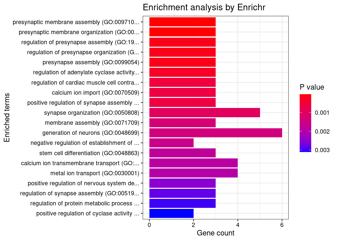
| Version | Author | Date |
|---|---|---|
| 9e83da3 | wesleycrouse | 2022-07-25 |
save(enrich_results, file="output/Prioritized_SCZ_genes_enrichment.RData")
write.csv(enrich_results, file="output/Prioritized_SCZ_genes_enrichment.csv")

enrich_results <- read.table("output/Prioritized_SCZ_genes_enrichment.csv", header=T, sep=",")

#report number of known IBD genes in annotations
length(known_genes)
[1] 120Summary table for selected tissue groups
#mapping genename to ensembl
genename_mapping <- data.frame(genename=as.character(), ensembl_id=as.character(), weight=as.character())

for (i in 1:length(results_dirs)){
  results_dir <- results_dirs[i]
  weight <- rev(unlist(strsplit(results_dir, "/")))[1]
  analysis_id <- paste(trait_id, weight, sep="_")

  sqlite <- RSQLite::dbDriver("SQLite")
  db = RSQLite::dbConnect(sqlite, paste0("/project2/mstephens/wcrouse/predictdb_nolnc/mashr_", weight, "_nolnc.db"))
  query <- function(...) RSQLite::dbGetQuery(db, ...)
  gene_info <- query("select gene, genename, gene_type from extra")
  RSQLite::dbDisconnect(db)

  genename_mapping <- rbind(genename_mapping, cbind(gene_info[,c("gene","genename")],weight))
}

genename_mapping <- genename_mapping[,c("gene","genename"),drop=F]
genename_mapping <- genename_mapping[!duplicated(genename_mapping),]
selected_groups <- c("CNS")
selected_genes <- unique(unlist(sapply(df_group[selected_groups], function(x){x$ctwas})))
weight_groups <- weight_groups[order(weight_groups$group),]
selected_weights <- weight_groups$weight[weight_groups$group %in% selected_groups]
gene_pips_by_weight <- gene_pips_by_weight_bkup
results_table <- as.data.frame(round(gene_pips_by_weight[selected_genes,selected_weights],3))
results_table$n_discovered <- apply(results_table>0.8,1,sum,na.rm=T)
results_table$n_imputed <- apply(results_table, 1, function(x){sum(!is.na(x))-1})
results_table$ensembl_gene_id <- genename_mapping$gene[sapply(rownames(results_table), match, table=genename_mapping$genename)]
results_table$ensembl_gene_id <- sapply(results_table$ensembl_gene_id, function(x){unlist(strsplit(x, "[.]"))[1]})
results_table <- cbind(results_table, G_list[sapply(results_table$ensembl_gene_id, match, table=G_list$ensembl_gene_id),c("chromosome_name","start_position","end_position","nearby","nearest","distance","which_nearest")])
results_table$known <- rownames(results_table) %in% known_genes
load(paste0("group_enrichment_results_", trait_id, ".RData"))
group_enrichment_results$group <- as.character(group_enrichment_results$group)
group_enrichment_results$db <- as.character(group_enrichment_results$db)
group_enrichment_results <- group_enrichment_results[group_enrichment_results$group %in% selected_groups,,drop=F]
results_table$enriched_terms <- sapply(rownames(results_table), function(x){paste(group_enrichment_results$Term[grep(x, group_enrichment_results$Genes)],collapse="; ")})
write.csv(results_table, file=paste0("summary_table_SCZ_nolnc_corrected.csv"))Results and figures for the paper
Gene expression explains a small proportion of heritability
These MESC results use matching summary statistics and GTEx v8 models provided by MESC.
library(ggrepel)

mesc_results <- as.data.frame(data.table::fread("output/allweight_heritability.txt"))

mesc_results <- mesc_results[mesc_results$trait==trait_id,]

mesc_results$`h2med/h2g` <- mesc_results$h2med/mesc_results$h2
mesc_results$weight[!is.na(mesc_results$weight_predictdb)] <- mesc_results$weight_predictdb[!is.na(mesc_results$weight_predictdb)]
mesc_results <- mesc_results[,colnames(mesc_results)!="weight_predictdb"]
rownames(mesc_results) <- mesc_results$weight

output$pve_med <- output$pve_g / (output$pve_g + output$pve_s)
rownames(output) <- output$weight

df_plot <- output
df_plot <- df_plot[mesc_results$weight,]
df_plot$mesc <- as.numeric(mesc_results$`h2med/h2g`)
df_plot$ctwas <- as.numeric(df_plot$pve_med)
df_plot$tissue <- as.character(sapply(df_plot$weight, function(x){paste(unlist(strsplit(x, "_")), collapse=" ")}))

df_plot$label <- ""
label_list <- c("Artery Aorta", "Brain Hypothalamus")

df_plot$label[df_plot$tissue %in% label_list] <- df_plot$tissue[df_plot$tissue %in% label_list]

####################

pdf(file = "output/SCZ_cTWAS_vs_MESC.pdf", width = 4, height = 3)

p <- ggplot(df_plot, aes(mesc, ctwas, label = label)) + geom_point(color = "blue", size=1.5)
p <- p + geom_text_repel(size=3,
                         max.time=20,
                         max.iter=400000,
                         seed=1,
                         max.overlaps=Inf,
                         #force=2.8,
                         #force_pull=0.3,
                         force=1,
                         force_pull=1,
                         min.segment.length=0)
p <- p + ylab("(Gene PVE) / (Total PVE) using cTWAS") + xlab("(h2med) / (h2g) using MESC")
p <- p + geom_abline(slope=1, intercept=0, linetype=3, alpha=0.4)

xy_min <- min(df_plot$mesc, df_plot$ctwas, na.rm=T)
xy_max <- max(df_plot$mesc, df_plot$ctwas, na.rm=T)

p <- p + xlim(xy_min,xy_max) + ylim(xy_min,xy_max)

fit <- lm(ctwas~0+mesc, data=df_plot)
p <- p + geom_abline(slope=summary(fit)$coefficients["mesc","Estimate"], intercept=0, linetype=2, color="blue", alpha=0.4)

p <- p + theme_bw()


p <- p + theme(axis.title = element_text(color = "grey20", size = 10)) + ggtitle("SCZ")

p
Warning: Removed 1 rows containing missing values (geom_point).Warning: Removed 1 rows containing missing values (geom_text_repel).dev.off()png
2 pWarning: Removed 1 rows containing missing values (geom_point).
Warning: Removed 1 rows containing missing values (geom_text_repel).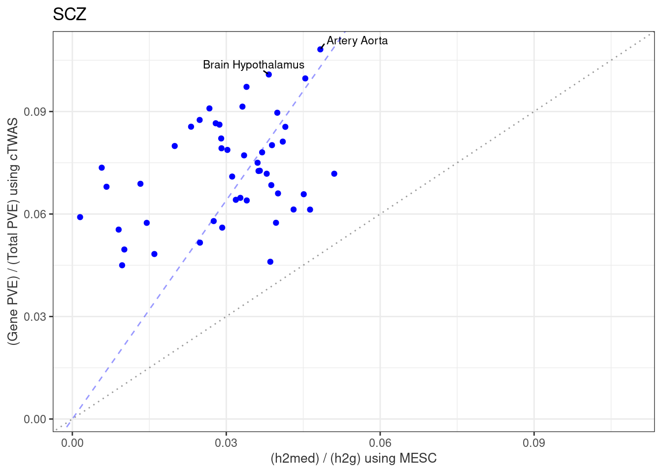
| Version | Author | Date |
|---|---|---|
| 2af4567 | wesleycrouse | 2022-09-02 |
| 0b519f1 | wesleycrouse | 2022-07-28 |
| c19144f | wesleycrouse | 2022-07-28 |
| 0f5b69a | wesleycrouse | 2022-07-28 |
| cb3f976 | wesleycrouse | 2022-07-27 |
| dd9f346 | wesleycrouse | 2022-07-27 |
| 7474fef | wesleycrouse | 2022-07-26 |
| 9ad1d4f | wesleycrouse | 2022-07-26 |
| d34b3a0 | wesleycrouse | 2022-07-19 |
####################

df_plot$tissue_number <- order(df_plot$weight)

df_plot$legend_entry <- sapply(1:nrow(df_plot), function(x){paste0(df_plot$tissue_number[x], ": ", df_plot$tissue[x])})


png(filename = "output/SCZ_cTWAS_vs_MESC_v2.png", width = 6, height = 5, units = "in", res=150)

p <- ggplot(df_plot, aes(mesc, ctwas, label = tissue_number))

p <- p + geom_point(color = "blue", size=1.5)

p <- p + geom_text_repel(min.segment.length=0,
                         size=2.4,
                         seed=1,
                         max.overlaps=Inf,
                         force=2,
                         force_pull=0.5)
p <- p + ylab("(Gene PVE) / (Total PVE) using cTWAS") + xlab("(h2med) / (h2g) using MESC")

p <- p + geom_abline(slope=1, intercept=0, linetype=3, alpha=0.4)

xy_min <- min(df_plot$mesc, df_plot$ctwas, na.rm=T)
xy_max <- max(df_plot$mesc, df_plot$ctwas, na.rm=T)

p <- p + xlim(xy_min,xy_max) + ylim(xy_min,xy_max)

fit <- lm(ctwas~0+mesc, data=df_plot)
p <- p + geom_abline(slope=summary(fit)$coefficients["mesc","Estimate"], intercept=0, linetype=2, color="blue", alpha=0.4)

p <- p + theme_bw()

#p <- p + theme(plot.margin = unit(c(1,15,1,1), "lines"))
# y_values <- xy_max-(xy_max-xy_min)*(1:nrow(df_plot))/nrow(df_plot)
# p <- p + geom_text(aes(label=legend_entry, x=xy_max, y=y_values, hjust=0))

p
Warning: Removed 1 rows containing missing values (geom_point).
Warning: Removed 1 rows containing missing values (geom_text_repel).dev.off()png
2 pWarning: Removed 1 rows containing missing values (geom_point).
Warning: Removed 1 rows containing missing values (geom_text_repel).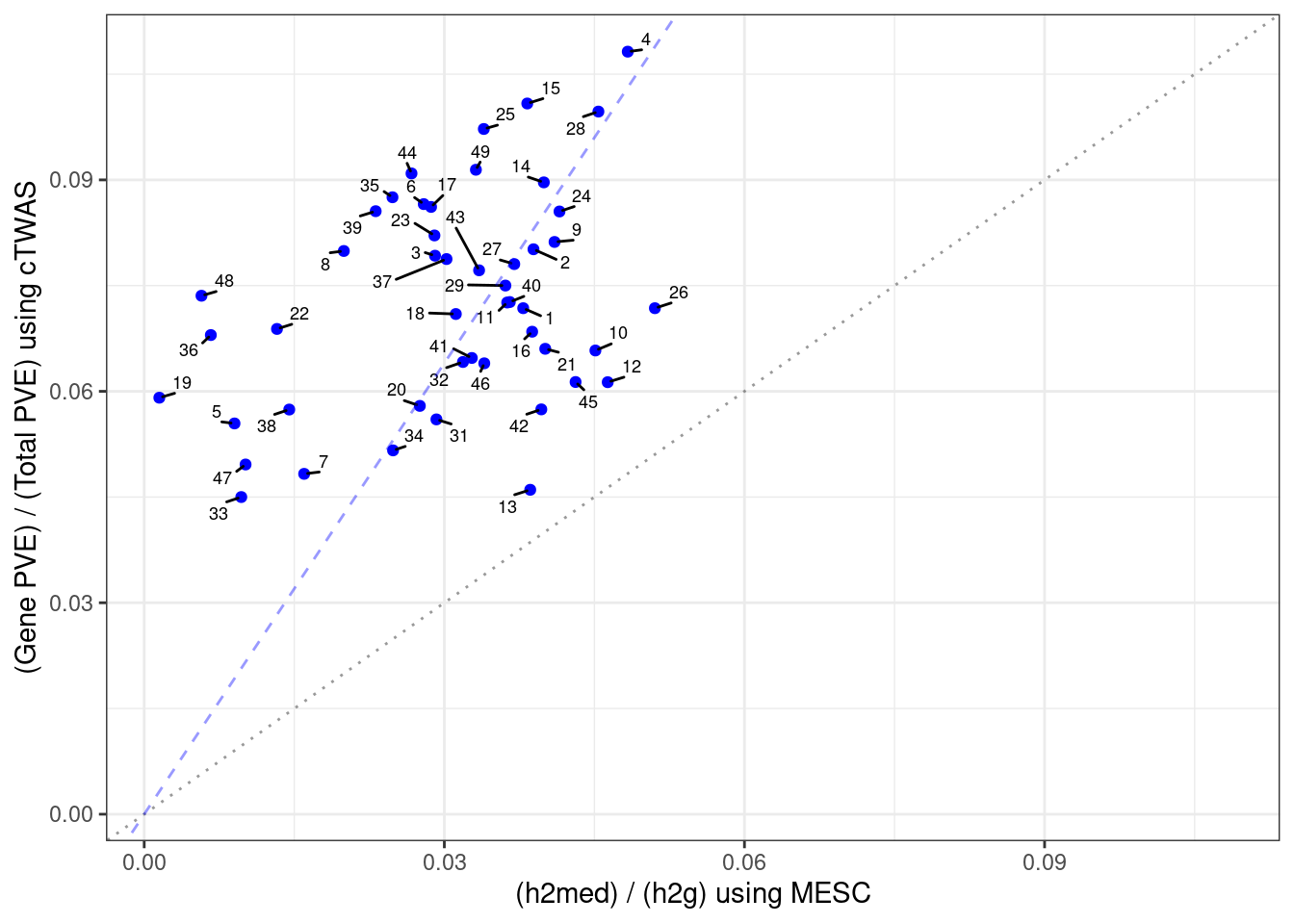
| Version | Author | Date |
|---|---|---|
| 7526db7 | wesleycrouse | 2022-10-03 |
| eb3c5bf | wesleycrouse | 2022-09-27 |
| 3349d12 | wesleycrouse | 2022-09-16 |
| 6a57156 | wesleycrouse | 2022-09-14 |
| 220ba1d | wesleycrouse | 2022-09-09 |
| 2af4567 | wesleycrouse | 2022-09-02 |
| 0b519f1 | wesleycrouse | 2022-07-28 |
| c19144f | wesleycrouse | 2022-07-28 |
| 0f5b69a | wesleycrouse | 2022-07-28 |
| cb3f976 | wesleycrouse | 2022-07-27 |
| dd9f346 | wesleycrouse | 2022-07-27 |
| 7474fef | wesleycrouse | 2022-07-26 |
| 9ad1d4f | wesleycrouse | 2022-07-26 |
| d34b3a0 | wesleycrouse | 2022-07-19 |
####################

#report correlation between cTWAS and MESC
cor(df_plot$mesc, df_plot$ctwas, use="complete.obs")
[1] 0.3782199cTWAS finds fewer genes than TWAS
library(ggrepel)

df_plot <- output
#df_plot <- df_plot[selected_weights,,drop=F]
df_plot$tissue <- sapply(df_plot$weight, function(x){paste(unlist(strsplit(x,"_")),collapse=" ")})

png(filename = "output/SCZ_cTWAS_vs_TWAS_all.png", width = 6, height = 5, units = "in", res=150)

p <- ggplot(df_plot, aes(n_twas, n_ctwas, label = tissue))
p <- p + geom_point(color = "blue", size=1.5)
p <- p + geom_text_repel(min.segment.length=0,
                         size=2.4,
                         seed=1,
                         max.overlaps=Inf,
                         force=2,
                         force_pull=0.5)
p <- p + ylab("Number of cTWAS genes") + xlab("Number of TWAS genes")
p <- p + scale_y_continuous(breaks=seq(0,max(df_plot$n_ctwas),2))
p <- p + scale_x_continuous(breaks=seq(0,max(df_plot$n_twas),5))
p <- p + theme_bw()

fit <- lm(n_ctwas~0+n_twas, data=df_plot)
p <- p + geom_abline(slope=summary(fit)$coefficients["n_twas","Estimate"], intercept=0, linetype=2, color="blue")

p

dev.off()
png
2 p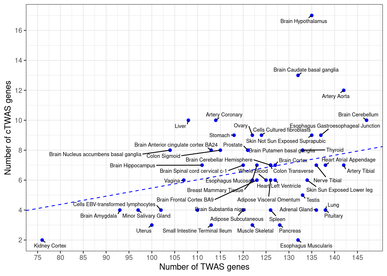
| Version | Author | Date |
|---|---|---|
| 7526db7 | wesleycrouse | 2022-10-03 |
| eb3c5bf | wesleycrouse | 2022-09-27 |
| 3349d12 | wesleycrouse | 2022-09-16 |
| 6a57156 | wesleycrouse | 2022-09-14 |
| 220ba1d | wesleycrouse | 2022-09-09 |
| 2af4567 | wesleycrouse | 2022-09-02 |
| 0b519f1 | wesleycrouse | 2022-07-28 |
| c19144f | wesleycrouse | 2022-07-28 |
| 0f5b69a | wesleycrouse | 2022-07-28 |
| cb3f976 | wesleycrouse | 2022-07-27 |
| dd9f346 | wesleycrouse | 2022-07-27 |
| 7474fef | wesleycrouse | 2022-07-26 |
| 9ad1d4f | wesleycrouse | 2022-07-26 |
| f2cc313 | wesleycrouse | 2022-07-25 |
| 9e83da3 | wesleycrouse | 2022-07-25 |
| 4ded2ef | wesleycrouse | 2022-07-19 |
#report correlation between cTWAS and TWAS
cor(df_plot$n_ctwas, df_plot$n_twas)
[1] 0.3468328####################
#using cutpoint for number of ctwas and twas genes to determine which tissues to label
df_plot <- output
df_plot$tissue <- sapply(df_plot$weight, function(x){paste(unlist(strsplit(x,"_")),collapse=" ")})
df_plot$tissue[df_plot$n_ctwas < 11.5 & df_plot$n_twas < 135] <- ""
png(filename = "output/SCZ_cTWAS_vs_TWAS_top.png", width = 6, height = 5, units = "in", res=150)
p <- ggplot(df_plot, aes(n_twas, n_ctwas, label = tissue))
p <- p + geom_point(color = "blue", size=1.5)
p <- p + geom_text_repel(min.segment.length=0,
size=2.4,
seed=1,
max.overlaps=Inf,
force=1,
force_pull=0.5)
p <- p + ylab("Number of cTWAS genes") + xlab("Number of TWAS genes")
p <- p + scale_y_continuous(breaks=seq(0,max(df_plot$n_ctwas),2))
p <- p + scale_x_continuous(breaks=seq(0,max(df_plot$n_twas),5))
p <- p + theme_bw()
fit <- lm(n_ctwas~0+n_twas, data=df_plot)
p <- p + geom_abline(slope=summary(fit)$coefficients["n_twas","Estimate"], intercept=0, linetype=2, color="blue")
p
dev.off()png
2 p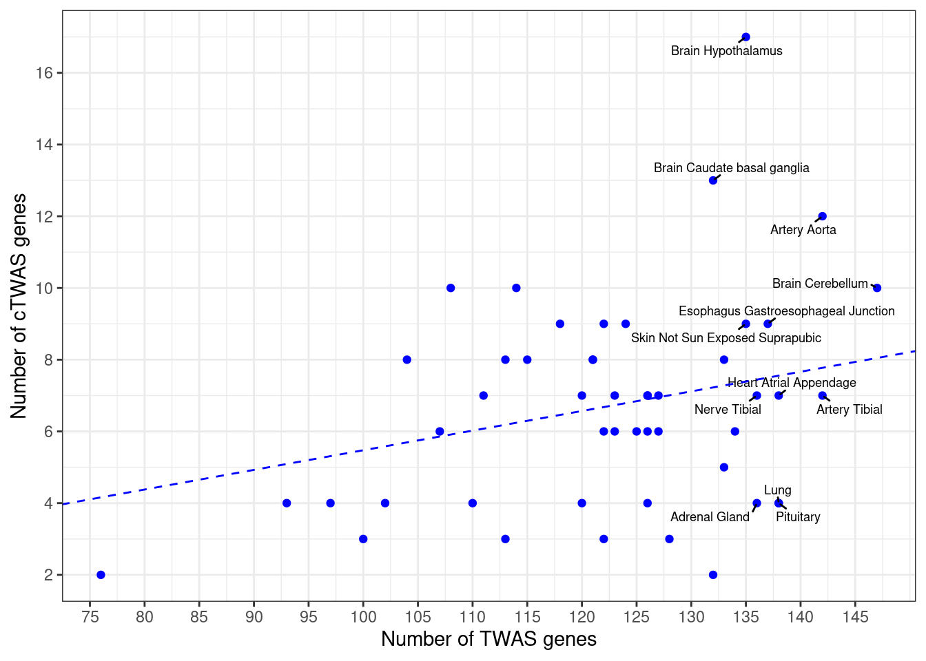
####################
#only labeling genes in selected tissue groups

df_plot <- output
df_plot$tissue <- sapply(df_plot$weight, function(x){paste(unlist(strsplit(x,"_")),collapse=" ")})

df_plot[!(df_plot$weight %in% selected_weights),"tissue"] <- ""

png(filename = "output/SCZ_cTWAS_vs_TWAS_selected.png", width = 6, height = 5, units = "in", res=150)

p <- ggplot(df_plot, aes(n_twas, n_ctwas, label = tissue))
p <- p + geom_point(color = "blue", size=1.5)
p <- p + geom_text_repel(min.segment.length=0,
                         size=2.4,
                         seed=1,
                         max.overlaps=Inf,
                         force=1,
                         force_pull=0.5)
p <- p + ylab("Number of cTWAS genes") + xlab("Number of TWAS genes")
p <- p + scale_y_continuous(breaks=seq(0,max(df_plot$n_ctwas),2))
p <- p + scale_x_continuous(breaks=seq(0,max(df_plot$n_twas),5))
p <- p + theme_bw()

fit <- lm(n_ctwas~0+n_twas, data=df_plot)
p <- p + geom_abline(slope=summary(fit)$coefficients["n_twas","Estimate"], intercept=0, linetype=2, color="blue")

p

dev.off()
png
2 p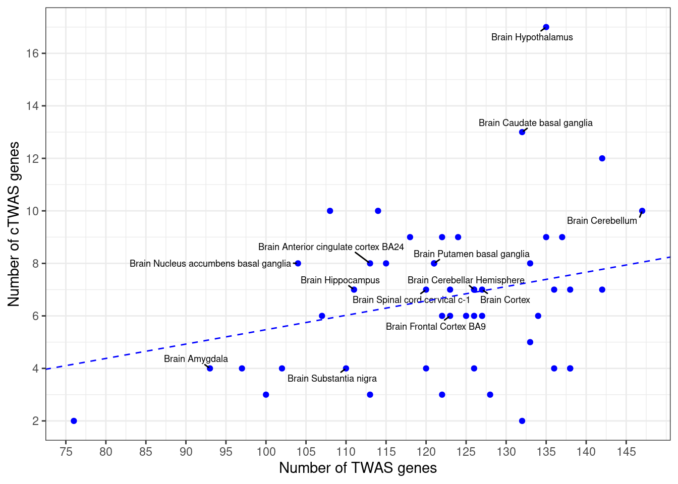
####################
#minimum and maximum number of discoveries per tissues
min(output$n_ctwas)
[1] 2max(output$n_ctwas)[1] 17min(output$n_twas)[1] 76max(output$n_twas)[1] 147####################
df_plot <- output
df_plot$tissue <- sapply(df_plot$weight, function(x){paste(unlist(strsplit(x,"_")),collapse=" ")})
df_plot$label <- ""
#label_list <- c("Artery Aorta", "Brain Hypothalamus")
label_list <- c(df_plot$tissue[which.max(df_plot$n_twas)], df_plot$tissue[which.max(df_plot$n_ctwas)])
df_plot$label[df_plot$tissue %in% label_list] <- df_plot$tissue[df_plot$tissue %in% label_list]
pdf(file = "output/SCZ_cTWAS_vs_TWAS.pdf", width = 4, height = 3)
p <- ggplot(df_plot, aes(n_twas, n_ctwas, label = label))
p <- p + geom_point(color = "blue", size=1.5)
p <- p + geom_text_repel(min.segment.length=0,
size=3,
seed=1,
max.overlaps=Inf,
force=1,
force_pull=1)
p <- p + ylab("Number of cTWAS Genes") + xlab("Number of TWAS Genes")
p <- p + scale_y_continuous(breaks=seq(0,max(df_plot$n_ctwas),2))
p <- p + scale_x_continuous(breaks=seq(0,max(df_plot$n_twas),10))
p <- p + theme_bw()
fit <- lm(n_ctwas~0+n_twas, data=df_plot)
p <- p + geom_abline(slope=summary(fit)$coefficients["n_twas","Estimate"], intercept=0, linetype=2, color="blue", alpha=0.4) + ggtitle("SCZ")
p
dev.off()png
2 Most cTWAS genes were found in a small number of tissues
#number of tissues with PIP>0.5 for cTWAS genes
gene_pips_by_weight_bkup <- gene_pips_by_weight
gene_pips_by_weight[is.na(gene_pips_by_weight)] <- 0

gene_pips_by_weight <- gene_pips_by_weight[apply(gene_pips_by_weight[,selected_weights,drop=F],1,max)>0.8,,drop=F]

ctwas_frequency <- rowSums(gene_pips_by_weight>0.5)
hist(ctwas_frequency, col="grey", breaks=0:max(ctwas_frequency), xlim=c(0,max(ctwas_frequency)),
     xlab="Number of Tissues with PIP>0.5",
     ylab="Number of cTWAS Genes",
     main="")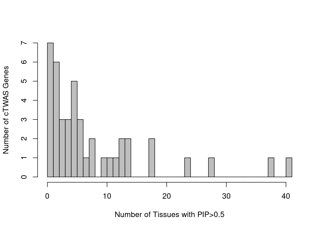
#report number of genes in each tissue bin
table(ctwas_frequency)
ctwas_frequency
1 2 3 4 5 6 7 8 10 11 12 13 14 18 24 28 38 41
7 6 3 3 5 3 1 2 1 1 1 2 2 2 1 1 1 1 #% less than 5
sum(ctwas_frequency<5)/length(ctwas_frequency)[1] 0.4418605#% equal to 1
sum(ctwas_frequency==1)/length(ctwas_frequency)[1] 0.1627907#list the frequency for each gene
ctwas_frequencyHIST1H2BN BHLHE41 SF3B1 ZNF823 VRK2 DRD2 FANCI ELAC2 IRF3 CAAP1 B3GAT1 PDXDC1 SPECC1 FURIN PPP1R13B TMEM222 JSRP1 SYTL1 TMEM81 PACSIN3 TBC1D29 WBP2 ZCCHC2 KCNG1 GALNT2 FEZF1 LRP8 MAP3K11 SSPN NPIPA1 TNFRSF13C SPCS1 PTPA CCDC6 PCBP2 RCBTB1 FOXO6 C19orf35 VPS8 GAL PPP1R16B TMEM56 ZNF844
28 18 38 41 24 2 13 13 14 5 4 3 8 12 10 18 1 14 1 5 6 6 3 2 2 4 2 8 1 2 2 1 11 1 6 5 4 3 5 1 7 5 1 Many cTWAS genes are novel - selected tissues
“Novel” is defined as 1) not in the silver standard, and 2) not the gene nearest to a genome-wide significant GWAS peak
#barplot of number of cTWAS genes in each tissue
df_plot <- output[output$weight %in% selected_weights,,drop=F]
df_plot <- df_plot[order(-df_plot$n_ctwas),,drop=F]

df_plot$tissue <- sapply(df_plot$weight, function(x){paste(unlist(strsplit(x,"_")),collapse=" ")})

pdf(file = "output/SCZ_novel_ctwas_genes.pdf", width = 2.75, height = 3)

par(mar=c(6.6, 3.6, 1.1, 0.6))

barplot(df_plot$n_ctwas, names.arg=df_plot$tissue, las=2, ylab="Number of cTWAS Genes", main="",
        cex.lab=0.7,
        cex.axis=0.7,
        cex.names=0.6,
        axis.lty=1)


results_table$novel <- !(results_table$nearest | results_table$known)
df_plot$n_novel <- sapply(df_plot$weight, function(x){sum(results_table[df[[x]]$ctwas,"novel"], na.rm=T)})

barplot(df_plot$n_novel, names.arg=df_plot$tissue, las=2, col="blue", add=T, xaxt='n', yaxt='n')

legend("topright",
       legend = c("Silver Standard or\nNearest to GWAS Peak", "Novel"),
       fill = c("grey", "blue"), cex=0.6)

dev.off()
png
2 Number of cTWAS Genes - all tissues
df_plot <- output
df_plot <- df_plot[order(df_plot$n_ctwas),,drop=F]

df_plot$tissue <- sapply(df_plot$weight, function(x){paste(unlist(strsplit(x,"_")),collapse=" ")})

pdf(file = "output/SCZ_number_ctwas_genes.pdf", width = 7, height = 5)

par(mar=c(3.6, 8.6, 0.6, 1.6))

barplot(df_plot$n_ctwas, names.arg=df_plot$tissue, las=2, xlab="Number of cTWAS Genes", main="",
        cex.lab=0.8,
        cex.axis=0.8,
        cex.names=0.5,
        axis.lty=1,
        col=c("darkblue", "grey50"),
        horiz=T,
        las=1)

grid(nx = NULL,
     ny = NA,
     lty = 2, col = "grey", lwd = 1)

dev.off()
png
2 Summary table of results
selected_weights_whitespace <- sapply(selected_weights, function(x){paste(unlist(strsplit(x, "_")), collapse=" ")})

results_summary <- data.frame(genename=as.character(rownames(results_table)),
                              ensembl_gene_id=results_table$ensembl_gene_id,
                              gene_biotype=G_list$gene_biotype[sapply(results_table$ensembl_gene_id, match, table=G_list$ensembl_gene_id)],
                              chromosome=results_table$chromosome_name,
                              start_position=results_table$start_position,
                              max_pip_tissue=selected_weights_whitespace[apply(results_table[,selected_weights], 1, which.max)],
                              max_pip=apply(results_table[,selected_weights], 1, max, na.rm=T),
                              other_tissues_detected=apply(results_table[,selected_weights],1,function(x){paste(selected_weights_whitespace[which(x>0.8 & x!=max(x,na.rm=T))], collapse="; ")}),
                              nearby=results_table$nearby,
                              nearest=results_table$nearest,
                              distance=G_list$distance[sapply(results_table$ensembl_gene_id, match, table=G_list$ensembl_gene_id)],
                              known=results_table$known,
                              enriched_terms=results_table$enriched_terms)

results_summary <- results_summary[order(results_summary$chromosome, results_summary$start_position),]

write.csv(results_summary, file=paste0("results_summary_SCZ_nolnc_corrected.csv"))
GO enrichment for genes in selected tissues
#enrichment for cTWAS genes using enrichR
library(enrichR)

dbs <- c("GO_Biological_Process_2021")

GO_enrichment <- enrichr(selected_genes, dbs)
Uploading data to Enrichr... Warning in enrichr(selected_genes, dbs): genes must be a non-empty vector of gene names or a data.frame with genes and score.Done.
Querying GO_Biological_Process_2021... Done.
Parsing results... Done.for (db in dbs){
cat(paste0(db, "\n\n"))
enrich_results <- GO_enrichment[[db]]
enrich_results <- enrich_results[enrich_results$Adjusted.P.value<0.05,c("Term", "Overlap", "Adjusted.P.value", "Genes"),drop=F]
print(enrich_results)
print(plotEnrich(GO_enrichment[[db]]))
}GO_Biological_Process_2021
Term Overlap Adjusted.P.value Genes
1 presynaptic membrane assembly (GO:0097105) 3/10 0.01429521 PTPRD;NLGN4X;IL1RAPL1
2 presynaptic membrane organization (GO:0097090) 3/11 0.01429521 PTPRD;NLGN4X;IL1RAPL1
3 regulation of presynapse assembly (GO:1905606) 3/18 0.02742401 PTPRD;IL1RAPL1;LRRC4B
4 regulation of presynapse organization (GO:0099174) 3/18 0.02742401 PTPRD;IL1RAPL1;LRRC4B
5 presynapse assembly (GO:0099054) 3/18 0.02742401 PTPRD;NLGN4X;IL1RAPL1
6 regulation of adenylate cyclase activity (GO:0045761) 3/22 0.04238137 GABBR2;CACNA1C;CRHR1
| Version | Author | Date |
|---|---|---|
| 220ba1d | wesleycrouse | 2022-09-09 |
Summary table of results - version 2
results_summary <- data.frame(genename=as.character(rownames(results_table)),
                              ensembl_gene_id=results_table$ensembl_gene_id,
                              chromosome=results_table$chromosome_name,
                              start_position=results_table$start_position,
                              max_pip_tissue=selected_weights_whitespace[apply(results_table[,selected_weights], 1, which.max)],
                              max_pip_tissue_nospace=selected_weights[apply(results_table[,selected_weights], 1, which.max)],
                              max_pip=apply(results_table[,selected_weights], 1, max, na.rm=T),
                              other_tissues_detected=apply(results_table[,selected_weights],1,function(x){paste(selected_weights_whitespace[which(x>0.8 & x!=max(x,na.rm=T))], collapse="; ")}),
                              region_tag_tissue=NA,
                              z_tissue=NA,
                              num_eqtl_tissue=NA,
                              twas_fp_tissue=NA,
                              gene_nearest_region_peak_tissue=NA,
                              nearby=results_table$nearby,
                              nearest=results_table$nearest,
                              distance=results_table$distance,
                              which_nearest=results_table$which_nearest,
                              known=results_table$known,
                              stringsAsFactors=F)

for (i in 1:nrow(results_summary)){
  tissue <- results_summary$max_pip_tissue_nospace[i]
  gene <- results_summary$genename[i]
  gene_pips <- df[[tissue]]$gene_pips
  results_summary[i,c("region_tag_tissue", "z_tissue", "num_eqtl_tissue")] <- gene_pips[gene_pips$genename==gene,c("region_tag", "z", "num_eqtl")]
  region_tag <- results_summary$region_tag_tissue[i]
  results_summary$twas_fp_tissue[i] <- any(gene_pips$genename[gene_pips$region_tag==region_tag & gene_pips$genename!=gene] %in% df[[tissue]]$twas)


  region_pips <- df[[tissue]]$region_pips
  lead_snp <- region_pips$which_snp_maxz[region_pips$region==region_tag]

  chromosome <- z_snp$chrom[z_snp$id==lead_snp]
  lead_position <- z_snp$pos[z_snp$id==lead_snp]

  G_list_index <- which(G_list$chromosome_name==chromosome)

  distances <- sapply(G_list_index, function(i){
    if (lead_position >= G_list$start_position[i] & lead_position <= G_list$end_position[i]){
      distance <- 0
    } else {
      distance <- min(abs(G_list$start_position[i] - lead_position), abs(G_list$end_position[i] - lead_position))
    }
    distance
  })

  results_summary$gene_nearest_region_peak_tissue[i] <- paste0(G_list$hgnc_symbol[G_list_index[which(distances==min(distances))]], collapse="; ")

}

####################
#get positions for genes that are included in analysis but not protein coding, so not included in nearby/nearest analysis

G_list_bkup <- G_list

load(paste0("G_list_", trait_id, ".RData"))

indices <- which(is.na(results_summary$start_position))

for (i in indices){
  G_list_index <- which(results_summary$ensembl_gene_id[i]==G_list$ensembl_gene_id)
  results_summary$chromosome[i] <- G_list$chromosome_name[G_list_index]
  results_summary$start_position[i] <- G_list$start_position[G_list_index]
}

G_list <- G_list_bkup
rm(G_list_bkup)

####################
#GO enrichment of cTWAS genes
# genes <- results_summary$genename
#
# dbs <- c("GO_Biological_Process_2021", "GO_Cellular_Component_2021", "GO_Molecular_Function_2021")
# GO_enrichment <- enrichr(genes, dbs)
#
# save(GO_enrichment, file=paste0(trait_id, "_enrichment_results.RData"))

####################
#enrichment of silver standard genes
genes <- known_genes

dbs <- c("GO_Biological_Process_2021", "GO_Cellular_Component_2021", "GO_Molecular_Function_2021")
GO_enrichment_silver_standard <- enrichr(genes, dbs)
Uploading data to Enrichr... Done.
Querying GO_Biological_Process_2021... Done.
Querying GO_Cellular_Component_2021... Done.
Querying GO_Molecular_Function_2021... Done.
Parsing results... Done.save(GO_enrichment_silver_standard, file=paste0(trait_id, "_silver_standard_enrichment_results.RData"))
####################
#report GO cTWAS
load(paste0(trait_id, "_enrichment_results.RData"))
GO_enrichment <- do.call(rbind, GO_enrichment)
GO_enrichment$db <- sapply(rownames(GO_enrichment), function(x){unlist(strsplit(x, split="[.]"))[1]})
rownames(GO_enrichment) <- NULL
GO_enrichment <- GO_enrichment[GO_enrichment$Adjusted.P.value < 0.05,]
GO_enrichment <- GO_enrichment[order(-GO_enrichment$Odds.Ratio),]
results_summary$GO <- sapply(results_summary$genename, function(x){terms <- GO_enrichment$Term[grep(x, GO_enrichment$Genes)];
if (length(terms)>0){terms <- terms[1:min(length(terms),5)]};
paste0(terms, collapse="; ")})
####################
#report GO silver standard
GO_silver_standard_sigthresh <- 0.1
load(paste0(trait_id, "_silver_standard_enrichment_results.RData"))
GO_enrichment_silver_standard <- do.call(rbind, GO_enrichment_silver_standard)
GO_enrichment_silver_standard$db <- sapply(rownames(GO_enrichment_silver_standard), function(x){unlist(strsplit(x, split="[.]"))[1]})
rownames(GO_enrichment_silver_standard) <- NULL
GO_enrichment_silver_standard <- GO_enrichment_silver_standard[order(GO_enrichment_silver_standard$Adjusted.P.value),]
write.csv(GO_enrichment_silver_standard, file=paste0("output/SCZ_silver_standard_enrichment_results.csv"))
GO_enrichment_silver_standard <- GO_enrichment_silver_standard[GO_enrichment_silver_standard$Adjusted.P.value < GO_silver_standard_sigthresh,]
GO_enrichment_silver_standard <- GO_enrichment_silver_standard[order(-GO_enrichment_silver_standard$Odds.Ratio),]
#reload GO cTWAS for GO crosswalk
load(paste0(trait_id, "_enrichment_results.RData"))
GO_enrichment <- do.call(rbind, GO_enrichment)
GO_enrichment$db <- sapply(rownames(GO_enrichment), function(x){unlist(strsplit(x, split="[.]"))[1]})
rownames(GO_enrichment) <- NULL
#overlap between sets
GO_enrichment <- GO_enrichment[GO_enrichment$Term %in% GO_enrichment_silver_standard$Term,,drop=F]
GO_enrichment_silver_standard <- GO_enrichment_silver_standard[GO_enrichment_silver_standard$Term %in% GO_enrichment$Term,,drop=F]
GO_enrichment <- GO_enrichment[match(GO_enrichment_silver_standard$Term, GO_enrichment$Term),]
results_summary$GO_silver <- sapply(results_summary$genename, function(x){terms <- GO_enrichment$Term[grep(x, GO_enrichment$Genes)];
if (length(terms)>0){terms <- terms[1:min(length(terms),5)]};
paste0(terms, collapse="; ")})
####################
#report FUMA
FUMA <- data.table::fread(paste0("/project2/xinhe/shengqian/cTWAS/cTWAS_analysis/data/FUMA_output/SCZ_2018/GS.txt"))
FUMA <- FUMA[FUMA$Category %in% c("GO_bp", "GO_cc", "GO_mf"),,drop=F]
FUMA <- FUMA[order(FUMA$p),]
write.csv(FUMA, file="output/SCZ_MAGMA.csv")
#reload GO cTWAS for GO crosswalk
load(paste0(trait_id, "_enrichment_results.RData"))
GO_enrichment <- do.call(rbind, GO_enrichment)
GO_enrichment$db <- sapply(rownames(GO_enrichment), function(x){unlist(strsplit(x, split="[.]"))[1]})
rownames(GO_enrichment) <- NULL
GO_enrichment$Term_FUMA <- sapply(GO_enrichment$Term, function(x){rev(rev(unlist(strsplit(x, split=" [(]GO")))[-1])})
GO_enrichment$Term_FUMA <- paste0("GO_", toupper(gsub(" ", "_", GO_enrichment$Term_FUMA)))
#overlap between sets
GO_enrichment <- GO_enrichment[GO_enrichment$Term_FUMA %in% FUMA$GeneSet,,drop=F]
FUMA <- FUMA[FUMA$GeneSet %in% GO_enrichment$Term_FUMA]
GO_enrichment <- GO_enrichment[match(FUMA$GeneSet, GO_enrichment$Term_FUMA),]
results_summary$GO_MAGMA <- sapply(results_summary$genename, function(x){terms <- GO_enrichment$Term[grep(x, GO_enrichment$Genes)];
if (length(terms)>0){terms <- terms[1:min(length(terms),5)]};
paste0(terms, collapse="; ")})
####################
#report FUMA + susieGO
# gsesusie <- as.data.frame(readxl::read_xlsx("gsesusie_enrichment.xlsx", sheet=trait_id))
# gsesusie$GeneSet <- paste0("(", gsesusie$GeneSet, ")")
#
# #reload GO cTWAS for GO crosswalk
# load(paste0(trait_id, "_enrichment_results.RData"))
# GO_enrichment <- do.call(rbind, GO_enrichment)
# GO_enrichment$db <- sapply(rownames(GO_enrichment), function(x){unlist(strsplit(x, split="[.]"))[1]})
# rownames(GO_enrichment) <- NULL
#
# GO_enrichment$GeneSet <- sapply(GO_enrichment$Term, function(x){rev(unlist(strsplit(x, " ")))[1]})
#
# #overlap between sets
# GO_enrichment <- GO_enrichment[GO_enrichment$GeneSet %in% gsesusie$GeneSet,,drop=F]
# gsesusie <- gsesusie[gsesusie$GeneSet %in% GO_enrichment$GeneSet,,drop=F]
# GO_enrichment <- GO_enrichment[match(gsesusie$GeneSet, GO_enrichment$GeneSet),]
#
# results_summary$GO_MAGMA_SuSiE <- sapply(results_summary$genename, function(x){terms <- GO_enrichment$Term[grep(x, GO_enrichment$Genes)];
# if (length(terms)>0){terms <- terms[1:min(length(terms),5)]};
# paste0(terms, collapse="; ")})
####################
results_summary <- results_summary[order(results_summary$chromosome, results_summary$start_position),]
results_summary <- results_summary[,!(colnames(results_summary) %in% c("max_pip_tissue_nospace"))]
write.csv(results_summary, file=paste0("results_summary_SCZ_nolnc_v2_corrected.csv"))
#number of genes in silver standard or at least one enriched term from GO silver standard
sum(results_summary$GO_silver!="" | results_summary$known)[1] 6#number of genes in silver standard or at least one enriched term from GO silver standard or GO MAGMA
sum(results_summary$GO_silver!="" | results_summary$GO_MAGMA!="" | results_summary$known)[1] 7#number of genes in silver standard or at least one enriched term from GO silver standard or GO MAGMA or GO cTWAS
#sum(results_summary$GO_silver!="" | results_summary$GO_MAGMA!="" | results_summary$known | results_summary$GO!="")Summary table of results - Compact version
results_summary_compact <- results_summary[results_summary$max_pip>0.9,]

results_summary_compact$evidence  <- ""
results_summary_compact$evidence[which(results_summary_compact$known==T & results_summary_compact$nearest==T)] <- "S,G"
results_summary_compact$evidence[which(results_summary_compact$known==T & results_summary_compact$nearest!=T)] <- "S"
results_summary_compact$evidence[which(results_summary_compact$known!=T & results_summary_compact$nearest==T)] <- "G"

results_summary_compact <- results_summary_compact[,c("genename", "max_pip_tissue", "max_pip", "other_tissues_detected", "evidence")]

write.csv(results_summary_compact, file=paste0("results_summary_SCZ_compact.csv"), row.names=F)
Novel Genes by Tissue Group
#barplot of number of cTWAS genes in each tissue
df_plot <- -sort(-sapply(groups[groups!="None"], function(x){length(df_group[[x]][["ctwas"]])}))

par(mar=c(10.1, 4.1, 4.1, 2.1))
barplot(df_plot, las=2, ylab="Number of cTWAS Genes", main="Number of cTWAS Genes by Tissue Group")

df_plot_novel <- rep(NA, length(df_plot))
names(df_plot_novel) <- names(df_plot)

for (i in 1:length(df_plot)){
  genename <- df_group[[names(df_plot)[i]]]$ctwas
  gene <- genename_mapping$gene[match(genename, genename_mapping$genename)]
  gene <- sapply(gene, function(x){unlist(strsplit(x, "[.]"))[1]})

  G_list_subset <- G_list[match(gene, G_list$ensembl_gene_id),]

  G_list_subset$known <- G_list_subset$hgnc_symbol %in% known_genes

  df_plot_novel[i] <- sum(!(G_list_subset$known | G_list_subset$nearest), na.rm=T)
}

barplot(df_plot_novel, las=2, col="blue", add=T, xaxt='n', yaxt='n')

legend("topright",
       legend = c("Silver Standard or\nNearest to GWAS Peak", "Novel"),
       fill = c("grey", "blue"))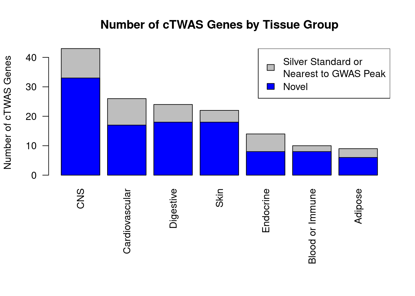
| Version | Author | Date |
|---|---|---|
| 220ba1d | wesleycrouse | 2022-09-09 |
##########

#barplot of number of cTWAS genes in each tissue
df_plot <- -sort(-sapply(groups[groups!="None"], function(x){length(df_group[[x]][["ctwas"]])}))

df_plot_novel <- rep(NA, length(df_plot))
names(df_plot_novel) <- names(df_plot)

for (i in 1:length(df_plot)){
  genename <- df_group[[names(df_plot)[i]]]$ctwas
  gene <- genename_mapping$gene[match(genename, genename_mapping$genename)]
  gene <- sapply(gene, function(x){unlist(strsplit(x, "[.]"))[1]})

  G_list_subset <- G_list[match(gene, G_list$ensembl_gene_id),]

  G_list_subset$known <- G_list_subset$hgnc_symbol %in% known_genes

  df_plot_novel[i] <- sum(!(G_list_subset$known | G_list_subset$nearest), na.rm=T)
}

pdf(file = "output/SCZ_novel_ctwas_genes_group.pdf", width = 2.75, height = 3)
par(mar=c(4.6, 3.6, 1.1, 0.6))

barplot(df_plot, las=2, col="blue", ylab="Number of cTWAS Genes", main="",
        cex.lab=0.8,
        cex.axis=0.8,
        cex.names=0.7,
        axis.lty=1)
barplot(df_plot-df_plot_novel, las=2, add=T, xaxt='n', yaxt='n')

legend("topright",
       legend = c("Silver Standard or\nNearest to GWAS Peak", "Novel"),
       fill = c("grey", "blue"), cex=0.5)

dev.off()
png
2 Updated locus plots
load(paste0("G_list_", trait_id, ".RData"))
G_list <- G_list[G_list$gene_biotype %in% c("protein_coding"),]
G_list$hgnc_symbol[G_list$hgnc_symbol==""] <- "-"
G_list$tss <- G_list[,c("end_position", "start_position")][cbind(1:nrow(G_list),G_list$strand/2+1.5)]

####################

locus_plot_final <- function(genename=NULL, tissue=NULL, xlim=NULL, return_table=F, label_panel="TWAS", label_genes=NULL, label_pos=NULL, plot_eqtl=NULL, draw_gene_track=T, legend_side="right"){
  results_dir <- results_dirs[grep(tissue, results_dirs)]
  weight <- rev(unlist(strsplit(results_dir, "/")))[1]
  weight <- unlist(strsplit(weight, split="_nolnc"))
  analysis_id <- paste(trait_id, weight, sep="_")

  #load ctwas results
  ctwas_res <- data.table::fread(paste0(results_dir, "/", analysis_id, "_ctwas.susieIrss.txt"))

  #make unique identifier for regions and effects
  ctwas_res$region_tag <- paste(ctwas_res$region_tag1, ctwas_res$region_tag2, sep="_")
  ctwas_res$region_cs_tag <- paste(ctwas_res$region_tag, ctwas_res$cs_index, sep="_")

  #load z scores for SNPs
  load(paste0(results_dir, "/", analysis_id, "_expr_z_snp.Rd"))

  #separate gene and SNP results
  ctwas_gene_res <- ctwas_res[ctwas_res$type == "gene", ]
  ctwas_gene_res <- data.frame(ctwas_gene_res)
  ctwas_snp_res <- ctwas_res[ctwas_res$type == "SNP", ]
  ctwas_snp_res <- data.frame(ctwas_snp_res)

  #add gene information to results
  sqlite <- RSQLite::dbDriver("SQLite")
  db = RSQLite::dbConnect(sqlite, paste0("/project2/mstephens/wcrouse/predictdb_nolnc/mashr_", weight, "_nolnc.db"))
  query <- function(...) RSQLite::dbGetQuery(db, ...)
  gene_info <- query("select gene, genename, gene_type from extra")
  RSQLite::dbDisconnect(db)

  ctwas_gene_res <- cbind(ctwas_gene_res, gene_info[sapply(ctwas_gene_res$id, match, gene_info$gene), c("genename", "gene_type")])

  #add z scores to results
  load(paste0(results_dir, "/", analysis_id, "_expr_z_gene.Rd"))
  ctwas_gene_res$z <- z_gene[ctwas_gene_res$id,]$z

  z_snp <- z_snp[z_snp$id %in% ctwas_snp_res$id,]
  ctwas_snp_res$z <- z_snp$z[match(ctwas_snp_res$id, z_snp$id)]

  #merge gene and snp results with added information
  ctwas_snp_res$genename=NA
  ctwas_snp_res$gene_type=NA

  ctwas_res <- rbind(ctwas_gene_res, ctwas_snp_res[,colnames(ctwas_gene_res)])

  region_tag <- ctwas_res$region_tag[which(ctwas_res$genename==genename)]

  region_tag1 <- unlist(strsplit(region_tag, "_"))[1]
  region_tag2 <- unlist(strsplit(region_tag, "_"))[2]

  a <- ctwas_res[ctwas_res$region_tag==region_tag,]

  rm(ctwas_res)

  regionlist <- readRDS(paste0(results_dir, "/", analysis_id, "_ctwas.regionlist.RDS"))
  region <- regionlist[[as.numeric(region_tag1)]][[region_tag2]]

  R_snp_info <- do.call(rbind, lapply(region$regRDS, function(x){data.table::fread(paste0(tools::file_path_sans_ext(x), ".Rvar"))}))

  a_pos_bkup <- a$pos
  a$pos[a$type=="gene"] <- G_list$tss[match(sapply(a$id[a$type=="gene"], function(x){unlist(strsplit(x, "[.]"))[1]}) ,G_list$ensembl_gene_id)]
  a$pos[is.na(a$pos)] <- a_pos_bkup[is.na(a$pos)]
  a$pos <- a$pos/1000000

  if (!is.null(xlim)){

    if (is.na(xlim[1])){
      xlim[1] <- min(a$pos)
    }

    if (is.na(xlim[2])){
      xlim[2] <- max(a$pos)
    }

    a <- a[a$pos>=xlim[1] & a$pos<=xlim[2],,drop=F]
  }

  focus <- genename

  if (is.null(label_genes)){
    label_genes <- focus
  }

  if (is.null(label_pos)){
    label_pos <- rep(3, length(label_genes))
  }

  if (is.null(plot_eqtl)){
    plot_eqtl <- focus
  }

  focus <- a$id[which(a$genename==focus)]
  a$focus <- 0
  a$focus <- as.numeric(a$id==focus)

  a$PVALUE <- (-log(2) - pnorm(abs(a$z), lower.tail=F, log.p=T))/log(10)

  R_gene <- readRDS(region$R_g_file)
  R_snp_gene <- readRDS(region$R_sg_file)
  R_snp <- as.matrix(Matrix::bdiag(lapply(region$regRDS, readRDS)))

  rownames(R_gene) <- region$gid
  colnames(R_gene) <- region$gid
  rownames(R_snp_gene) <- R_snp_info$id
  colnames(R_snp_gene) <- region$gid
  rownames(R_snp) <- R_snp_info$id
  colnames(R_snp) <- R_snp_info$id

  a$r2max <- NA
  a$r2max[a$type=="gene"] <- R_gene[focus,a$id[a$type=="gene"]]
  a$r2max[a$type=="SNP"] <- R_snp_gene[a$id[a$type=="SNP"],focus]

  r2cut <- 0.4
  colorsall <- c("#7fc97f", "#beaed4", "#fdc086")

  start <- min(a$pos)
  end <- max(a$pos)

  if (draw_gene_track){
    layout(matrix(1:4, ncol = 1), widths = 1, heights = c(1.5,0.25,1.5,0.75), respect = FALSE)
  } else {
    layout(matrix(1:3, ncol = 1), widths = 1, heights = c(1.5,0.25,1.5), respect = FALSE)
  }

  par(mar = c(0, 4.1, 0, 2.1))

  plot(a$pos[a$type=="SNP"], a$PVALUE[a$type == "SNP"], pch = 21, xlab=paste0("Chromosome ", region_tag1, " position (Mb)"), frame.plot=FALSE, bg = colorsall[1], ylab = "-log10(p value)", panel.first = grid(), ylim =c(0, max(a$PVALUE)*1.1), xaxt = 'n', xlim=c(start, end))

  points(a$pos[a$type=="SNP" & a$r2max > r2cut], a$PVALUE[a$type == "SNP"  & a$r2max > r2cut], pch = 21, bg = "purple")
  points(a$pos[a$type=="SNP" & a$focus == 1], a$PVALUE[a$type == "SNP" & a$focus == 1], pch = 21, bg = "salmon")
  points(a$pos[a$type=="gene"], a$PVALUE[a$type == "gene"], pch = 22, bg = colorsall[1], cex = 2)
  points(a$pos[a$type=="gene" & a$r2max > r2cut], a$PVALUE[a$type == "gene"  & a$r2max > r2cut], pch = 22, bg = "purple", cex = 2)
  points(a$pos[a$type=="gene" & a$focus == 1], a$PVALUE[a$type == "gene" & a$focus == 1], pch = 22, bg = "salmon", cex = 2)

  alpha=0.05
  abline(h=-log10(alpha/nrow(ctwas_gene_res)), col ="red", lty = 2)

  if (label_panel=="TWAS"){
    for (i in 1:length(label_genes)){
      text(a$pos[a$genename==label_genes[i]], a$PVALUE[a$genename==label_genes[i]], labels=label_genes[i], pos=label_pos[i], cex=0.7)
    }
  }

  par(mar = c(0.25, 4.1, 0.25, 2.1))

  plot(NA, xlim = c(start, end), ylim = c(0, length(plot_eqtl)), frame.plot = F, axes = F, xlab = NA, ylab = NA)

  for (i in 1:length(plot_eqtl)){
    cgene <- a$id[which(a$genename==plot_eqtl[i])]
    load(paste0(results_dir, "/",analysis_id, "_expr_chr", region_tag1, ".exprqc.Rd"))
    eqtls <- rownames(wgtlist[[cgene]])
    eqtl_pos <- a$pos[a$id %in% eqtls]

    col="grey"

    rect(start, length(plot_eqtl)+1-i-0.8, end, length(plot_eqtl)+1-i-0.2, col = col, border = T, lwd = 1)

    if (length(eqtl_pos)>0){
      for (j in 1:length(eqtl_pos)){
        segments(x0=eqtl_pos[j], x1=eqtl_pos[j], y0=length(plot_eqtl)+1-i-0.2, length(plot_eqtl)+1-i-0.8, lwd=1.5)
      }
    }
  }

  text(start, length(plot_eqtl)-(1:length(plot_eqtl))+0.5,
       labels = plot_eqtl, srt = 0, pos = 2, xpd = TRUE, cex=0.7)

  par(mar = c(4.1, 4.1, 0, 2.1))

  plot(a$pos[a$type=="SNP"], a$PVALUE[a$type == "SNP"], pch = 19, xlab=paste0("Chromosome ", region_tag1, " position (Mb)"),frame.plot=FALSE, col = "white", ylim= c(0,1.1), ylab = "cTWAS PIP", xlim = c(start, end))

  grid()
  points(a$pos[a$type=="SNP"], a$susie_pip[a$type == "SNP"], pch = 21, xlab="Genomic position", bg = colorsall[1])
  points(a$pos[a$type=="SNP" & a$r2max > r2cut], a$susie_pip[a$type == "SNP"  & a$r2max >r2cut], pch = 21, bg = "purple")
  points(a$pos[a$type=="SNP" & a$focus == 1], a$susie_pip[a$type == "SNP" & a$focus == 1], pch = 21, bg = "salmon")
  points(a$pos[a$type=="gene"], a$susie_pip[a$type == "gene"], pch = 22, bg = colorsall[1], cex = 2)
  points(a$pos[a$type=="gene" & a$r2max > r2cut], a$susie_pip[a$type == "gene"  & a$r2max > r2cut], pch = 22, bg = "purple", cex = 2)
  points(a$pos[a$type=="gene" & a$focus == 1], a$susie_pip[a$type == "gene" & a$focus == 1], pch = 22, bg = "salmon", cex = 2)

  x_pos <- ifelse(legend_side=="right", max(a$pos)-0.2*(max(a$pos)-min(a$pos)), min(a$pos)+0.05*(max(a$pos)-min(a$pos)))

  legend(x_pos, y= 1 ,c("Gene", "SNP","Lead TWAS Gene", "R2 > 0.4", "R2 <= 0.4"), pch = c(22,21,19,19,19), col = c("black", "black", "salmon", "purple", colorsall[1]), cex=0.7, title.adj = 0)

  if (label_panel=="cTWAS"){
    for (i in 1:length(label_genes)){
      text(a$pos[a$genename==label_genes[i]], a$susie_pip[a$genename==label_genes[i]], labels=label_genes[i], pos=label_pos[i], cex=0.7)
    }
  }

  if (draw_gene_track){
    source("code/trackplot.R")

    query_ucsc = TRUE
    build = "hg38"
    col = "gray70"
    txname = NULL
    genename = NULL
    collapse_txs = TRUE
    gene_model = "data/hg38.ensGene.gtf.gz"
    isGTF = T

    ##########
    start <- min(a$pos)*1000000
    end <- max(a$pos)*1000000
    chr <- paste0("chr",as.character(unique(a$chrom)))

    #collect gene models
    if(is.null(gene_model)){
      if(query_ucsc){
        message("Missing gene model. Trying to query UCSC genome browser..")
        etbl = .extract_geneModel_ucsc(chr, start = start, end = end, refBuild = build, txname = txname, genename = genename)
      } else{
        etbl = NULL
      }
    } else{
      if(isGTF){
        etbl = .parse_gtf(gtf = gene_model, chr = chr, start = start, end = end, txname = txname, genename = genename)
      } else{
        etbl = .extract_geneModel(ucsc_tbl = gene_model, chr = chr, start = start, end = end, txname = txname, genename = genename)
      }
    }

    #draw gene models
    if(!is.null(etbl)){
      if(collapse_txs){
        etbl = .collapse_tx(etbl)
      }

      #subset to protein coding genes in ensembl and lincRNAs included in the analysis
      #etbl <- etbl[names(etbl) %in% G_list$ensembl_gene_id]
      etbl <- etbl[names(etbl) %in% c(G_list$ensembl_gene_id[G_list$gene_biotype=="protein_coding"], sapply(a$id[a$type=="gene"], function(x){unlist(strsplit(x, split="[.]"))[1]}))]

      for (i in 1:length(etbl)){
        ensembl_name <- attr(etbl[[i]], "gene")
        gene_name <- G_list$hgnc_symbol[match(ensembl_name, G_list$ensembl_gene_id)]
        if (gene_name=="" | is.na(gene_name)){
          gene_name <- a$genename[sapply(a$id, function(x){unlist(strsplit(x,split="[.]"))[1]})==ensembl_name]
        }
        if (length(gene_name)>0){
          attr(etbl[[i]], "gene") <- gene_name
        }

        attr(etbl[[i]], "imputed") <- ensembl_name %in% sapply(ctwas_gene_res$id, function(x){unlist(strsplit(x, split="[.]"))[1]})

      }

      par(mar = c(0, 4.1, 0, 2.1))

      plot(NA, xlim = c(start, end), ylim = c(0, length(etbl)), frame.plot = FALSE, axes = FALSE, xlab = NA, ylab = NA)

      etbl <- etbl[order(-sapply(etbl, function(x){attr(x, "start")}))]

      for(tx_id in 1:length(etbl)){
        txtbl = etbl[[tx_id]]

        if (attr(txtbl, "imputed")){
          exon_col = "#192a56"
        } else {
          exon_col = "darkred"
        }

        segments(x0 = attr(txtbl, "start"), y0 = tx_id-0.45, x1 = attr(txtbl, "end"), y1 = tx_id-0.45, col = exon_col, lwd = 1)

        if(is.na(attr(txtbl, "tx"))){
          text(x = start, y = tx_id-0.45, labels = paste0(attr(txtbl, "gene")), cex = 0.7, adj = 0, srt = 0, pos = 2, xpd = TRUE)
        } else {
          text(x = start, y = tx_id-0.45, labels = paste0(attr(txtbl, "tx"), " [", attr(txtbl, "gene"), "]"), cex = 0.7, adj = 0, srt = 0, pos = 2, xpd = TRUE)
        }

        rect(xleft = txtbl[[1]], ybottom = tx_id-0.75, xright = txtbl[[2]], ytop = tx_id-0.25, col = exon_col, border = NA)
        if(attr(txtbl, "strand") == "+"){
          dirat = pretty(x = c(min(txtbl[[1]]), max(txtbl[[2]])))
          dirat[1] = min(txtbl[[1]]) #Avoid drawing arrows outside gene length
          dirat[length(dirat)] = max(txtbl[[2]])
          points(x = dirat, y = rep(tx_id-0.45, length(dirat)), pch = ">", col = exon_col)
        }else{
          dirat = pretty(x = c(min(txtbl[[1]]), max(txtbl[[2]])))
          dirat[1] = min(txtbl[[1]]) #Avoid drawing arrows outside gene length
          dirat[length(dirat)] = max(txtbl[[2]])
          points(x = dirat, y = rep(tx_id-0.45, length(dirat)), pch = "<", col = exon_col)
        }
      }
    }
  }

  if (return_table){
    return(a)
  }
}
sessionInfo()R version 3.6.1 (2019-07-05)
Platform: x86_64-pc-linux-gnu (64-bit)
Running under: Scientific Linux 7.4 (Nitrogen)
Matrix products: default
BLAS/LAPACK: /software/openblas-0.2.19-el7-x86_64/lib/libopenblas_haswellp-r0.2.19.so
locale:
[1] LC_CTYPE=en_US.UTF-8 LC_NUMERIC=C LC_TIME=en_US.UTF-8 LC_COLLATE=en_US.UTF-8 LC_MONETARY=en_US.UTF-8 LC_MESSAGES=en_US.UTF-8 LC_PAPER=en_US.UTF-8 LC_NAME=C LC_ADDRESS=C LC_TELEPHONE=C LC_MEASUREMENT=en_US.UTF-8 LC_IDENTIFICATION=C
attached base packages:
[1] stats graphics grDevices utils datasets methods base
other attached packages:
[1] ggrepel_0.9.1 ggplot2_3.3.5 WebGestaltR_0.4.4 enrichR_3.0
loaded via a namespace (and not attached):
[1] Rcpp_1.0.6 svglite_1.2.2 lattice_0.20-38 rprojroot_2.0.2 digest_0.6.20 foreach_1.5.1 utf8_1.2.1 cellranger_1.1.0 R6_2.5.0 RSQLite_2.2.7 evaluate_0.14 httr_1.4.1 pillar_1.7.0 gdtools_0.1.9 rlang_1.0.2 readxl_1.3.1 curl_3.3 data.table_1.14.0 blob_1.2.1 whisker_0.3-2 Matrix_1.2-18 rmarkdown_1.13 apcluster_1.4.8 labeling_0.3 readr_1.4.0 stringr_1.4.0 bit_4.0.4 igraph_1.2.4.1 munsell_0.5.0 compiler_3.6.1 httpuv_1.5.1 xfun_0.8 pkgconfig_2.0.3 htmltools_0.5.2 tidyselect_1.1.2 tibble_3.1.7 workflowr_1.6.2 codetools_0.2-16 fansi_0.5.0 crayon_1.4.1 dplyr_1.0.9 withr_2.4.1 later_0.8.0 grid_3.6.1 jsonlite_1.6 gtable_0.3.0 lifecycle_1.0.1 DBI_1.1.1 git2r_0.26.1 magrittr_2.0.3 scales_1.2.0 cachem_1.0.5 cli_3.3.0 stringi_1.4.3 farver_2.1.0
[56] fs_1.5.2 promises_1.0.1 doRNG_1.8.2 doParallel_1.0.16 ellipsis_0.3.2 generics_0.0.2 vctrs_0.4.1 rjson_0.2.20 iterators_1.0.13 tools_3.6.1 bit64_4.0.5 glue_1.6.2 purrr_0.3.4 hms_1.1.0 rngtools_1.5 parallel_3.6.1 fastmap_1.1.0 yaml_2.2.0 colorspace_1.4-1 memoise_2.0.0 knitr_1.23