multitrait_allweight_figures
wesleycrouse
2022-07-19
Last updated: 2022-09-16
Checks: 7 0
Knit directory: ctwas_applied/
This reproducible R Markdown analysis was created with workflowr (version 1.6.2). The Checks tab describes the reproducibility checks that were applied when the results were created. The Past versions tab lists the development history.
Great! Since the R Markdown file has been committed to the Git repository, you know the exact version of the code that produced these results.
Great job! The global environment was empty. Objects defined in the global environment can affect the analysis in your R Markdown file in unknown ways. For reproduciblity it’s best to always run the code in an empty environment.
The command set.seed(20210726) was run prior to running the code in the R Markdown file. Setting a seed ensures that any results that rely on randomness, e.g. subsampling or permutations, are reproducible.
Great job! Recording the operating system, R version, and package versions is critical for reproducibility.
Nice! There were no cached chunks for this analysis, so you can be confident that you successfully produced the results during this run.
Great job! Using relative paths to the files within your workflowr project makes it easier to run your code on other machines.
Great! You are using Git for version control. Tracking code development and connecting the code version to the results is critical for reproducibility.
The results in this page were generated with repository version 6a57156. See the Past versions tab to see a history of the changes made to the R Markdown and HTML files.
Note that you need to be careful to ensure that all relevant files for the analysis have been committed to Git prior to generating the results (you can use wflow_publish or wflow_git_commit). workflowr only checks the R Markdown file, but you know if there are other scripts or data files that it depends on. Below is the status of the Git repository when the results were generated:
Untracked files:
    Untracked:  VennDiagram2022-09-16_21-42-57.log
    Untracked:  VennDiagram2022-09-16_21-43-19.log
    Untracked:  data/IBD_webgestalt_FDR05/
    Untracked:  output/IBD_GO_Venn_v2.pdf
    Untracked:  output/IBD_GO_Venn_v3.pdf
    Untracked:  output/IBD_GO_webgestalt.csv
    Untracked:  output/LDL_results_silver_bystander.csv
    Untracked:  temp.regionlist.RDS
    Untracked:  temp.regions.txt
    Untracked:  temp.susieIrss.txt
    Untracked:  temp.temp.susieIrssres.Rd
    Untracked:  temp_LDR/
    Untracked:  temp_ld_R_chr1.txt
    Untracked:  temp_ld_R_chr10.txt
    Untracked:  temp_ld_R_chr11.txt
    Untracked:  temp_ld_R_chr12.txt
    Untracked:  temp_ld_R_chr13.txt
    Untracked:  temp_ld_R_chr14.txt
    Untracked:  temp_ld_R_chr15.txt
    Untracked:  temp_ld_R_chr16.txt
    Untracked:  temp_ld_R_chr17.txt
    Untracked:  temp_ld_R_chr18.txt
    Untracked:  temp_ld_R_chr19.txt
    Untracked:  temp_ld_R_chr2.txt
    Untracked:  temp_ld_R_chr20.txt
    Untracked:  temp_ld_R_chr21.txt
    Untracked:  temp_ld_R_chr22.txt
    Untracked:  temp_ld_R_chr3.txt
    Untracked:  temp_ld_R_chr4.txt
    Untracked:  temp_ld_R_chr5.txt
    Untracked:  temp_ld_R_chr6.txt
    Untracked:  temp_ld_R_chr7.txt
    Untracked:  temp_ld_R_chr8.txt
    Untracked:  temp_ld_R_chr9.txt
    Untracked:  temp_reg.txt
    Untracked:  workspace1.RData
    Untracked:  workspace2.RData
    Untracked:  workspace3.RData
    Untracked:  z_snp_pos_ebi-a-GCST004131.RData
    Untracked:  z_snp_pos_ebi-a-GCST004132.RData
    Untracked:  z_snp_pos_ebi-a-GCST004133.RData
    Untracked:  z_snp_pos_scz-2018.RData
    Untracked:  z_snp_pos_ukb-a-360.RData
    Untracked:  z_snp_pos_ukb-d-30780_irnt.RData

Unstaged changes:
    Modified:   analysis/ebi-a-GCST004131_allweights_nolnc_corrected.Rmd
    Modified:   analysis/ukb-d-30780_irnt_Liver_nolnc_corrected_known.Rmd
    Modified:   output/IBD_CCR5_plot.pdf
    Modified:   output/IBD_CCR5_plot_genetrack.pdf
    Modified:   output/IBD_GO_Venn.pdf
    Modified:   output/IBD_LSP1_plot.pdf
    Modified:   output/IBD_LSP1_plot_genetrack.pdf
    Modified:   output/IBD_TYMP_plot.pdf
    Modified:   output/IBD_TYMP_plot_genetrack.pdf
    Modified:   output/IBD_TYMP_plot_genetrack_v2.pdf
    Modified:   output/IBD_UBE2W_plot.pdf
    Modified:   output/IBD_UBE2W_plot_genetrack.pdf
    Modified:   output/IBD_UBE2W_plot_genetrack_v2.pdf
    Modified:   output/IBD_cTWAS_vs_MESC.pdf
    Modified:   output/IBD_cTWAS_vs_MESC_v2.png
    Modified:   output/IBD_cTWAS_vs_TWAS.pdf
    Modified:   output/IBD_cTWAS_vs_TWAS_all.png
    Modified:   output/IBD_detected_genes.csv
    Modified:   output/IBD_novel_ctwas_genes.pdf
    Modified:   output/IBD_novel_ctwas_genes_group.pdf
    Modified:   output/IBD_number_ctwas_genes.pdf
    Modified:   output/IBD_tissue_specificity.pdf
    Modified:   output/IBD_tissue_specificity_selected_groups.pdf
    Modified:   output/LDL_ACVR1C_plot.pdf
    Modified:   output/LDL_ACVR1C_plot_genetrack.pdf
    Modified:   output/LDL_GO_nonredundant.pdf
    Modified:   output/LDL_HPR_plot.pdf
    Modified:   output/LDL_HPR_plot_genetrack.pdf
    Modified:   output/LDL_POLK_plot.pdf
    Modified:   output/LDL_POLK_plot_genetrack.pdf
    Modified:   output/LDL_PRKD2_plot.pdf
    Modified:   output/LDL_PRKD2_plot_genetrack.pdf
    Modified:   output/LDL_TWAS_false_positive.pdf
    Modified:   output/LDL_false_negative.pdf
    Modified:   output/LDL_manhattan_plot.pdf
    Modified:   output/LDL_manhattan_plot_annotated.pdf
    Modified:   output/LDL_parameters.pdf
    Modified:   output/LDL_silver_standard_precision.pdf
    Modified:   output/SBP_cTWAS_vs_MESC.pdf
    Modified:   output/SBP_cTWAS_vs_MESC_v2.png
    Modified:   output/SBP_cTWAS_vs_TWAS.pdf
    Modified:   output/SBP_cTWAS_vs_TWAS_all.png
    Modified:   output/SBP_novel_ctwas_genes.pdf
    Modified:   output/SBP_novel_ctwas_genes_group.pdf
    Modified:   output/SBP_number_ctwas_genes.pdf
    Modified:   output/SBP_tissue_specificity.pdf
    Modified:   output/SCZ_cTWAS_vs_MESC.pdf
    Modified:   output/SCZ_cTWAS_vs_MESC_v2.png
    Modified:   output/SCZ_cTWAS_vs_TWAS.pdf
    Modified:   output/SCZ_cTWAS_vs_TWAS_all.png
    Modified:   output/SCZ_novel_ctwas_genes.pdf
    Modified:   output/SCZ_novel_ctwas_genes_group.pdf
    Modified:   output/SCZ_number_ctwas_genes.pdf
    Modified:   output/SCZ_tissue_specificity.pdf
    Modified:   results_summary_inflammatory_bowel_disease_nolnc_v2_corrected.csv
Note that any generated files, e.g. HTML, png, CSS, etc., are not included in this status report because it is ok for generated content to have uncommitted changes.
These are the previous versions of the repository in which changes were made to the R Markdown (analysis/multitrait_allweight_figures.Rmd) and HTML (docs/multitrait_allweight_figures.html) files. If you’ve configured a remote Git repository (see ?wflow_git_remote), click on the hyperlinks in the table below to view the files as they were in that past version.
| File | Version | Author | Date | Message |
|---|---|---|---|---|
| Rmd | 6a57156 | wesleycrouse | 2022-09-14 | regenerating tables |
| html | 6a57156 | wesleycrouse | 2022-09-14 | regenerating tables |
| Rmd | 220ba1d | wesleycrouse | 2022-09-09 | figure revisions |
| Rmd | 2af4567 | wesleycrouse | 2022-09-02 | working on supplemental figures |
| html | 2af4567 | wesleycrouse | 2022-09-02 | working on supplemental figures |
| Rmd | 691375a | wesleycrouse | 2022-08-24 | Updates for multi-panel figures |
| html | 691375a | wesleycrouse | 2022-08-24 | Updates for multi-panel figures |
| Rmd | 0f5b69a | wesleycrouse | 2022-07-28 | output silver standard GO and MAGMA |
| Rmd | a71af7f | wesleycrouse | 2022-07-28 | more figures for multiple traits |
| html | a71af7f | wesleycrouse | 2022-07-28 | more figures for multiple traits |
| Rmd | ee8de49 | wesleycrouse | 2022-07-27 | multitrait plots |
| html | ee8de49 | wesleycrouse | 2022-07-27 | multitrait plots |
| Rmd | cb3f976 | wesleycrouse | 2022-07-27 | SCZ and SBP magma results |
| html | dd9f346 | wesleycrouse | 2022-07-27 | regenerate plots |
| Rmd | 0803b64 | wesleycrouse | 2022-07-27 | testing figure titles |
| Rmd | 3be2b06 | wesleycrouse | 2022-07-25 | SBP silver standard |
| Rmd | e16c8f1 | wesleycrouse | 2022-07-20 | plots |
| html | e16c8f1 | wesleycrouse | 2022-07-20 | plots |
| Rmd | 41649f5 | wesleycrouse | 2022-07-20 | plots |
| html | 41649f5 | wesleycrouse | 2022-07-20 | plots |
| Rmd | c8a75af | wesleycrouse | 2022-07-20 | fixing plot legend |
| html | c8a75af | wesleycrouse | 2022-07-20 | fixing plot legend |
| Rmd | 276d639 | wesleycrouse | 2022-07-20 | multi-trait figures |
| html | 276d639 | wesleycrouse | 2022-07-20 | multi-trait figures |
Load all weight analyses for each trait
df_all <- list()
trait_names <- data.frame(trait_id=as.character(),
                  trait_name=as.character(),
                  trait_abbr=as.character())

####################

trait_id <- "ebi-a-GCST004131"
trait_name <- "Inflammatory Bowel Disease"
trait_abbr <- "IBD"
trait_dir <- paste0("/project2/mstephens/wcrouse/UKB_analysis_allweights_corrected/", trait_id)

load(paste(trait_dir, "results_df_nolnc.RData", sep="/"))
trait_names <- rbind(trait_names, data.frame(trait_id, trait_name, trait_abbr))
df_all[[trait_id]] <- df

####################

trait_id <- "scz-2018"
trait_name <- "Schizophrenia"
trait_abbr <- "SCZ"
trait_dir <- paste0("/project2/mstephens/wcrouse/UKB_analysis_allweights_scz/", trait_id)

load(paste(trait_dir, "results_df_nolnc.RData", sep="/"))
trait_names <- rbind(trait_names, data.frame(trait_id, trait_name, trait_abbr))
df_all[[trait_id]] <- df

####################

trait_id <- "ukb-a-360"
trait_name <- "Systolic Blood Pressure"
trait_abbr <- "SBP"
trait_dir <- paste0("/project2/mstephens/wcrouse/UKB_analysis_allweights_simpleharmonization/", trait_id)

load(paste(trait_dir, "results_df_nolnc.RData", sep="/"))
trait_names <- rbind(trait_names, data.frame(trait_id, trait_name, trait_abbr))
df_all[[trait_id]] <- df
Number of genes imputed for each trait and weight
library(ggplot2)

for (i in 1:length(df_all)){
  n_genes <- sapply(df_all[[i]], function(x){nrow(x$gene_pips)})
  weight <- names(n_genes)
  weight <- sapply(weight, function(x){paste(unlist(strsplit(x, "_")), collapse=" ")})
  df_plot_trait <- data.frame(n_genes=n_genes, weight=weight, trait=trait_names$trait_abbr[i])
  rownames(df_plot_trait) <- NULL

  if (i==1){
    df_plot <- df_plot_trait
  } else {
    df_plot <- rbind(df_plot, df_plot_trait)
  }
}

p <- ggplot(df_plot, aes(fill=weight, y=n_genes, x=trait)) + geom_bar(position="dodge", stat="identity") + xlab("Trait") + ylab("Number of Imputed Genes")
p <- p + theme_bw() + theme(legend.position="none")

p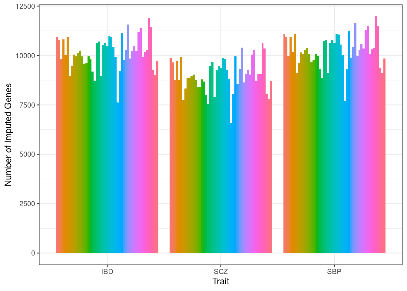
####################

#minimum number of genes
df_plot[which.min(df_plot$n_genes),]
n_genes weight trait
79 6591 Kidney Cortex SCZ#maximum number of genes
df_plot[which.max(df_plot$n_genes),] n_genes weight trait
143 11985 Testis SBP####################
df_plot <- df_plot[rev(1:nrow(df_plot)),]
pdf(file = "output/ALL_number_imputed_genes.pdf", width = 7, height = 10)
par(mar=c(4.1, 9.6, 0.6, 1.6))
barplot(df_plot$n_genes, names.arg=df_plot$weight, las=2, xlab="Number of Imputed Genes", main="",
cex.lab=0.8,
cex.axis=0.8,
cex.names=0.3,
space=c(c(0, rep(0,48)), rep(c(3, rep(0,48)), 2)),
col=rep(c("darkblue", "grey50"),3),
axis.lty=1,
horiz=T,
las=1,
xlim=c(0,12000))
grid(nx = NULL,
ny = NA,
lty = 2, col = "grey", lwd = 1)
dev.off()png
2 ####################
#average over tissues
df_plot <- aggregate(n_genes~weight, df_plot, mean)
pdf(file = "output/ALL_number_imputed_genes_mean.pdf", width = 7, height = 8)
par(mar=c(4.1, 9.6, 0.6, 1.6))
barplot(df_plot$n_genes, names.arg=df_plot$weight, las=2, xlab="Number of Imputed Genes", main="",
cex.lab=0.8,
cex.axis=0.8,
cex.names=0.6,
col=c("darkblue", "grey50"),
axis.lty=1,
horiz=T,
las=1,
xlim=c(0,12000))
grid(nx = NULL,
ny = NA,
lty = 2, col = "grey", lwd = 1)
dev.off()png
2 Number of genes in PredictDB weights
weight_dir <- "/project2/mstephens/wcrouse/predictdb_nolnc/"
weight_files <- list.files(weight_dir)
weight_files <- weight_files[grep(".db", weight_files)]

df_plot <- data.frame(weight=as.character(), n_genes=as.numeric())

for (i in 1:length(weight_files)){
  weight_file <- weight_files[i]

  weight <- unlist(strsplit(weight_file, "mashr_"))[2]
  weight <- unlist(strsplit(weight, "_nolnc.db"))
  weight <- paste(unlist(strsplit(weight, "_")), collapse=" ")

  sqlite <- RSQLite::dbDriver("SQLite")
  db = RSQLite::dbConnect(sqlite, paste0(weight_dir, weight_file))
  query <- function(...) RSQLite::dbGetQuery(db, ...)
  gene_info <- query("select gene, genename, gene_type from extra")
  RSQLite::dbDisconnect(db)

  df_plot_weight <- data.frame(weight=as.character(weight), n_genes=as.numeric(nrow(gene_info)))

  if (i==1){
    df_plot <- df_plot_weight
  } else {
    df_plot <- rbind(df_plot, df_plot_weight)
  }
}

p <- ggplot(df_plot, aes(y=n_genes, x=reorder(weight, dplyr::desc(weight)))) + geom_bar(position="dodge", stat="identity") + xlab("Tissue") + ylab("Number of Protein-Coding Genes")
p <- p + theme_bw() + ylim(0,15100)
p <- p + coord_flip()

p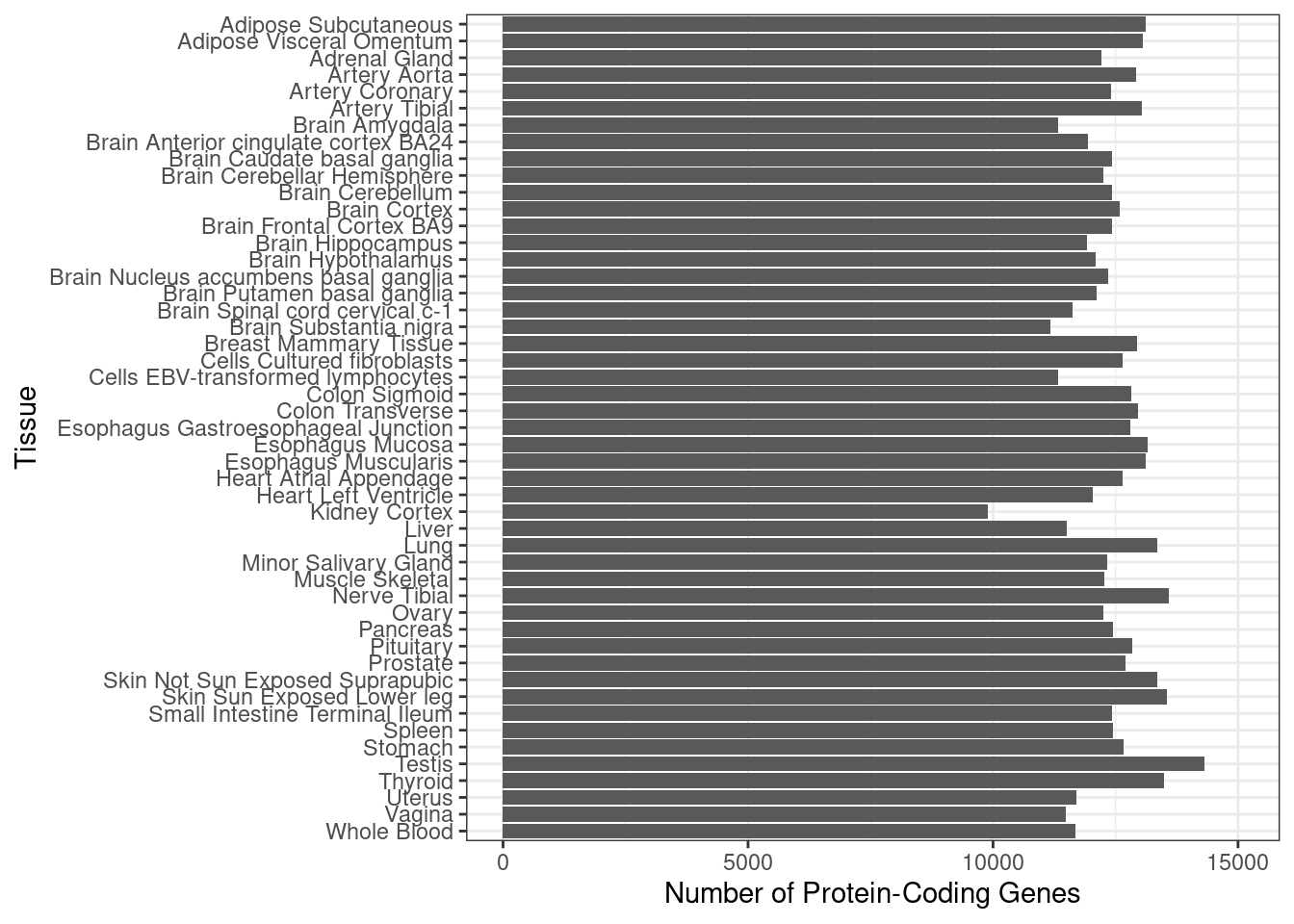
####################

#minimum number of genes
df_plot[which.min(df_plot$n_genes),]
weight n_genes
30 Kidney Cortex 9898#maximum number of genes
df_plot[which.max(df_plot$n_genes),] weight n_genes
45 Testis 14324Estimated parameters for each trait and weight
Prior inclusion
#prior inclusion

for (i in 1:length(df_all)){
  prior <- sapply(df_all[[i]], function(x){x$prior})
  prior <- prior[1,]
  weight <- names(prior)
  weight <- sapply(weight, function(x){paste(unlist(strsplit(x, "_")), collapse=" ")})
  df_plot_trait <- data.frame(prior=prior, weight=weight, trait=trait_names$trait_abbr[i])
  rownames(df_plot_trait) <- NULL

  if (i==1){
    df_plot <- df_plot_trait
  } else {
    df_plot <- rbind(df_plot, df_plot_trait)
  }
}

p <- ggplot(df_plot, aes(x=trait, y=prior)) + geom_boxplot(fill='#A4A4A4', color="black", outlier.shape=NA) + expand_limits(y=0)
p <- p + geom_jitter(shape=16, position=position_jitter(0.2))
p <- p + theme_bw()
p <- p + xlab("Trait") + ylab("Prior Inclusion Probability")

p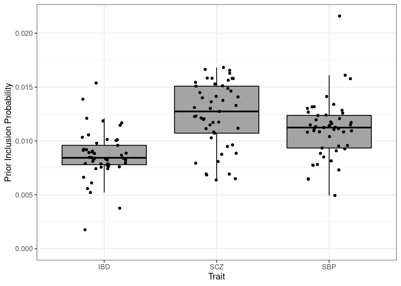
#minimum prior inclusion
df_plot[which.min(df_plot$prior),]
prior weight trait
48 0.001760182 Vagina IBD#maximum prior inclusion
df_plot[which.max(df_plot$prior),] prior weight trait
102 0.02159532 Artery Aorta SBP####################
p_pi <- p + ylab(bquote(pi)) + ggtitle("Proportion Causal")Prior variance
#prior variance

for (i in 1:length(df_all)){
  prior_var <- sapply(df_all[[i]], function(x){x$prior_var})
  prior_var <- prior_var[1,]
  weight <- names(prior_var)
  weight <- sapply(weight, function(x){paste(unlist(strsplit(x, "_")), collapse=" ")})
  df_plot_trait <- data.frame(prior_var=prior_var, weight=weight, trait=trait_names$trait_abbr[i])
  rownames(df_plot_trait) <- NULL

  if (i==1){
    df_plot <- df_plot_trait
  } else {
    df_plot <- rbind(df_plot, df_plot_trait)
  }
}

p <- ggplot(df_plot, aes(x=trait, y=prior_var)) + geom_boxplot(fill='#A4A4A4', color="black", outlier.shape=NA) + expand_limits(y=0)
p <- p + geom_jitter(shape=16, position=position_jitter(0.2))
p <- p + theme_bw()
p <- p + xlab("Trait") + ylab("Prior Variance")

p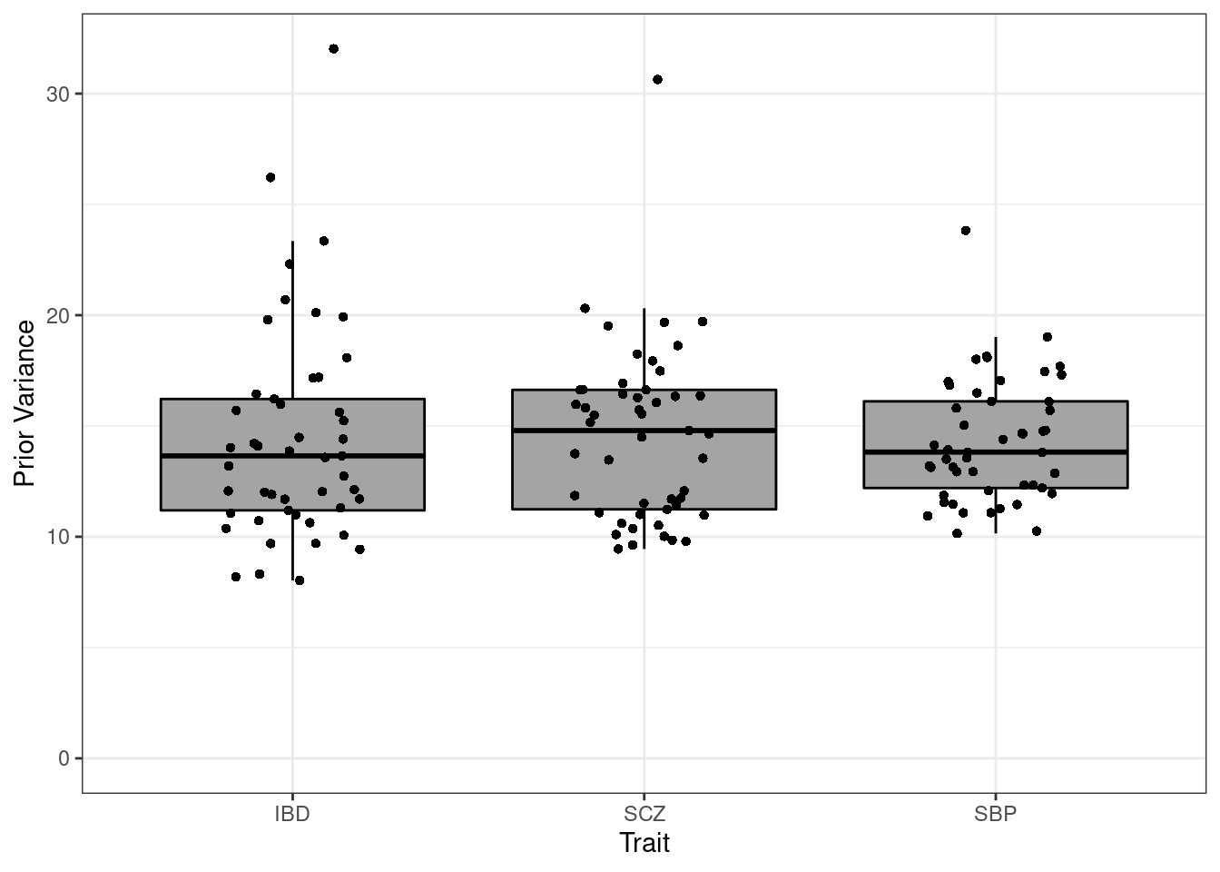
#minimum prior variance
df_plot[which.min(df_plot$prior_var),]
prior_var weight trait
36 8.028828 Ovary IBD#maximum prior variance
df_plot[which.max(df_plot$prior_var),] prior_var weight trait
48 32.02479 Vagina IBD####################
p_sigma2 <- p + ylab(bquote(sigma^2)) + ggtitle("Effect Size")Enrichment
for (i in 1:length(df_all)){
  prior <- sapply(df_all[[i]], function(x){x$prior})
  enrich <- prior[1,]/prior[2,]
  weight <- names(enrich)
  weight <- sapply(weight, function(x){paste(unlist(strsplit(x, "_")), collapse=" ")})
  df_plot_trait <- data.frame(enrich=enrich, weight=weight, trait=trait_names$trait_abbr[i])
  rownames(df_plot_trait) <- NULL

  if (i==1){
    df_plot <- df_plot_trait
  } else {
    df_plot <- rbind(df_plot, df_plot_trait)
  }
}

p <- ggplot(df_plot, aes(x=trait, y=enrich)) + geom_boxplot(fill='#A4A4A4', color="black", outlier.shape=NA) + expand_limits(y=0)
p <- p + geom_jitter(shape=16, position=position_jitter(0.2))
p <- p + theme_bw()
p <- p + xlab("Trait") + ylab("Enrichment")

p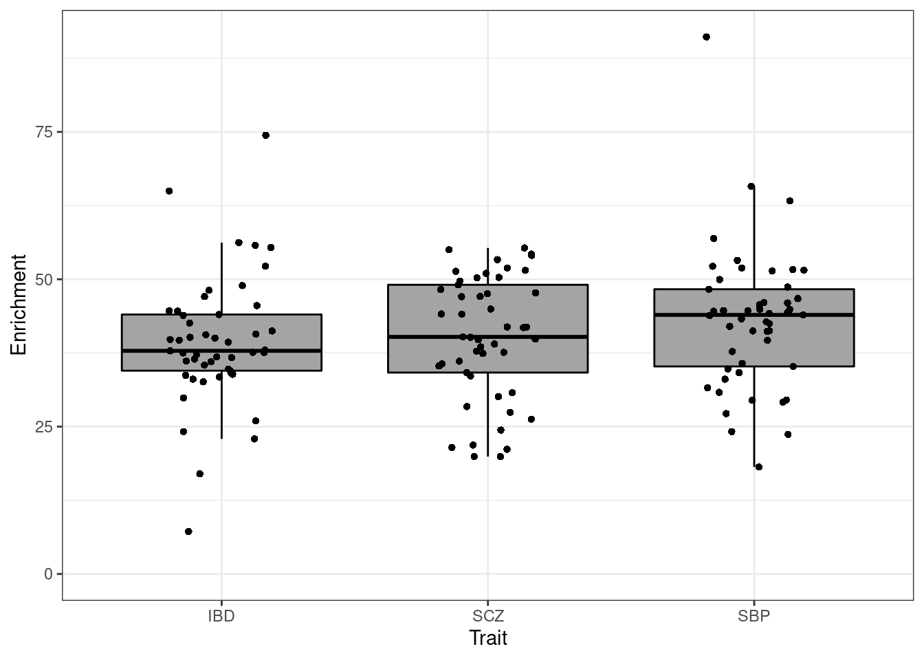
####################

p_enrich <- p + ylab(bquote(pi[G]/pi[S])) + ggtitle("Enrichment")
Proportion of variance explained
#prior variance explained

for (i in 1:length(df_all)){
  pve <- sapply(df_all[[i]], function(x){x$pve})
  pve <- pve[1,]
  weight <- names(pve)
  weight <- sapply(weight, function(x){paste(unlist(strsplit(x, "_")), collapse=" ")})
  df_plot_trait <- data.frame(pve=pve, weight=weight, trait=trait_names$trait_abbr[i])
  rownames(df_plot_trait) <- NULL

  if (i==1){
    df_plot <- df_plot_trait
  } else {
    df_plot <- rbind(df_plot, df_plot_trait)
  }
}

p <- ggplot(df_plot, aes(x=trait, y=pve)) + geom_boxplot(fill='#A4A4A4', color="black", outlier.shape=NA) + expand_limits(y=0)
p <- p + geom_jitter(shape=16, position=position_jitter(0.2))
p <- p + theme_bw()
p <- p + xlab("Trait") + ylab("Proportion of Variance Explained")

p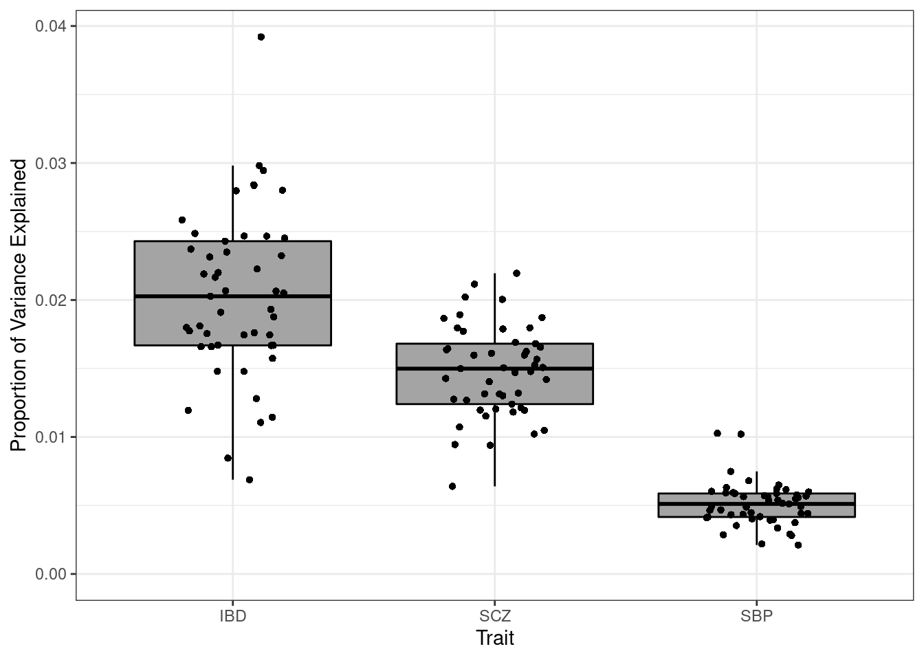
#minimum PVE
df_plot[which.min(df_plot$pve),]
pve weight trait
140 0.002115861 Small Intestine Terminal Ileum SBP#maximum PVE
df_plot[which.max(df_plot$pve),] pve weight trait
49 0.03920475 Whole Blood IBD####################
p_pve <- p + ylab(bquote(h^2[G])) + ggtitle("PVE")Mediated heritability
#mediated heritability

for (i in 1:length(df_all)){
  h2_med <- sapply(df_all[[i]], function(x){x$pve})
  h2_med <- apply(h2_med, 2, function(x){x[1]/(sum(x))})
  weight <- names(h2_med)
  weight <- sapply(weight, function(x){paste(unlist(strsplit(x, "_")), collapse=" ")})
  df_plot_trait <- data.frame(h2_med=h2_med, weight=weight, trait=trait_names$trait_abbr[i])
  rownames(df_plot_trait) <- NULL

  if (i==1){
    df_plot <- df_plot_trait
  } else {
    df_plot <- rbind(df_plot, df_plot_trait)
  }
}

p <- ggplot(df_plot, aes(x=trait, y=h2_med)) + geom_boxplot(fill='#A4A4A4', color="black", outlier.shape=NA) + expand_limits(y=0)
p <- p + geom_jitter(shape=16, position=position_jitter(0.2))
p <- p + theme_bw()
p <- p + xlab("Trait") + ylab("Proportion of Mediated Heritability")

p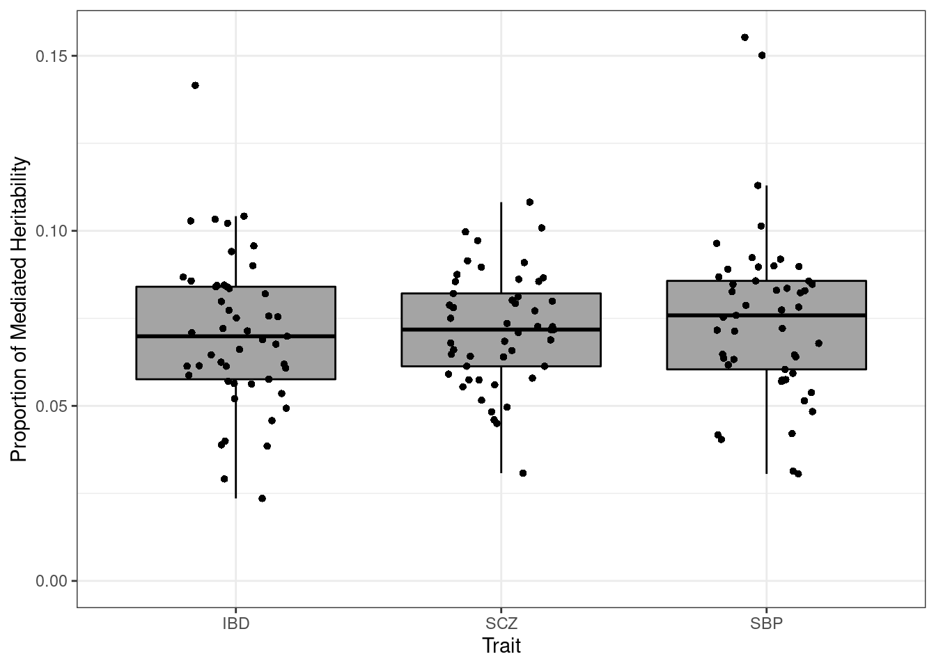
| Version | Author | Date |
|---|---|---|
| 2af4567 | wesleycrouse | 2022-09-02 |
####################
#mediated heritability - top tissues only

n_top_tissues <- 5


for (i in 1:length(df_all)){
  h2_med <- sapply(df_all[[i]], function(x){x$pve})
  h2_med <- apply(h2_med, 2, function(x){x[1]/(sum(x))})

  h2_med <- (-sort(-h2_med))[1:n_top_tissues]

  weight <- names(h2_med)
  weight <- sapply(weight, function(x){paste(unlist(strsplit(x, "_")), collapse=" ")})
  df_plot_trait <- data.frame(h2_med=h2_med, weight=weight, trait=trait_names$trait_abbr[i])
  rownames(df_plot_trait) <- NULL

  if (i==1){
    df_plot <- df_plot_trait
  } else {
    df_plot <- rbind(df_plot, df_plot_trait)
  }
}

p <- ggplot(df_plot, aes(fill=weight, y=h2_med, x=trait)) + geom_bar(position="dodge", stat="identity") + xlab("Trait") + ylab("Proportion of Mediated Heritability")
p <- p + theme_bw()

p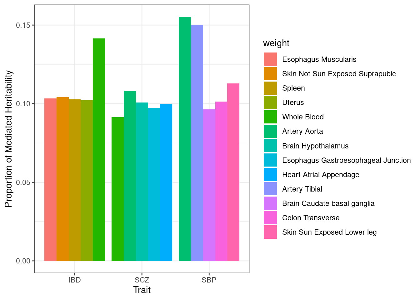
| Version | Author | Date |
|---|---|---|
| 2af4567 | wesleycrouse | 2022-09-02 |
####################
#mediated heritability - top tissues only

n_top_tissues <- 2


for (i in 1:length(df_all)){
  h2_med <- sapply(df_all[[i]], function(x){x$pve})
  h2_med <- apply(h2_med, 2, function(x){x[1]/(sum(x))})

  h2_med <- (-sort(-h2_med))[1:n_top_tissues]

  weight <- names(h2_med)
  weight <- sapply(weight, function(x){paste(unlist(strsplit(x, "_")), collapse=" ")})
  df_plot_trait <- data.frame(h2_med=h2_med, weight=weight, trait=trait_names$trait_abbr[i])
  rownames(df_plot_trait) <- NULL

  if (i==1){
    df_plot <- df_plot_trait
  } else {
    df_plot <- rbind(df_plot, df_plot_trait)
  }
}

p <- ggplot(df_plot, aes(fill=weight, y=h2_med, x=trait)) + geom_bar(position="dodge", stat="identity") + xlab("Trait") + ylab("Proportion of Mediated Heritability")
p <- p + theme_bw()

p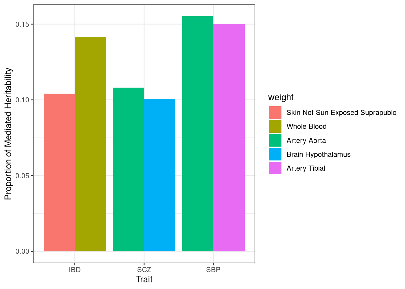
| Version | Author | Date |
|---|---|---|
| 2af4567 | wesleycrouse | 2022-09-02 |
####################

#maximum mediated heritability by trait
aggregate(h2_med ~ trait, data = df_plot, max)
trait h2_med
1 IBD 0.1415441
2 SCZ 0.1081910
3 SBP 0.1552622Plot of all estimated parameters for each trait and weight
library(cowplot)

title_size <- 12

p_pi <- p_pi + theme(plot.title=element_text(size=title_size))
p_sigma2 <- p_sigma2 + theme(plot.title=element_text(size=title_size))
p_enrich <- p_enrich + theme(plot.title=element_text(size=title_size))
p_pve <- p_pve + theme(plot.title=element_text(size=title_size))

pdf(file = "output/ALL_parameters.pdf", width = 6, height = 4)

plot_grid(p_pi, p_sigma2, p_enrich, p_pve)

dev.off()
png
2 Table of all estimated parameters for each trait and weight
for (i in 1:length(df_all)){
  prior <- sapply(df_all[[i]], function(x){x$prior})
  rownames(prior) <- c("prior_g", "prior_s")

  enrich <- prior[1,]/prior[2,]

  prior_var <- sapply(df_all[[i]], function(x){x$prior_var})
  rownames(prior_var) <- c("prior_var_g", "prior_var_s")

  pve <- sapply(df_all[[i]], function(x){x$pve})
  rownames(pve) <- c("pve_g", "pve_s")

  h2 <- colSums(pve)

  prop_h2_g <- apply(pve, 2, function(x){x[1]/sum(x)})

  weight <- colnames(prior)
  trait <- trait_names$trait_abbr[i]

  parameter_table_current <- as.data.frame(t(rbind(prior, prior_var, enrich, pve, h2, prop_h2_g)))

  parameter_table_current <- cbind(trait, weight, parameter_table_current)
  rownames(parameter_table_current) <- NULL

  if (i==1){
    parameter_table <- parameter_table_current
  } else {
    parameter_table <- rbind(parameter_table, parameter_table_current)
  }
}

write.csv(parameter_table, file="output/ALL_parameters.csv" ,row.names=F)
Number of genes in top tissue groups for each trait
weight_groups <- as.data.frame(matrix(c("Adipose_Subcutaneous", "Adipose",
                                        "Adipose_Visceral_Omentum", "Adipose",
                                        "Adrenal_Gland", "Endocrine",
                                        "Artery_Aorta", "Cardiovascular",
                                        "Artery_Coronary", "Cardiovascular",
                                        "Artery_Tibial", "Cardiovascular",
                                        "Brain_Amygdala", "CNS",
                                        "Brain_Anterior_cingulate_cortex_BA24", "CNS",
                                        "Brain_Caudate_basal_ganglia", "CNS",
                                        "Brain_Cerebellar_Hemisphere", "CNS",
                                        "Brain_Cerebellum", "CNS",
                                        "Brain_Cortex", "CNS",
                                        "Brain_Frontal_Cortex_BA9", "CNS",
                                        "Brain_Hippocampus", "CNS",
                                        "Brain_Hypothalamus", "CNS",
                                        "Brain_Nucleus_accumbens_basal_ganglia", "CNS",
                                        "Brain_Putamen_basal_ganglia", "CNS",
                                        "Brain_Spinal_cord_cervical_c-1", "CNS",
                                        "Brain_Substantia_nigra", "CNS",
                                        "Breast_Mammary_Tissue", "None",
                                        "Cells_Cultured_fibroblasts", "Skin",
                                        "Cells_EBV-transformed_lymphocytes", "Blood or Immune",
                                        "Colon_Sigmoid", "Digestive",
                                        "Colon_Transverse", "Digestive",
                                        "Esophagus_Gastroesophageal_Junction", "Digestive",
                                        "Esophagus_Mucosa", "Digestive",
                                        "Esophagus_Muscularis", "Digestive",
                                        "Heart_Atrial_Appendage", "Cardiovascular",
                                        "Heart_Left_Ventricle", "Cardiovascular",
                                        "Kidney_Cortex", "None",
                                        "Liver", "None",
                                        "Lung", "None",
                                        "Minor_Salivary_Gland", "None",
                                        "Muscle_Skeletal", "None",
                                        "Nerve_Tibial", "None",
                                        "Ovary", "None",
                                        "Pancreas", "None",
                                        "Pituitary", "Endocrine",
                                        "Prostate", "None",
                                        "Skin_Not_Sun_Exposed_Suprapubic", "Skin",
                                        "Skin_Sun_Exposed_Lower_leg", "Skin",
                                        "Small_Intestine_Terminal_Ileum", "Digestive",
                                        "Spleen", "Blood or Immune",
                                        "Stomach", "Digestive",
                                        "Testis", "Endocrine",
                                        "Thyroid", "Endocrine",
                                        "Uterus", "None",
                                        "Vagina", "None",
                                        "Whole_Blood", "Blood or Immune"),
                                      nrow=49, ncol=2, byrow=T), stringsAsFactors=F)
colnames(weight_groups) <- c("weight", "group")
n_top_tissue_groups <- 2
for (i in 1:length(df_all)){
trait <- trait_names$trait_abbr[trait_names$trait_id==names(df_all)[i]]
ctwas_genes_by_group <- list()
ctwas_genes_by_tissue <- sapply(df_all[[i]], function(x){x$ctwas})
for (j in 1:length(ctwas_genes_by_tissue)){
weight <- names(ctwas_genes_by_tissue)[j]
group <- weight_groups$group[weight_groups$weight==weight]
ctwas_genes_by_group[[group]] <- c(ctwas_genes_by_group[[group]], ctwas_genes_by_tissue[j])
}
ctwas_genes_by_group$None <- NULL
top_groups <- rev(sort(sapply(ctwas_genes_by_group, function(x){length(unique(unlist(x)))})))[1:n_top_tissue_groups]
df_plot_trait <- data.frame(weight=as.character(names(top_groups)), trait=as.character(trait), n_ctwas=as.numeric(top_groups))
rownames(df_plot_trait) <- NULL
#df_plot_trait <- rbind(df_plot_trait, data.frame(weight="",trait="",n_ctwas=0))
if (i==1){
df_plot <- df_plot_trait
} else {
df_plot <- rbind(df_plot, df_plot_trait)
}
}
ggplot(df_plot, aes(fill=weight, y=n_ctwas, x=trait)) + geom_bar(position="dodge", stat="identity") + xlab("Trait") + ylab("Number of cTWAS Genes")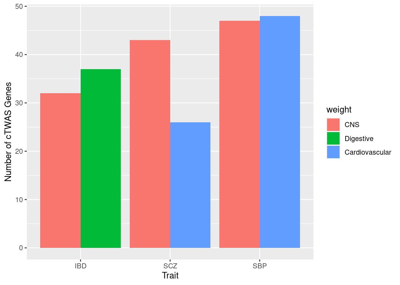
Number of genes in top tissues for each trait
n_top_tissue_groups <- 2

for (i in 1:length(df_all)){
  trait <- trait_names$trait_abbr[trait_names$trait_id==names(df_all)[i]]
  ctwas_genes_by_tissue <- sapply(df_all[[i]], function(x){length(x$ctwas)})
  ctwas_genes_by_tissue <- rev(sort(ctwas_genes_by_tissue))[1:n_top_tissue_groups]

  df_plot_trait <- data.frame(weight=as.character(names(ctwas_genes_by_tissue)), trait=as.character(trait), n_ctwas=as.numeric(ctwas_genes_by_tissue))
  rownames(df_plot_trait) <- NULL

  if (i==1){
    df_plot <- df_plot_trait
  } else {
    df_plot <- rbind(df_plot, df_plot_trait)
  }

}

df_plot$weight <- sapply(as.character(df_plot$weight), function(x){paste(unlist(strsplit(x, "_")), collapse=" ")})

ggplot(df_plot, aes(fill=weight, y=n_ctwas, x=trait)) + geom_bar(position="dodge", stat="identity") + xlab("Trait") + ylab("Number of cTWAS Genes")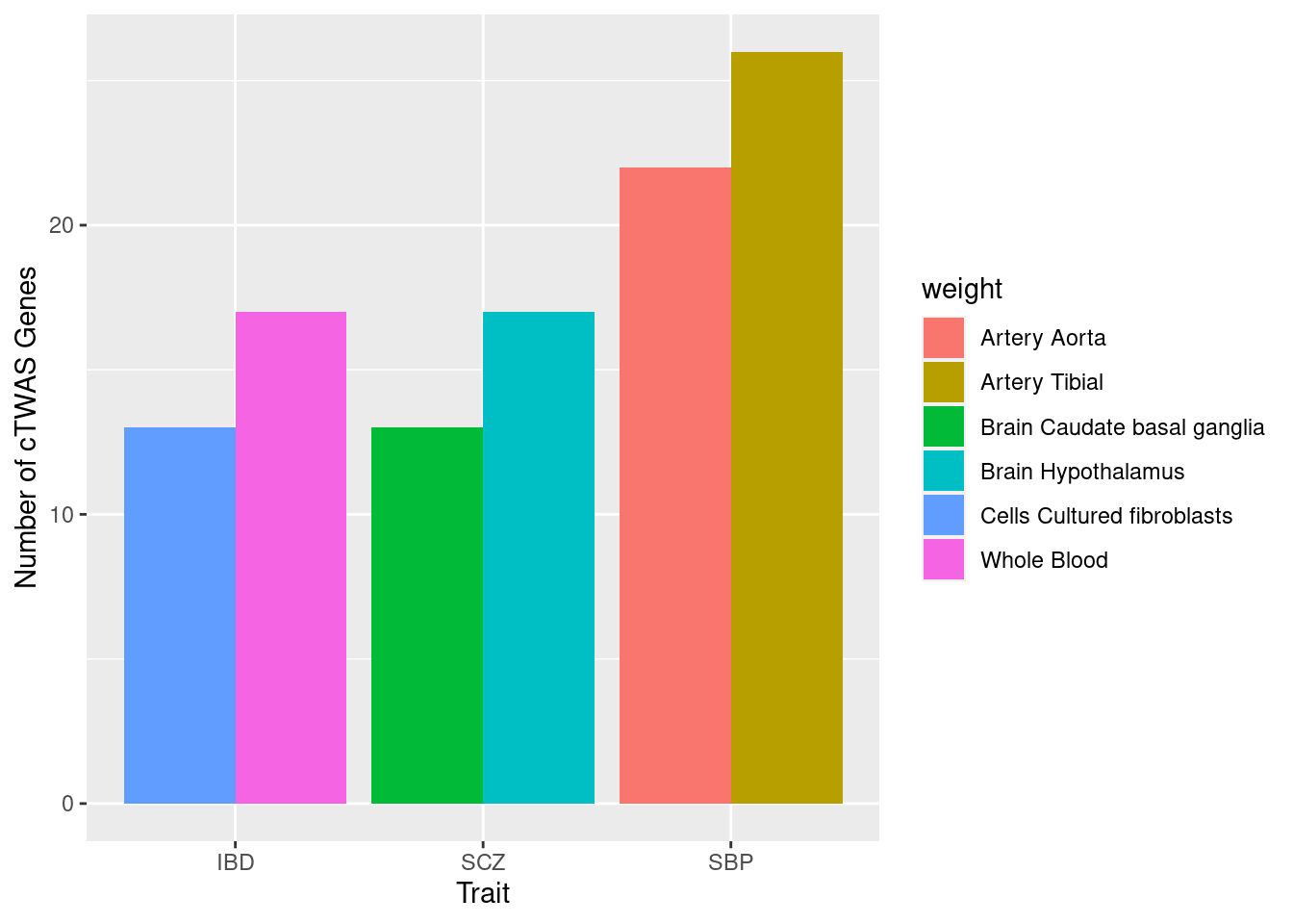
| Version | Author | Date |
|---|---|---|
| 6a57156 | wesleycrouse | 2022-09-14 |
####################

df_plot <-  df_plot[order(as.character(df_plot$trait)),]

pdf(file = "output/ALL_number_ctwas_genes.pdf", width = 2.75, height = 3)

par(mar=c(6.6, 3.6, 1.6, 0.6))

barplot(df_plot$n_ctwas, names.arg=df_plot$weight, las=2, ylab="Number of cTWAS Genes", main="",
        cex.lab=0.7,
        cex.axis=0.7,
        cex.names=0.7,
        space=c(0.4, 0, 0.4, 0, 0.4, 0),
        col=rep(c("grey50", "grey"),3),
        axis.lty=1)

dev.off()
png
2
sessionInfo()R version 3.6.1 (2019-07-05)
Platform: x86_64-pc-linux-gnu (64-bit)
Running under: Scientific Linux 7.4 (Nitrogen)
Matrix products: default
BLAS/LAPACK: /software/openblas-0.2.19-el7-x86_64/lib/libopenblas_haswellp-r0.2.19.so
locale:
[1] LC_CTYPE=en_US.UTF-8 LC_NUMERIC=C
[3] LC_TIME=en_US.UTF-8 LC_COLLATE=en_US.UTF-8
[5] LC_MONETARY=en_US.UTF-8 LC_MESSAGES=en_US.UTF-8
[7] LC_PAPER=en_US.UTF-8 LC_NAME=C
[9] LC_ADDRESS=C LC_TELEPHONE=C
[11] LC_MEASUREMENT=en_US.UTF-8 LC_IDENTIFICATION=C
attached base packages:
[1] stats graphics grDevices utils datasets methods base
other attached packages:
[1] cowplot_1.1.1 ggplot2_3.3.5
loaded via a namespace (and not attached):
[1] Rcpp_1.0.6 pillar_1.7.0 compiler_3.6.1 later_0.8.0
[5] git2r_0.26.1 workflowr_1.6.2 tools_3.6.1 bit_4.0.4
[9] digest_0.6.20 memoise_2.0.0 RSQLite_2.2.7 evaluate_0.14
[13] lifecycle_1.0.1 tibble_3.1.7 gtable_0.3.0 pkgconfig_2.0.3
[17] rlang_1.0.2 DBI_1.1.1 cli_3.3.0 yaml_2.2.0
[21] xfun_0.8 fastmap_1.1.0 withr_2.4.1 stringr_1.4.0
[25] dplyr_1.0.9 knitr_1.23 generics_0.0.2 fs_1.5.2
[29] vctrs_0.4.1 bit64_4.0.5 tidyselect_1.1.2 rprojroot_2.0.2
[33] grid_3.6.1 glue_1.6.2 R6_2.5.0 fansi_0.5.0
[37] rmarkdown_1.13 blob_1.2.1 farver_2.1.0 purrr_0.3.4
[41] magrittr_2.0.3 whisker_0.3-2 scales_1.2.0 promises_1.0.1
[45] ellipsis_0.3.2 htmltools_0.5.2 colorspace_1.4-1 httpuv_1.5.1
[49] labeling_0.3 utf8_1.2.1 stringi_1.4.3 munsell_0.5.0
[53] cachem_1.0.5 crayon_1.4.1