metabolites_h2
wesleycrouse
2021-09-7
Last updated: 2021-09-22
Checks: 7 0
Knit directory: ctwas_applied/
This reproducible R Markdown analysis was created with workflowr (version 1.6.2). The Checks tab describes the reproducibility checks that were applied when the results were created. The Past versions tab lists the development history.
Great! Since the R Markdown file has been committed to the Git repository, you know the exact version of the code that produced these results.
Great job! The global environment was empty. Objects defined in the global environment can affect the analysis in your R Markdown file in unknown ways. For reproduciblity it’s best to always run the code in an empty environment.
The command set.seed(20210726) was run prior to running the code in the R Markdown file. Setting a seed ensures that any results that rely on randomness, e.g. subsampling or permutations, are reproducible.
Great job! Recording the operating system, R version, and package versions is critical for reproducibility.
Nice! There were no cached chunks for this analysis, so you can be confident that you successfully produced the results during this run.
Great job! Using relative paths to the files within your workflowr project makes it easier to run your code on other machines.
Great! You are using Git for version control. Tracking code development and connecting the code version to the results is critical for reproducibility.
The results in this page were generated with repository version 3b55290. See the Past versions tab to see a history of the changes made to the R Markdown and HTML files.
Note that you need to be careful to ensure that all relevant files for the analysis have been committed to Git prior to generating the results (you can use wflow_publish or wflow_git_commit). workflowr only checks the R Markdown file, but you know if there are other scripts or data files that it depends on. Below is the status of the Git repository when the results were generated:
working directory clean
Note that any generated files, e.g. HTML, png, CSS, etc., are not included in this status report because it is ok for generated content to have uncommitted changes.
These are the previous versions of the repository in which changes were made to the R Markdown (analysis/metabolites_h2.Rmd) and HTML (docs/metabolites_h2.html) files. If you’ve configured a remote Git repository (see ?wflow_git_remote), click on the hyperlinks in the table below to view the files as they were in that past version.
| File | Version | Author | Date | Message |
|---|---|---|---|---|
| Rmd | 3b55290 | wesleycrouse | 2021-09-22 | h2 plot |
| Rmd | ffe73a3 | wesleycrouse | 2021-09-22 | updated h2 report |
| html | 286be0b | wesleycrouse | 2021-09-20 | no label |
| html | f44b453 | wesleycrouse | 2021-09-20 | labels |
| html | a0a439f | wesleycrouse | 2021-09-20 | final plots |
| html | a8310a3 | wesleycrouse | 2021-09-20 | plot tinkering |
| html | 4891a34 | wesleycrouse | 2021-09-20 | tinkering |
| html | 5098b56 | wesleycrouse | 2021-09-20 | more plot changes |
| html | 4bf6fa7 | wesleycrouse | 2021-09-20 | plot adjustments |
| html | 43712b3 | wesleycrouse | 2021-09-20 | h2 update |
| Rmd | 0b82945 | wesleycrouse | 2021-09-20 | edits to h2 report |
| html | e5441f9 | wesleycrouse | 2021-09-16 | ppv by pip |
| html | b2ff1b3 | wesleycrouse | 2021-09-16 | h2 plots |
| Rmd | 2eb9138 | wesleycrouse | 2021-09-16 | h2 plots |
| html | 7e22565 | wesleycrouse | 2021-09-13 | updating reports |
| html | cbf7408 | wesleycrouse | 2021-09-08 | adding enrichment to reports |
| html | 4970e3e | wesleycrouse | 2021-09-08 | updating reports |
| html | 0a4f672 | wesleycrouse | 2021-09-07 | running workflowr |
| Rmd | c644749 | wesleycrouse | 2021-09-07 | fixing margins |
| html | cc77344 | wesleycrouse | 2021-09-07 | updating h2 report |
| Rmd | 60eecdf | wesleycrouse | 2021-09-07 | fixing table width |
| html | eb9aa95 | wesleycrouse | 2021-09-07 | h2 report |
| Rmd | 020e3fa | wesleycrouse | 2021-09-07 | fixing workflowr warnings |
| html | 020e3fa | wesleycrouse | 2021-09-07 | fixing workflowr warnings |
| Rmd | ef18712 | wesleycrouse | 2021-09-07 | fixing absolute file path |
| html | ef18712 | wesleycrouse | 2021-09-07 | fixing absolute file path |
| html | 627a4e1 | wesleycrouse | 2021-09-07 | adding heritability |
| Rmd | dfd2b5f | wesleycrouse | 2021-09-07 | regenerating reports |
Heritability of UK Biobank metabolites
Estimates of heritability from ctwas, compared with estimates of heritability from Neale Lab Heritability Browser using LD Score Regression.
#load h2 from Neale Lab
h2_neale <- read.csv("/project2/mstephens/wcrouse/UKB_analysis_old/ukbb_neale_v3_metabolites_h2.csv", head=T)
rownames(h2_neale) <- h2_neale$ID
#compute h2 from ctwas
traits <- read.csv("/project2/mstephens/wcrouse/UKB_analysis/ukbb_neale_v3_metabolites.csv", head=F)
colnames(traits) <- c("trait_name", "neale_id", "ieu_id")
weights <- c("Liver", "Whole_Blood")
# h2_table <- matrix(NA,nrow(traits),2*length(weights))
#
# for (weight_index in 1:length(weights)){
# weight <- as.character(weights[weight_index])
#
# print(weight)
#
# for (trait_index in 1:nrow(traits)){
# analysis_id <- paste0(traits$ieu[trait_index], "_", weights[weight_index])
# trait_id <- as.character(traits$ieu[trait_index])
#
# print(trait_id)
#
# results_dir <- paste0("/project2/mstephens/wcrouse/UKB_analysis_old/", trait_id, "/", weight)
#
# if (file.exists(paste0("/project2/mstephens/wcrouse/UKB_analysis_old/", trait_id, "/", weight, "/", trait_id, "_ctwas.susieIrss.txt"))){
# #load thin argument
# source("/project2/mstephens/wcrouse/UKB_analysis_old/ctwas_config.R")
#
# #load sample size
# vcf_file <- paste0("/project2/compbio/gwas_summary_statistics/ukbb_neale_v3/", trait_id, ".vcf")
# sample_size <- unlist(VariantAnnotation::readGeno(vcf_file, "SS"))
# sample_size <- as.numeric(names(which.max(table(sample_size))))
#
# #get number of SNPs from s1 results; adjust for thin
# ctwas_res_s1 <- data.table::fread(paste0(results_dir, "/", analysis_id, "_ctwas.s1.susieIrss.txt"))
# n_snps <- sum(ctwas_res_s1$type=="SNP")/thin
# n_genes <- sum(ctwas_res_s1$type == "gene")
# rm(ctwas_res_s1)
#
# #load results from parameter estimation
# load(paste0(results_dir, "/", analysis_id, "_ctwas.s2.susieIrssres.Rd"))
#
# #estimated group prior
# estimated_group_prior <- group_prior_rec[,ncol(group_prior_rec)]
# names(estimated_group_prior) <- c("gene", "snp")
# estimated_group_prior["snp"] <- estimated_group_prior["snp"]*thin #adjust parameter to account for thin argument
#
# #estimated group prior variance
# estimated_group_prior_var <- group_prior_var_rec[,ncol(group_prior_var_rec)]
# names(estimated_group_prior_var) <- c("gene", "snp")
#
# #store group size
# group_size <- c(n_genes, n_snps)
#
# #estimated group PVE
# estimated_group_pve <- estimated_group_prior_var*estimated_group_prior*group_size/sample_size #check PVE calculation
# names(estimated_group_pve) <- c("gene", "snp")
#
# #store PVE
# h2_table[trait_index,(2*weight_index-1):(2*weight_index)] <- estimated_group_pve
# }
# }
# }
#
# save(h2_table, file="output/h2_table.RData")
load("output/h2_table.RData")
h2_table <- data.frame(h2_table)
colnames(h2_table) <- paste(rep(weights,each=2), rep(c("Gene", "SNP"), 2), sep="_")
rownames(h2_table) <- as.character(traits$ieu_id)
h2_neale <- h2_neale[rownames(h2_table),]
for (weight in weights){
print(weight)
h2_mesc <- data.table::fread(paste0("/project2/xinhe/shared_data/cTWAS/MESC/h2med/h2med_", weight, "_result.txt"))
df <- data.frame(trait=h2_neale$Trait ,ID=h2_neale$ID ,ldsc=h2_neale$Neale_h2, ctwas_SNP=h2_table[,paste0(weight, "_SNP")], ctwas_gene=h2_table[,paste0(weight, "_Gene")])
df$ctwas_total <- df$ctwas_SNP + df$ctwas_gene
df$ctwas_bygene <- df$ctwas_gene/df$ctwas_total
df$h2med_prop <- h2_mesc$h2med_prop
df$ldsc <- round(df$ldsc,3)
df$ctwas_SNP <- round(df$ctwas_SNP,3)
df$ctwas_gene <- round(df$ctwas_gene,3)
df$ctwas_total <- round(df$ctwas_total,3)
print(df[,c("trait", "ldsc", "ctwas_SNP", "ctwas_gene", "ctwas_bygene")])
par(mfrow=c(1,2), oma=c(0,0,0,0))
plot(df$ldsc, df$ctwas_total, xlab="SNP h2 using LDSR", ylab="Total PVE (Gene + SNP) using cTWAS", xlim=c(0,1), ylim=c(0,1), pty=2, pch=21, bg="blue", cex=1.5)
abline(a=0, b=1, lty=2)
hist(df$ctwas_bygene, main="", xlab="(Gene PVE) / (Total PVE)", col="darkgrey", xlim=c(0,1))
mtext(paste0("PVE by SNPs and ", weight, " Genes using cTWAS"), line=-2.5, side=3, outer=TRUE, cex=1.5)
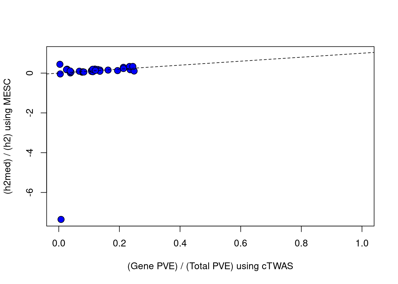
#plot vs MESC
par(mfrow=c(1,1))
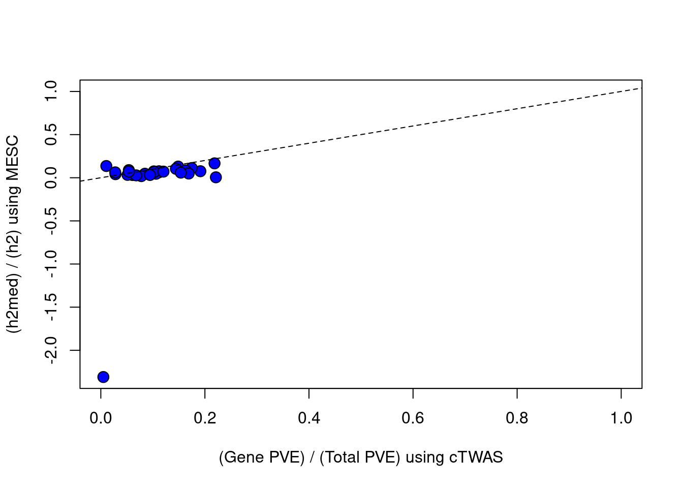
plot(df$ctwas_bygene, df$h2med_prop, ylab="(h2med) / (h2) using MESC", xlab="(Gene PVE) / (Total PVE) using cTWAS", ylim=c(min(df$h2med_prop),1), xlim=c(0,1), pty=2, pch=21, bg="blue", cex=1.5)
abline(a=0, b=1, lty=2)
#correlation between cTWAS and MESC
cor(df$ctwas_bygene, df$h2med_prop, use="complete.obs")
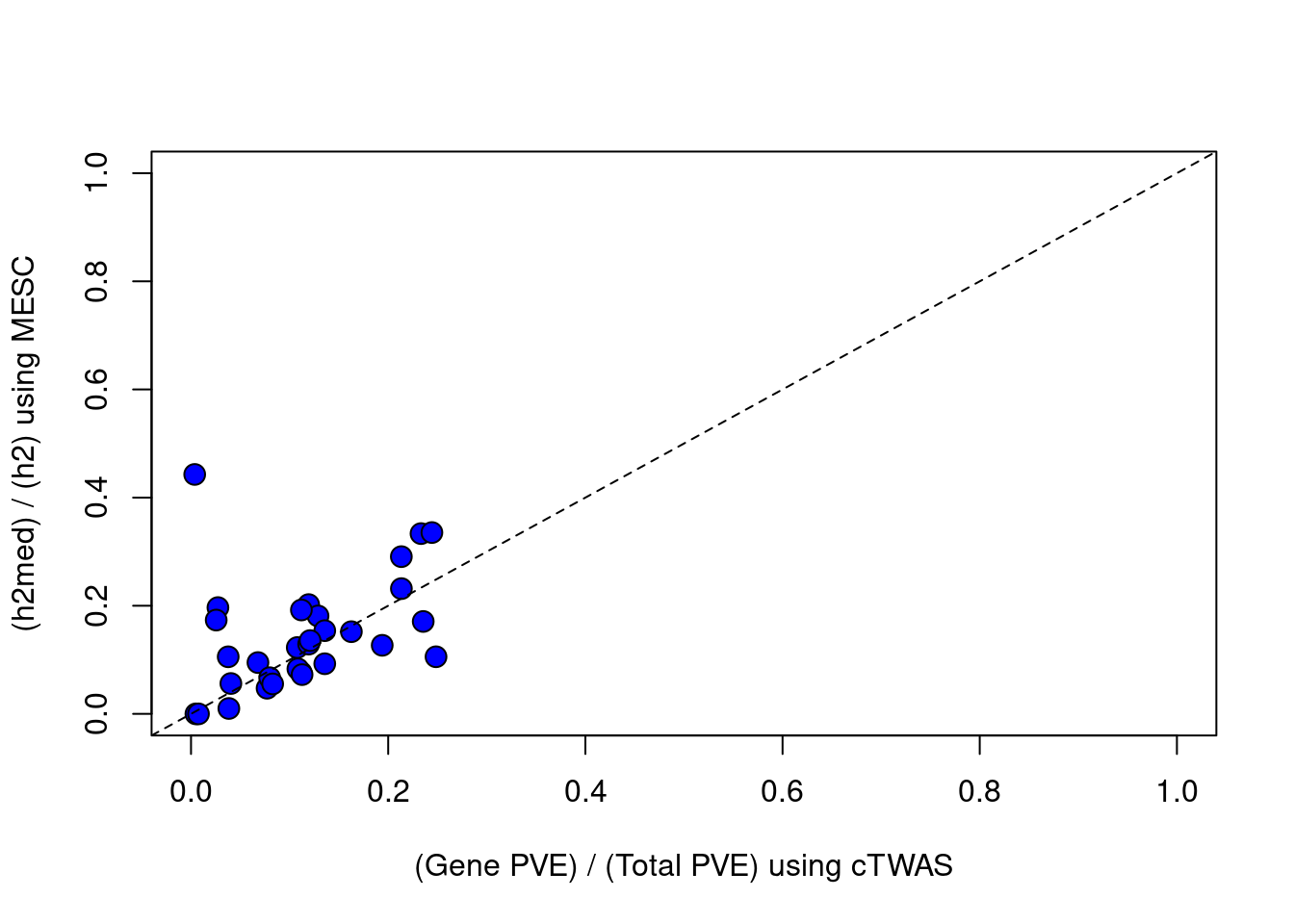
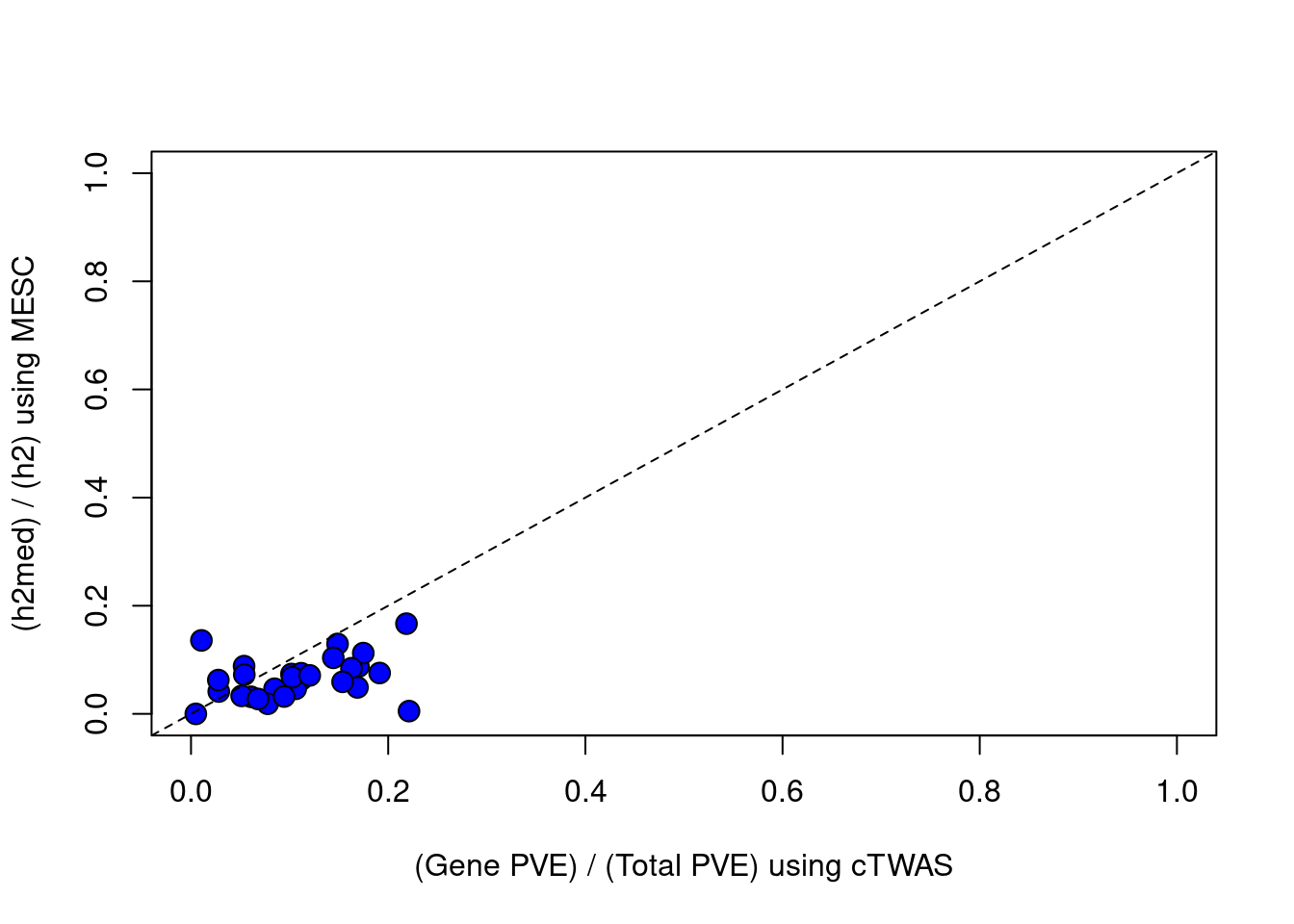
#plot vs MESC, set MESC estimates < 0 to = 0
df$h2med_prop[df$h2med_prop<0] = 0
plot(df$ctwas_bygene, df$h2med_prop, ylab="(h2med) / (h2) using MESC", xlab="(Gene PVE) / (Total PVE) using cTWAS", ylim=c(0,1), xlim=c(0,1), pty=2, pch=21, bg="blue", cex=1.5)
abline(a=0, b=1, lty=2)
#correlation between cTWAS and MESC
cor(df$ctwas_bygene, df$h2med_prop, use="complete.obs")
}[1] "Liver"
trait ldsc ctwas_SNP ctwas_gene
1 Microalbumin in urine 0.043 0.021 0.001
2 Albumin (quantile) 0.145 0.066 0.020
3 Alkaline phosphatase (quantile) 0.309 0.126 0.017
4 Alanine aminotransferase (quantile) 0.132 0.059 0.012
5 Apoliprotein A (quantile) 0.285 0.103 0.015
6 Apoliprotein B (quantile) 0.092 0.047 0.013
7 Aspartate aminotransferase (quantile) 0.143 0.065 0.008
8 Direct bilirubin (quantile) 0.438 0.321 0.009
9 Urea (quantile) 0.119 0.066 0.006
10 Calcium (quantile) 0.135 0.068 0.023
11 Cholesterol (quantile) 0.112 0.052 0.016
12 Creatinine (quantile) 0.211 0.108 0.008
13 C-reactive protein (quantile) 0.193 0.076 0.009
14 Cystatin C (quantile) 0.321 0.121 0.005
15 Gamma glutamyltransferase (quantile) 0.228 0.084 0.023
16 Glucose (quantile) 0.089 0.046 0.004
17 Glycated haemoglobin (quantile) 0.196 0.109 0.013
18 HDL cholesterol (quantile) 0.330 0.123 0.017
19 IGF-1 (quantile) 0.253 0.131 0.017
20 LDL direct (quantile) 0.082 0.043 0.014
21 Lipoprotein A (quantile) 0.127 0.344 0.001
22 Oestradiol (quantile) 0.030 0.025 0.000
23 Phosphate (quantile) 0.134 0.069 0.006
24 Rheumatoid factor (quantile) 0.000 0.029 0.000
25 SHBG (quantile) 0.230 0.149 0.019
26 Total bilirubin (quantile) 0.543 0.470 0.012
27 Testosterone (quantile) 0.077 0.045 0.007
28 Total protein (quantile) 0.167 0.078 0.012
29 Triglycerides (quantile) 0.218 0.135 0.019
30 Urate (quantile) 0.214 0.098 0.004
31 Vitamin D (quantile) 0.100 0.039 0.009
ctwas_bygene
1 0.038381677
2 0.235525865
3 0.119324100
4 0.162635523
5 0.128832694
6 0.213319698
7 0.111620083
8 0.027296214
9 0.077144489
10 0.248507546
11 0.233288296
12 0.067890861
13 0.107756155
14 0.040429643
15 0.213379369
16 0.079757954
17 0.108399242
18 0.119331063
19 0.112641790
20 0.244313605
21 0.003733179
22 0.004961406
23 0.082814678
24 0.007551567
25 0.111943193
26 0.025543011
27 0.135648483
28 0.135644968
29 0.120787853
30 0.037708051
31 0.193929529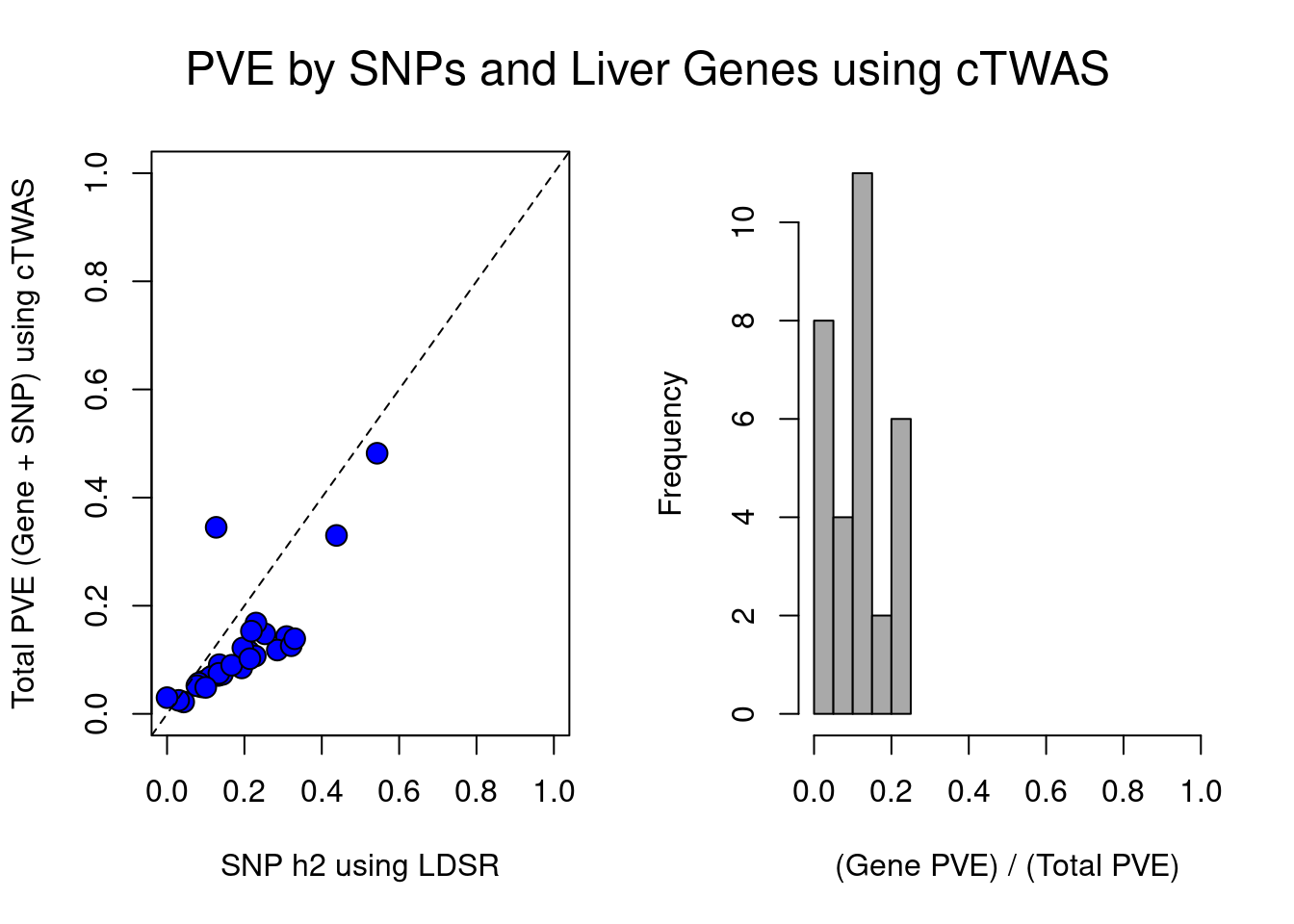
[1] "Whole_Blood"
                                   trait  ldsc ctwas_SNP ctwas_gene
1                  Microalbumin in urine 0.043     0.023      0.002
2                     Albumin (quantile) 0.145     0.070      0.012
3        Alkaline phosphatase (quantile) 0.309     0.114      0.032
4    Alanine aminotransferase (quantile) 0.132     0.057      0.007
5              Apoliprotein A (quantile) 0.285     0.085      0.017
6              Apoliprotein B (quantile) 0.092     0.088      0.021
7  Aspartate aminotransferase (quantile) 0.143     0.064      0.007
8            Direct bilirubin (quantile) 0.438     0.311      0.009
9                        Urea (quantile) 0.119     0.061      0.004
10                    Calcium (quantile) 0.135     0.077      0.010
11                Cholesterol (quantile) 0.112     0.066      0.008
12                 Creatinine (quantile) 0.211     0.108      0.009
13         C-reactive protein (quantile) 0.193     0.072      0.008
14                 Cystatin C (quantile) 0.321     0.108      0.006
15  Gamma glutamyltransferase (quantile) 0.228        NA         NA
16                    Glucose (quantile) 0.089     0.045      0.003
17       Glycated haemoglobin (quantile) 0.196     0.108      0.023
18            HDL cholesterol (quantile) 0.330     0.099      0.019
19                      IGF-1 (quantile) 0.253     0.134      0.014
20                 LDL direct (quantile) 0.082     0.069      0.014
21              Lipoprotein A (quantile) 0.127        NA         NA
22                 Oestradiol (quantile) 0.030     0.023      0.000
23                  Phosphate (quantile) 0.134        NA         NA
24          Rheumatoid factor (quantile) 0.000     0.030      0.000
25                       SHBG (quantile) 0.230     0.153      0.009
26            Total bilirubin (quantile) 0.543     0.455      0.013
27               Testosterone (quantile) 0.077     0.045      0.006
28              Total protein (quantile) 0.167     0.074      0.013
29              Triglycerides (quantile) 0.218     0.123      0.022
30                      Urate (quantile) 0.214     0.094      0.005
31                  Vitamin D (quantile) 0.100     0.037      0.011
   ctwas_bygene
1   0.084719874
2   0.148615724
3   0.218520335
4   0.111751648
5   0.169837692
6   0.191309229
7   0.101887630
8   0.028140381
9   0.060840420
10  0.111707309
11  0.106192787
12  0.077809483
13  0.102581444
14  0.051368901
15           NA
16  0.067999961
17  0.174728537
18  0.162732925
19  0.094449719
20  0.168825813
21           NA
22  0.010556274
23           NA
24  0.004872317
25  0.053826691
26  0.027710232
27  0.120412260
28  0.144313528
29  0.153739016
30  0.054033407
31  0.221119092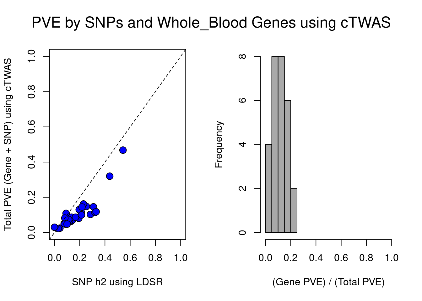
sessionInfo()R version 3.6.1 (2019-07-05)
Platform: x86_64-pc-linux-gnu (64-bit)
Running under: Scientific Linux 7.4 (Nitrogen)
Matrix products: default
BLAS/LAPACK: /software/openblas-0.2.19-el7-x86_64/lib/libopenblas_haswellp-r0.2.19.so
locale:
[1] LC_CTYPE=en_US.UTF-8 LC_NUMERIC=C
[3] LC_TIME=en_US.UTF-8 LC_COLLATE=en_US.UTF-8
[5] LC_MONETARY=en_US.UTF-8 LC_MESSAGES=en_US.UTF-8
[7] LC_PAPER=en_US.UTF-8 LC_NAME=C
[9] LC_ADDRESS=C LC_TELEPHONE=C
[11] LC_MEASUREMENT=en_US.UTF-8 LC_IDENTIFICATION=C
attached base packages:
[1] stats graphics grDevices utils datasets methods base
loaded via a namespace (and not attached):
[1] workflowr_1.6.2 Rcpp_1.0.6 rprojroot_2.0.2
[4] digest_0.6.20 later_0.8.0 R6_2.5.0
[7] git2r_0.26.1 magrittr_2.0.1 evaluate_0.14
[10] stringi_1.4.3 data.table_1.14.0 fs_1.3.1
[13] promises_1.0.1 whisker_0.3-2 rmarkdown_1.13
[16] tools_3.6.1 stringr_1.4.0 glue_1.4.2
[19] httpuv_1.5.1 xfun_0.8 yaml_2.2.0
[22] compiler_3.6.1 htmltools_0.3.6 knitr_1.23